Design of a Parameter-Dependent Optimal Vibration Control of a Non-Linear Vehicle Suspension System

Abstract

This paper is concerned with the design of a parameter-dependent optimal controller for an active vibration attenuation problem of a non-linear vehicle system. A five degree-of-freedom vertical vibration model having an integrated vehicle seat, a non-linear vehicle suspension system, and a seated human body is presented to analyze ride comfort and safety requirements under different types of road disturbances. In the suspension system, the non-linear parts of spring and damper dynamics are considered as scheduling parameters, which are measurable and available for feedback. Then, a parameter-dependent optimal state-feedback controller design that minimizes L₂ gain from disturbance to performance output for a linear parameter-varying (LPV) system is presented with linear matrix inequality (LMI) constraints. Finally, numerical simulations are conducted to demonstrate the effectiveness of the proposed controller.

1. Introduction

Suspension systems are one of the most critical parts of a vehicle. A successfully designed suspension system should be able to provide safety for the passengers and protect the vehicle from damage caused by road irregularities [1]. Dynamic loads in vehicles resulting from road irregularities are recognized as a significant factor in causing fatigue damage. In addition, ground-induced vibrations can contribute to a reduction in the driver’s capability to control the vehicle and cause discomfort [2]. Therefore, a vehicle suspension system has to mitigate vertical vibrations to improve safety and ride comfort performance simultaneously.

Vehicle suspension has been extensively studied for a long time. For all vehicles, passive suspension is designed as a primary suspension system to provide ride comfort, tire deflection, and other dynamic characteristics. A well-designed passive suspension system can mitigate ground-induced vibrations. The problem of the passive vehicle suspension design with an inerter has been taken into account by Hu et al., concerning the multiple performance requirements including ride comfort suspension deflection and tire grip, and the analytical solutions of the designed six-suspension configurations have been derived [3]. Chen et al. have proposed an efficient H₂ optimization method to design passive vehicle suspensions based on a full car model [4]. In the literature, numerous types of semi-active and active suspensions are currently employed and studied, since the capability of passive suspensions is limited due to the absence of on-line control action. Chen et al. have proposed a novel structure for a semi-active suspension with an inerter, which consists of a passive part and semi-active part, to obtain performance benefits in their brief study [5]. The active suspension systems especially have been attracting attention in recent years, and many linear and non-linear control methods for active seat and suspension systems have been proposed [6]. Guclu has designed a fuzzy logic controller for reducing seat vibrations of a non-linear full vehicle model [7]. A seat and suspension system with a driver model has been considered in Gundogdu, and an optimal controller has been designed by the use of a genetic algorithm [8]. Hu et al. have designed a multiplexed model predictive control for active vehicle suspension systems under the consideration of actuator saturation [9]. Gysen et al. have proposed an electromagnetic suspension system to provide additional stability and maneuverability conditions as well as the elimination of road irregularities for vehicle systems [10]. Wang et al. have developed a high-force density tubular permanent motor for an active vehicle suspension system in terms of performance optimization [11]. Onat et al. have applied a linear parameter-varying (LPV) model-based gain-scheduling controller for a full vehicle active suspension system [12]. Fialho and Balos have dealt with the LPV gain-scheduling controller for a road adaptive active suspension system [13]. Among these aforementioned works, it is apparently seen that there are only a few results concerning non-linear suspension control via a parameter-dependent optimal controller to evaluate ride comfort performance in terms of driver body acceleration responses under worst-case road excitations, which is the main motivation factor of this study.

In this paper, the design of a parameter-dependent optimal state-feedback controller is developed to mitigate the ground-induced vertical vibration of a non-linear vehicle system. A proposed controller synthesis is accomplished for the LPV model of non-linear vehicle suspension such that a minimum allowable disturbance attenuation level could be achieved by satisfying a set of LMIs. In the suspension system, the non-linear part of a position-dependent spring and velocity-dependent damping characteristics are assumed as scheduling parameters. In order to reach realistic results, road bumps and very poor random road profiles, are modeled and used as disturbance input. Finally, numerical simulation studies have been presented to illustrate the effectiveness of the proposed approach.

2. Integrated Vehicle Seat and Non-Linear Suspension Model with Driver Body

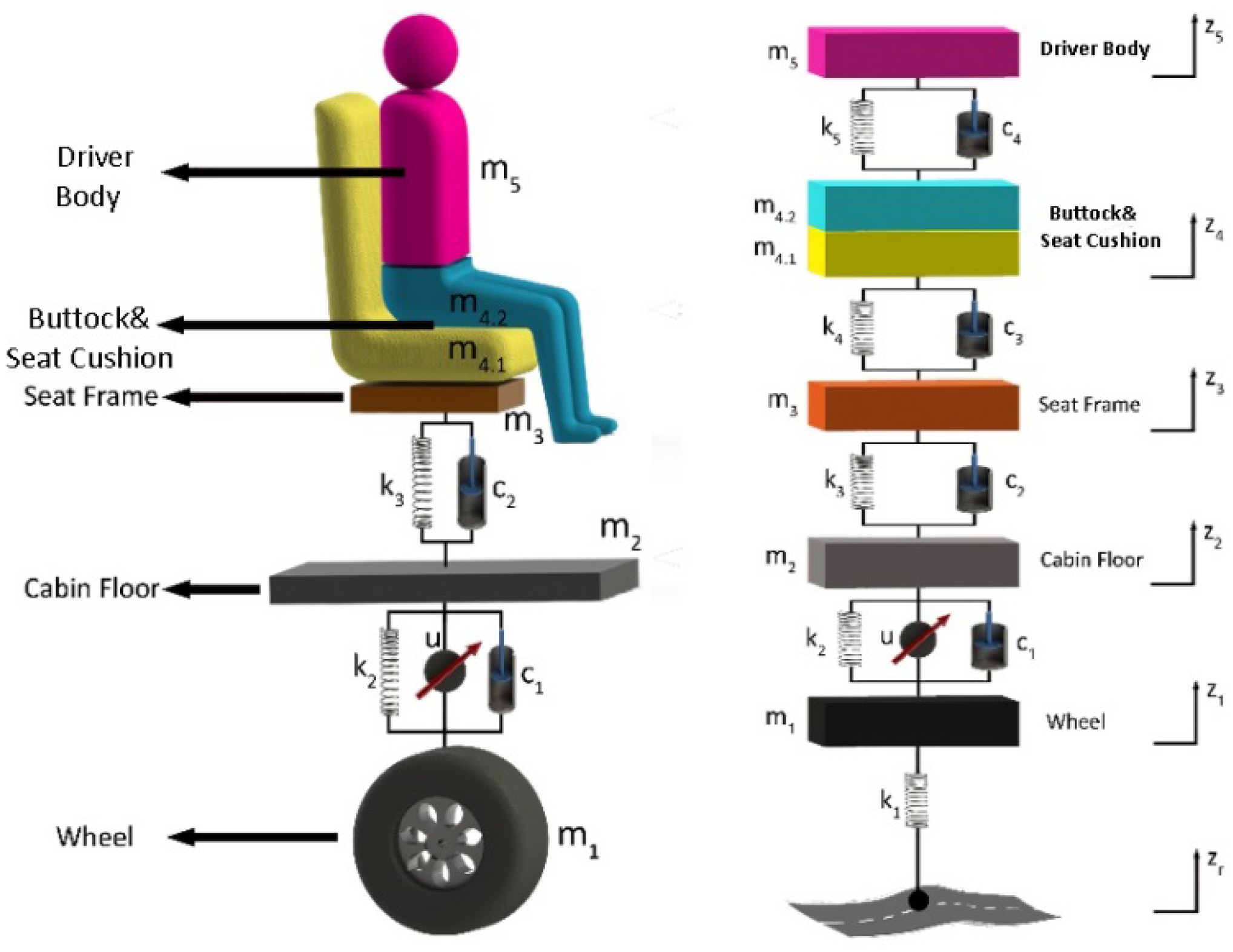
In this study, a five-degree-of-freedom vehicle model, including a quarter car non-linear suspension model, a seat suspension model, and a driver body model, shown in Figure 1, is considered for the parameter-dependent optimal controller design. This integrated model provides a platform to evaluate ride comfort and vehicle safety performance requirements in terms of driver body acceleration, suspension stroke, and tire deflection responses under worst-case random road disturbances and to develop a parameter-dependent optimal control of a non-linear vehicle suspension system. In this figure, m₁ is the unsprung mass, which represents the wheel assembly, m₂ is the quarter car sprung mass, which represents the vehicle cabin floor, m₃ is the mass of the seat frame, m₄₁ and m₄₂ are the masses of human thighs together with buttocks and seated cushion, respectively, and m₅ is the mass of the upper body of a seated human. z₁(t), z₂(t), z₃(t), z₄(t), and z₅(t) are the vertical displacements of the corresponding masses, respectively, and z_r(t) is the road disturbance input. k₁ is the coefficient of tire spring, c₁ and k₂ are the damping and stiffness of the vehicle suspension system, respectively. c₂, c₃ and k₃, k₄ are damping and stiffness of the passive seat suspension system, respectively, and c₄ and k₅ stand for the damping and stiffness of the components inside the human body. In addition, u(t) represents the active control force that is applied to the vehicle suspension. The characteristics of the non-linear spring of the vehicle suspension, which is the mathematical model of the well-known hardening spring behavior, is described as follows:

$$Spring Force=F_s=[k_2+0.1k_2{(z_2(t)-z_1(t))}^2](z_2(t)-z_1(t))$$

(1)

Similar dynamical models with position-dependent stiffness coefficients have been previously reported in the literature [14,15,16]. The quadratic damping feature of the suspension system can be mathematically modeled as:

$$Damper Force=F_d=[c_1+0.41c_1\left|{\dot{z}}_2(t)-{\dot{z}}_1(t)\right|]({\dot{z}}_2(t)-{\dot{z}}_1(t))$$

(2)

where the damping coefficient is non-linear. Additionally, the change of the damping coefficient due to the velocity is discussed in [10,14]. The dynamic vertical motion of equations for the quarter car active suspension, seat suspension, and driver body are given by

$$\begin{array}{l}{m}_1{\ddot{z}}_1(t)+k_1{z}_1(t)-[k_2+0.1k_2{(z_2(t)-z_1(t))}^2](z_2(t)-z_1(t))\\ -[c_1+0.41c_1\left|{\dot{z}}_2(t)-{\dot{z}}_1(t)\right|]({\dot{z}}_2(t)-{\dot{z}}_1(t))=k_1{z}_r(t)+u(t)\end{array}$$

(3)

$$\begin{array}{l}{m}_2{\ddot{z}}_2(t)+[k_2+0.1k_2{(z_2(t)-z_1(t))}^2](z_2(t)-z_1(t))-k_3(z_3(t)-z_2(t))\\ +[c_1+0.41c_1\left|{\dot{z}}_2(t)-{\dot{z}}_1(t)\right|]({\dot{z}}_2(t)-{\dot{z}}_1(t))-c_2({\dot{z}}_3(t)-{\dot{z}}_2(t))=-u(t)\end{array}$$

(4)

$$m_3{\ddot{z}}_3(t)+k_3(z_3(t)-z_2(t))-k_4(z_4(t)-z_3(t))+c_2({\dot{z}}_3(t)-{\dot{z}}_2(t))-c_3({\dot{z}}_4(t)-{\dot{z}}_3(t))=0$$

(5)

$$m_4{\ddot{z}}_4(t)+k_4(z_4(t)-z_3(t))-k_5(z_5(t)-z_4(t))+c_3({\dot{z}}_4(t)-{\dot{z}}_3(t))-c_4({\dot{z}}_5(t)-{\dot{z}}_4(t))=0$$

(6)

and

$$m_5{\ddot{z}}_5(t)+k_5(z_5(t)-z_4(t))+c_4({\dot{z}}_5(t)-{\dot{z}}_4(t))=0.$$

(7)

To design the parameter-dependent optimal controller, the LPV vehicle suspension model is constructed under the assumption that the modeled vehicle system has two scheduling parameters, which are the non-linear parts of the spring and damping forces. The scheduling parameters vector is defined as:

$$\mathsf{\theta }=[\underset{{\mathsf{\theta }}_1}{\underbrace{0.1k_2{(z_2(t)-z_1(t))}^2}} \underset{{\mathsf{\theta }}_2}{\underbrace{0.41c_1\left|{\dot{z}}_2(t)-{\dot{z}}_1(t)\right|}}]$$

(8)

By the use of the scheduling parameters vector, the dynamic vertical motion of equations can be represented in the matrix form:

$$M_s\ddot{y}(t)+C_s({\mathsf{\theta }}_2)\dot{y}(t)+K_s({\mathsf{\theta }}_1)y(t)=Ew(t)+Fu(t)$$

(9)

where $y(t)={[\begin{array}{ccccc}{z}_1(t)& z_2(t)& z_3(t)& z_4(t)& z_5(t)\end{array}]}^T$ is the displacement vector, u(t) is the control force, $w(t)=[z_r(t)]$ is the disturbance input acting on the system, F gives the location of the controller, and E weights the disturbances. These matrices are given as:

$$F={\left[\begin{array}{ccccc}-1& 1& 0& 0& 0\end{array}\right]}^T$$

(10)

and

$$E={\left[\begin{array}{ccccc}{k}_{t1}& 0& 0& 0& 0\\ c_{t1}& 0& 0& 0& 0\end{array}\right]}^T$$

(11)

Here, M_s is the mass matrix and given as:

$$M_s=diag(m_1,m_2,m_3,m_4,m_5)$$

(12)

where diag(∙) denotes the diagonal matrix. $K_s({\mathsf{\theta }}_1)=K_{s0}+K_{s1}{\mathsf{\theta }}_1$ is the stiffness matrix, and K_s0 and K_s1 can be constructed as

$$K_{s0}=\left[\begin{array}{ccccc}{k}_1+k_2& -k_2& 0& 0& 0\\ -k_2& k_2+k_3& -k_3& 0& 0\\ 0& -k_3& k_3+k_4& -k_4& 0\\ 0& 0& -k_4& k_4+k_5& -k_5\\ 0& 0& 0& -k_5& k_5\end{array}\right],K_{s1}=\left[\begin{array}{ccccc}1& -1& 0& 0& 0\\ -1& 1& 0& 0& 0\\ 0& 0& 0& 0& 0\\ 0& 0& 0& 0& 0\\ 0& 0& 0& 0& 0\end{array}\right]$$

(13)

Finally, $C_{\mathrm{s}}({\theta }_2)=C_{\mathrm{s}0}+C_{\mathrm{s}2}{\theta }_2$ is the stiffness matrix, and C_s0 and C_s2 can be written as

$$C_{s0}=\left[\begin{array}{ccccc}{c}_1+c_2& -c_2& 0& 0& 0\\ -c_2& c_2+c_3& -c_3& 0& 0\\ 0& -c_3& c_3+c_4& -c_4& 0\\ 0& 0& -c_4& c_4+c_5& -c_5\\ 0& 0& 0& -c_5& c_5\end{array}\right],C_{s2}=\left[\begin{array}{ccccc}1& -1& 0& 0& 0\\ -1& 1& 0& 0& 0\\ 0& 0& 0& 0& 0\\ 0& 0& 0& 0& 0\\ 0& 0& 0& 0& 0\end{array}\right]$$

(14)

Using the definition $x(t)=[y{(t)}^T \dot{y}{(t)}^T]$, the constructed LPV vehicle model can be written in the state-space form as:

$$\dot{x}(t)=A(\mathsf{\theta })x(t)+B_u(\mathsf{\theta })u(t)+B_w(\mathsf{\theta })w(t)$$

(15)

where $A(\mathsf{\theta })=A_0+{\mathsf{\theta }}_1{A}_1+{\mathsf{\theta }}_2{A}_2$, $B_u(\mathsf{\theta })=B_{u0}+{\mathsf{\theta }}_1{B}_{u1}+{\mathsf{\theta }}_2{B}_{u2}$, $B_w(\mathsf{\theta })=B_{w0}+{\mathsf{\theta }}_1{B}_{w1}+{\mathsf{\theta }}_2{B}_{w2}$, $A_0=\left[\begin{array}{cc}0& I\\ -M_s^{-1}{K}_{s0}& -M_s^{-1}{C}_{s0}\end{array}\right]$, $A_1=\left[\begin{array}{cc}0& 0\\ -M_s^{-1}{K}_{s1}& 0\end{array}\right]$, $A_2=\left[\begin{array}{cc}0& 0\\ 0& -M_s^{-1}{C}_{s2}\end{array}\right]$, $B_{u0}=\left[\begin{array}{c}0\\ M_s^{-1}F\end{array}\right]$, $B_{u1}=B_{u2}=0$, $B_{w0}=\left[\begin{array}{c}0\\ M_s^{-1}E\end{array}\right]$, and $B_{w1}=B_{w2}=0$.

Here, A(θ) is the system matrix, B_u(θ) is the control input matrix, and B_w(θ) is the disturbance input matrix. A₀, B_u0, and B_w0 are the constant and real matrices. The constant and real valued matrices, A₁, A₂, B_u1, B_u2, and B_w1, B_w2 represent the change in system dynamics that are caused by the variations of scheduling parameters. The state variables of the LPV model are the displacements and velocities of the each mass. The control vector and disturbance vector are assumed to be in the forms $u(t)=[u(\mathsf{\theta })]$ and $w(t)=[z_r(t)]$, respectively. The non-linear vehicle system parameters [14] and driver body parameters [3] are assumed to be as follows: m₁ = 36 kg, m₂ = 240 kg, m₃ = 15 kg, m₄ = m₄₁ + m₄₂ = 1 + 7.8 = 8.8 kg, m₅ = 43.4 kg, c₁ = 980 Ns/m, c₂ = 830 Ns/m, c₃ = 200 Ns/m, c₄ = 1485 Ns/m, k₁ = 160 KN/m, k₂ = 16 KN/m, k₃ = 31 KN/m, k₄ = 18 KN/m, and k₅ = 44.130 KN/m.

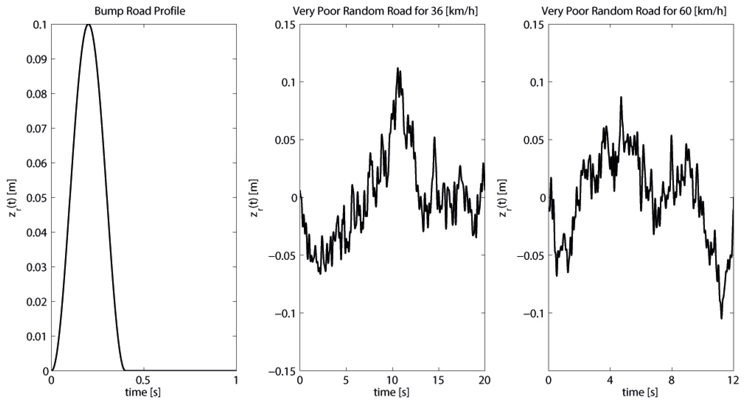
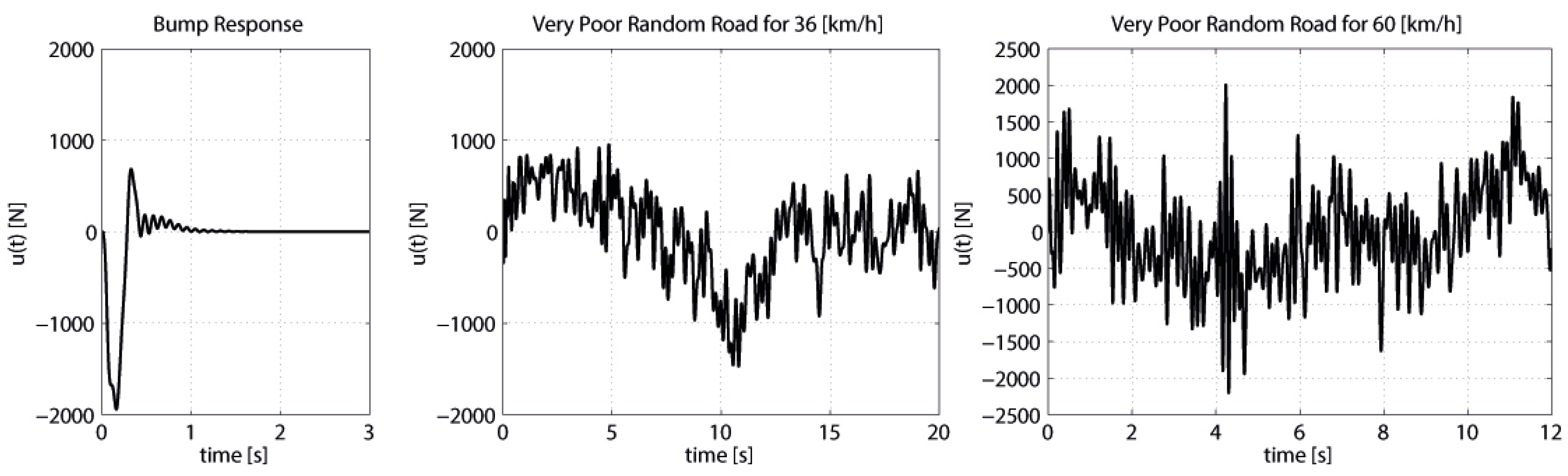
In this study, three typical road profiles are used as disturbance inputs, which are applied to the vehicle wheel. The road bump profile is considered first to reveal the transient response characteristic, which is given by:

$$z_r(t)=\{\begin{array}{ll}\frac{a}{2}(1-\cos (\frac{2\mathsf{\pi }{V}_0}{l}t)),& 0\le t\le \frac{l}{V_0}\\ 0& t\le \frac{l}{V_0}\end{array}$$

(16)

where a and l are height and length of the bump, respectively, and V₀ is the vehicle velocity [6]. Here, road bump profile parameters are chosen as a = 0.1 m, l = 5 m, and V₀ = 45 km/h. Then, ISO2631 very poor random road profile is used as the worst-case disturbance input for the different vehicle velocities [17]. The road disturbance can be considered as the vibration, and it is typically specified as a random process with a ground displacement power spectral density of

$$S_g(\mathsf{\phi })=\{\begin{array}{ll}{S}_g({\mathsf{\phi }}_0){(\frac{\mathsf{\phi }}{{\mathsf{\phi }}_0})}^{-n_1},& if \mathsf{\phi }\le {\mathsf{\phi }}_0\\ S_g({\mathsf{\phi }}_0){(\frac{\mathsf{\phi }}{{\mathsf{\phi }}_0})}^{-n_2},& if \mathsf{\phi }\ge {\mathsf{\phi }}_0\end{array}$$

(17)

where ${\mathsf{\phi }}_0=(1/2\mathsf{\pi })$ is a reference frequency, ϕ is a frequency, and n₁ and n₂ are road roughness constants [17]. The $S_g({\mathsf{\phi }}_0)$ value can be computed by measuring the roughness of the road. The road irregularities can be constructed by the following series, when the vehicle horizontal speed v₀ is assumed to be constant, $z_r(t)={\displaystyle \sum _{n=1}^{N_f}{z}_n\sin (}n{w}_{0}t+{\mathsf{\varphi }}_n)$, where $z_n=\sqrt{2S_g(n\Delta \mathsf{\phi })\Delta \mathsf{\phi }}$, $\Delta \mathsf{\phi }=(2\mathsf{\pi }/l)$, l is the length of the road segment, $w_0=(2\pi /l)v_0$, and ϕ_n are treated as random variables that follow uniform distribution in the interval $[0,2\mathsf{\pi })$. N_f limits the frequency range. The very poor random road profile parameters are chosen according the ISO2631 standards as n₁ = 2, n₂ = 1.5, N_f = 100, l = 200, and $S_g({\mathsf{\phi }}_0)=1024\times {10}^{-6} m^3$. The vehicle velocities are considered as 36 and 60 km/h [17]. The modeled bump and ISO2631 very poor random road disturbances for 36 and 60km/h are shown in Figure 2.

In order to demonstrate the effects of the non-linear characteristics of the spring and damper of the vehicle suspension system, a simulation study is also carried out, which is given in

Table 1. The comparison of the linear and non-linear suspension model using time history responses of cabin floor under very poor random road excitations for 36 and 60 km/h.

Comparison of Linear, Non-Linear Models		Peak to Peak (PP)		RMS Values
		Linear	Nonlinear	Linear	Nonlinear
Very Poor Random Road Profile for 36 (km/h)	z2(t)	0.1942	0.1916	0.0411	0.0408
	${\ddot{z}}_2(t)$	6.0502	6.1436	1.1357	1.1560
Very Poor Random Road Profile for 60 (km/h)	z2(t)	0.2156	0.2073	0.0418	0.0410
	${\ddot{z}}_2(t)$	10.4889	13.3136	1.7557	1.9233

Remark: As can be observed from Table 1, the displacement and acceleration responses of the cabin floor are changed prominently when the vehicle velocity is increased. Additionally, Table 1 reveals that, when the non-linear behaviors of the spring and damper of the suspension system are considered in the controller design, the more realistic results may be obtained for the active suspension control problem. Therefore, the consideration of non-linear behaviors of the suspension spring and damper as the linear parameter-varying (LPV) parameters of the proposed vehicle system within the controller design process provides a more realistic realization of results for the active vibration control of the vehicle suspension system. Due to this result, with this study, a simple realizable synthesis method is introduced to obtain a practically applicable, parameter-dependent optimal state-feedback control law for a parameter-varying vehicle suspension system without utilizing any tuning parameters.

for the comparison of behaviors of the linear and non-linear suspension systems. The linear suspension model can be easily obtained when the non-linear spring and damper parts, $[0.1k_2{(z_2(t)-z_1(t))}^2](z_2(t)-z_1(t))$ and $[0.41c_1\left|{\dot{z}}_2(t)-{\dot{z}}_1(t)\right|]({\dot{z}}_2(t)-{\dot{z}}_1(t))$ are removed from Equations (3) and (4), respectively. The corresponding peak-to-peak vibration amplitude values and RMS values of cabin floor displacement and acceleration responses are compared for both the linear vehicle system and the non-linear vehicle system in Table 1 against the very poor random road disturbance inputs for 36 and 60 km/h.

3. Parameter Dependent Optimal Controller Design for LPV Systems

In this paper, a state-feedback LPV controller is designed to mitigate the vertical vibrations of a non-linear vehicle suspension system. LPV methods have received considerable attention in recent years [18]. LPV-based controller design is a gain-scheduling control method to enable the application of linear methods on the control of non-linear systems. The conventional approach to gain scheduling is a repetitive design procedure with a gridding of an operating domain. Despite the fact that such implementations frequently enjoy success and are deployed in many realistic control systems, conventional techniques provide no guarantee for stability or performance. At this stage, LPV methods guarantee Lyapunov stability and specific performance objectives for non-linear systems [19]. Therefore, to guarantee the closed-loop stability and improve system performance, a LPV-based control algorithm is very suitable for the vibration attenuation of non-linear vehicle suspension systems.

The control objectives are to guarantee the closed-loop stability and disturbance attenuation in the sense of L₂ norm. First, solvability conditions for the L₂ gain controller that depends on the measured scheduling parameters are expressed in terms of a set of LMIs. Then, a coupling constraint is added to the controller design, which fulfills the multiconvexity condition [20]. Consider the following LPV system:

$$\begin{array}{l}\dot{x}(t)=A(\mathsf{\theta })x(t)+B_u(\mathsf{\theta })u(t)+B_w(\mathsf{\theta })w(t)\\ z(t)=C(\mathsf{\theta })x(t)+D_u(\mathsf{\theta })u(t)+D_w(\mathsf{\theta })w(t)\end{array}$$

(18)

where $x(t)\in {\Re }^n$ is the state vector, $u(t)\in {\Re }^{mu}$ is the control input, $w(t)\in {\Re }^{mw}$ is the disturbance input acting on the system, and $z(t)\in {\Re }^p$ is the controlled output. Then, $\mathsf{\theta }=({\mathsf{\theta }}_1,\mathrm{...},{\mathsf{\theta }}_k)\in {\Re }^k$, and $i=1, 2, \mathrm{...}, k$ is a vector of scheduling parameters. The state-space matrices A(θ), B_u(θ), B_w(θ), C(θ), D_u(θ), and D_w(θ) depend affinely on the parameters θ_i. It is assumed that lower and upper bound are available for parameter values and rates of variation. Each parameter θ_i ranges between known extremal values ${\underset{\_}{\mathsf{\theta }}}_i$ and ${\overline{\mathsf{\theta }}}_i$,

$${\mathsf{\theta }}_i\in [{\underset{\_}{\mathsf{\theta }}}_i,{\overline{\mathsf{\theta }}}_i]$$

(19)

This assumption means that the scheduling parameters vector θ is valued in a hyper-rectangle called the parameter box. In the sequel,

$$R_{vex}:=\left\{(w_1,\mathrm{...},w_k):\hspace{1em}{w}_i\in \{{\underset{\_}{\mathsf{\theta }}}_i,{\overline{\mathsf{\theta }}}_i\}\right\}$$

(20)

denotes the set 2^k vertices or corners of this parameter box. The rate of variation ${\dot{\mathsf{\theta }}}_i$ is well defined at all times and satisfies

$${\dot{\mathsf{\theta }}}_i\in [{\underset{\_}{\dot{\mathsf{\theta }}}}_i,{\overline{\dot{\mathsf{\theta }}}}_i]$$

(21)

where ${\underset{\_}{\dot{\mathsf{\theta }}}}_i\le 0\le {\overline{\dot{\mathsf{\theta }}}}_i$ are known lower and upper bounds on ${\dot{\mathsf{\theta }}}_i$. Similarly, Equation (21) delimits on hyper-rectangle of R^k with corners in

$$D_{vex}:=\left\{({\mathsf{\tau }}_1,\mathrm{...},{\mathsf{\tau }}_k): {\mathsf{\tau }}_i\in \{{\underset{\_}{\dot{\mathsf{\theta }}}}_i,{\overline{\dot{\mathsf{\theta }}}}_i\}\right\}$$

(22)

Then, our goal is to design an optimal state-feedback LPV controller that depends on the scheduling parameters θ_i, expressed as $u(t)=K(\mathsf{\theta })x(t)$, which ensures the quadratic stability of the system Equation (18), with a Lyapunov function depending on ${\mathsf{\theta }}_i$’s with a disturbance attenuation level γ. Using this control law, one obtains the closed-loop system as

$$\begin{array}{l}\dot{x}(t)=[A(\mathsf{\theta })+B_u(\mathsf{\theta })K(\mathsf{\theta })]x(t)+B_w(\mathsf{\theta })w(t)\\ z(t)=[C(\mathsf{\theta })+D_u(\mathsf{\theta })K(\mathsf{\theta })]x(t)+D_w(\mathsf{\theta })w\left(t\right)\end{array}$$

(23)

The following theorem presents an optimal state-feedback LPV controller synthesis.

Theorem: 

Consider the closed-loop system Equation (23) with a parameter dependence on θ_i, assume that the parameter trajectories and their derivatives range in hyper-rectangles Equations (20) and (22), and let $R_{vex}$ and $D_{vex}$ denote the corner sets of these hyper-rectangles. For a given non-negative scalar constant, $\mathsf{\gamma }=\sqrt{\mathsf{\mu }}>0$, the closed-loop system Equation (23) is parameter-dependent quadratically stable with the disturbance attenuation level, γ, if there is a positive definite parameter-dependent symmetric matrix $X(\mathsf{\theta })=X{(\mathsf{\theta })}^T$ and a rectangular matrix $L(\mathsf{\theta })$ for each vertex of Equations (20) and (22) subject to

$$\mathrm{\Phi }:=\left[\begin{array}{ccc}\mathrm{\Phi }(\mathsf{\theta },\dot{\mathsf{\theta }})& B_w(\mathsf{\theta })& {(C(\mathsf{\theta })X(\mathsf{\theta })+D_u(\mathsf{\theta })L(\mathsf{\theta }))}^T\\ B_w{(\mathsf{\theta })}^T& -\mathsf{\mu }I& D_w{(\mathsf{\theta })}^T\\ C(\mathsf{\theta })X(\mathsf{\theta })+D_u(\mathsf{\theta })L(\mathsf{\theta })& D_w\left(\mathsf{\theta }\right)& -I\end{array}\right]<0$$

(24)

$$\left[\begin{array}{cc}{A}_i{X}_i+X_i{A}_i^T+B_{ui}{L}_i+L_i^T{B}_{ui}^T+{\mathsf{\eta }}_{i}I& {(C_i{X}_i+D_{ui}{L}_i)}^T\\ C_i{X}_i+D_{ui}{L}_i& {\mathsf{\eta }}_{i}I\end{array}\right]\ge 0,{\forall }_i=1,\mathrm{...},k$$

(25)

and

$$X_0+{\displaystyle \sum _{i=1}^k{\mathsf{\theta }}_i{X}_i}>0,{\mathsf{\theta }}_i\in R_{vex},{\dot{\mathsf{\theta }}}_i\in D_{vex}$$

(26)

where $\mathrm{\Phi }(\mathsf{\theta },\dot{\mathsf{\theta }})=A(\mathsf{\theta })X(\mathsf{\theta })+X(\mathsf{\theta })A{(\mathsf{\theta })}^T+B_u(\mathsf{\theta })L(\mathsf{\theta })+L{(\mathsf{\theta })}^T{B}_u{(\mathsf{\theta })}^T-\dot{X}(\dot{\mathsf{\theta }})$. Then, $\mathsf{\gamma }=\sqrt{\mathsf{\mu }}$ is an L₂ gain of the resulting closed-loop system from $w(t)$ to $z(t)$ for all $t\ge 0$, and the control law $u(t):=L(\mathsf{\theta })X^{-1}(\mathsf{\theta })x(t)$ is an LPV controller associated with γ.

Proof: 

Let us choose an affine quadratic Lyapunov function, $V(x(t),\mathsf{\theta }):=x{(t)}^{T}P(\mathsf{\theta })x(t)$, such that $V(x(t),\mathsf{\theta })>0$ and $\dot{V}(x(t),\mathsf{\theta })<0$ along all admissible parameter trajectories and, for all initial conditions, $x(t_0)=x_0$. Provided that ${\mathsf{\theta }}_i$ and their time derivatives ${\dot{\mathsf{\theta }}}_i$ vary in compact sets, this guarantees asymptotic stability. The closed-loop system Equation (23) is affinely quadratically stable if there is a parameter-dependent symmetric Lyapunov matrix, $P(\mathsf{\theta })=P_0+{\mathsf{\theta }}_1{P}_1+\mathrm{...}+{\mathsf{\theta }}_k{P}_k>0$. Taking the time derivative of $V(x(t),\mathsf{\theta })$ along the system trajectory Equation (23), one obtains

$$\dot{V}(x(t),\mathsf{\theta })=\dot{x}{(t)}^{T}P(\mathsf{\theta })x(t)+x{(t)}^{T}P(\mathsf{\theta })\dot{x}(t)+x{(t)}^T\dot{P}(\mathsf{\theta })x(t)$$

(27)

and

$$\dot{P}(\mathsf{\theta })={\dot{\mathsf{\theta }}}_1{P}_1+\mathrm{...}+{\dot{\mathsf{\theta }}}_k{P}_k=\dot{P}(\mathsf{\theta })-P_0$$

(28)

In addition, closed-loop system Equation (23) has an affine quadratic L₂ gain performance, γ, with the condition

$$\dot{V}(x(t),\mathsf{\theta })+z{(t)}^{T}z(t)-{\mathsf{\gamma }}^{2}w{(t)}^{T}w(t)<0$$

(29)

which holds for all admissible parameter trajectories ${\mathsf{\theta }}_i={\mathsf{\theta }}_1,\mathrm{...},{\mathsf{\theta }}_k$ and ${\dot{\mathsf{\theta }}}_i={\dot{\mathsf{\theta }}}_1,\mathrm{...},{\dot{\mathsf{\theta }}}_k$ for $i=1, 2, \mathrm{...}, k$. Then, substituting the closed-loop system Equation (23) into the condition Equation (29), one obtains

$$\begin{array}{l}{[(A(\mathsf{\theta })+B_u(\mathsf{\theta })K(\mathsf{\theta }))x(t)+B_w(\mathsf{\theta })w(t)]}^{T}P\left(\mathsf{\theta }\right)x(t)\\ +x{(t)}^{T}P(\mathsf{\theta })[(A(\mathsf{\theta })+B_u(\mathsf{\theta })K(\mathsf{\theta }))x(t)+B_w(\mathsf{\theta })w(t)]\\ +x{(t)}^T\dot{P}(\mathsf{\theta })x(t)+x{(t)}^T{(C(\mathsf{\theta })+D_u(\mathsf{\theta })K(\mathsf{\theta }))}^T(C(\mathsf{\theta })+D_u(\mathsf{\theta })K(\mathsf{\theta }))x(t)\\ +w{(t)}^T{D}_w{(t)}^T(C(\mathsf{\theta })+D_u(\mathsf{\theta })K(\mathsf{\theta }))x(t)+x{(t)}^T{(C(\mathsf{\theta })+D_u(\mathsf{\theta })K(\mathsf{\theta }))}^T{D}_w(\mathsf{\theta })w(t)\\ +w{(t)}^T{D}_w{(\mathsf{\theta })}^T{D}_w(\mathsf{\theta })w\left(t\right)-{\mathsf{\gamma }}^2{w}^T(t)w(t)<0\end{array}$$

(30)

On the other hand, let us define an extended state vector as ${\mathsf{\chi }}^T:=[x^T(t) w^T(t)]$. Then, one can easily see that Equation (29) and ${\mathsf{\chi }}^T(t)\Omega \mathsf{\chi }(t)<0$ are equivalent. Hence, if $\Omega <0$ is satisfied, negative definiteness of Equation (29) is also satisfied, where

$$\Omega :=\left[\begin{array}{cc}\begin{array}{c}(A(\mathsf{\theta })+B_u(\mathsf{\theta })K(\mathsf{\theta }))P(\mathsf{\theta })+P(\mathsf{\theta })(A(\mathsf{\theta })+B_u(\mathsf{\theta })K(\mathsf{\theta }))\\ +\dot{P}(\mathsf{\theta })+{(C(\mathsf{\theta })+D_u(\mathsf{\theta })K(\mathsf{\theta }))}^T(C(\mathsf{\theta })+D_u(\mathsf{\theta })K(\mathsf{\theta }))\\ \end{array}& \begin{array}{l}P(\mathsf{\theta })B_w(\mathsf{\theta })\\ +{(C(\mathsf{\theta })+D_u(\mathsf{\theta })K(\mathsf{\theta }))}^T{D}_w(\mathsf{\theta })\\ \end{array}\\ B_w{(\mathsf{\theta })}^{T}P(\mathsf{\theta })+D_w{(\mathsf{\theta })}^T(C(\mathsf{\theta })+D_u(\mathsf{\theta })K(\mathsf{\theta }))& D_w{(\mathsf{\theta })}^T{D}_w(\mathsf{\theta })-{\mathsf{\gamma }}^{2}I\end{array}\right]<0$$

(31)

Applying the Schur complement formula [20] on Equation (31), $\Omega <0$ is congruent to

$$\overline{\Omega }:=\left[\begin{array}{ccc}{\overline{\Omega }}_{11}(\mathsf{\theta },\dot{\mathsf{\theta }})& P(\mathsf{\theta })B_w(\mathsf{\theta })& {(C(\mathsf{\theta })+D_u(\mathsf{\theta })K(\mathsf{\theta }))}^T\\ B_w{(\mathsf{\theta })}^{T}P(\mathsf{\theta })& -{\mathsf{\gamma }}^{2}I& D_w{(\mathsf{\theta })}^T\\ (C(\mathsf{\theta })+D_u(\mathsf{\theta })K(\mathsf{\theta }))& D_w(\mathsf{\theta })& -I\end{array}\right]<0$$

(32)

where ${\overline{\Omega }}_{11}(\mathsf{\theta },\dot{\mathsf{\theta }})={(A(\mathsf{\theta })+B_u(\mathsf{\theta })K(\mathsf{\theta }))}^{T}P(\mathsf{\theta })+P(\mathsf{\theta })(A(\mathsf{\theta })+B_u(\mathsf{\theta })K(\mathsf{\theta }))+\dot{P}(\mathsf{\theta })$. Pre- and post-multiplying Equation (32) by $diag(X(\mathsf{\theta }),I,I)$, where $X(\mathsf{\theta }):=P^{-1}(\mathsf{\theta })$, and applying the variable change $L(\mathsf{\theta }):=K(\mathsf{\theta })X(\mathsf{\theta })$, inequality Equation (32) is congruent to

$$\mathrm{\Phi }:=\left[\begin{array}{ccc}{\mathrm{\Phi }}_{11}(\mathsf{\theta },\dot{\mathsf{\theta }})& B_w(\mathsf{\theta })& {(C(\mathsf{\theta })X(\mathsf{\theta })+D_u(\mathsf{\theta })L(\mathsf{\theta }))}^T\\ B_w{(\mathsf{\theta })}^T& -\mathsf{\mu }I& D_w{(\mathsf{\theta })}^T\\ C(\mathsf{\theta })X(\mathsf{\theta })+D_u(\mathsf{\theta })L(\mathsf{\theta })& D_w(\mathsf{\theta })& -I\end{array}\right]<0$$

(33)

where ${\mathrm{\Phi }}_{11}(\mathsf{\theta },\dot{\mathsf{\theta }})=A(\mathsf{\theta })X(\mathsf{\theta })+X(\mathsf{\theta })A{(\mathsf{\theta })}^T+B_u(\mathsf{\theta })L(\mathsf{\theta })+L{(\mathsf{\theta })}^T{B}_u{(\mathsf{\theta })}^T-\dot{X}(\dot{\mathsf{\theta }})$ with $\mathsf{\gamma }=\sqrt{\mathsf{\mu }}>0$ and

$$X_0+{\displaystyle \sum _{i=1}^k{\mathsf{\theta }}_i{X}_i}>0, {\mathsf{\theta }}_i\in R_{vex}, {\dot{\mathsf{\theta }}}_i\in D_{vex}$$

(34)

As for affine quadratic stability, Equations (33) and (34) put an infinite number of constraints on the unknowns $X_0,\mathrm{...},X_k$. For tractability, Equations (33) and (34) are reduced to a system of finitely many LMIs by imposing multiconvexity. The implications of multiconvexity for scalar quadratic functions are clarified by the following lemma [20].

Lemma [20]: 

Consider a scalar quadratic function of $\mathsf{\theta }\in R^k$,

$$f({\mathsf{\theta }}_1,\mathrm{...},{\mathsf{\theta }}_k)={\mathsf{\alpha }}_0+{\displaystyle \sum _i{\mathsf{\alpha }}_i{\mathsf{\theta }}_i}+{\displaystyle \sum _{i<j}{\mathsf{\beta }}_{ij}{\mathsf{\theta }}_i{\mathsf{\theta }}_j+}{\displaystyle \sum _i{\mathsf{\gamma }}_i{\mathsf{\theta }}_i^2}$$

(35)

and assume that $f(\cdot )$ is multiconvex, that is,

$$2{\mathsf{\gamma }}_i=\frac{{\partial }^{2}f}{\partial {\mathsf{\theta }}_i^2}(\mathsf{\theta })\ge 0 \mathrm{for} i=1,\mathrm{...},k$$

(36)

Then, $f(\cdot )$ is negative in the hyper-rectangle Equation (19) if and only if it takes negative values at the corners of Equation (19): that is, if and only if $f(w)<0$ for all $w$ in the vertex set $R_{vex}$ given by Equation (20). The multiconvexity condition can be constructed by considering the inequality Equation (33) as a quadratic function in the form of Equation (35). Then, inequality Equation (37) is resulted which is equivalent to Equation (36) by the use of the lemma.

$$\left[\begin{array}{cc}{A}_i{X}_i+X_i{A}_i^T+B_{ui}{L}_i+L_i^T{B}_{ui}^T& X_i{C}_i^T+L_i^T{D}_{ui}^T\\ C_i{X}_i+D_{ui}{L}_i& 0\end{array}\right]\ge 0$$

(37)

For clarity, representation of ${\mathrm{\Phi }}_{11}(\theta ,\dot{\theta })<0$ in the form of Equation (35) can be shown:

$$\begin{array}{l}{A}_0{X}_0+X_0{A}_0^T+B_{u0}{L}_0+L_0^T{B}_{u0}^T-{\displaystyle \sum _k{\dot{\mathsf{\theta }}}_k{X}_k}\\ +{\displaystyle \sum _i{\mathsf{\theta }}_i}\left(A_0{X}_i+X_i{A}_0^T+A_i{X}_0+X_0{A}_i^T+B_{u0}{L}_i+L_i^T{B}_{u0}^T+B_{ui}{L}_0+L_0^T{B}_{ui}^T\right)+\\ {\displaystyle \sum _{i<j}{\mathsf{\theta }}_i{\mathsf{\theta }}_j}\left(A_j{X}_i+X_i{A}_j^T+A_i{X}_j+X_j{A}_i^T+B_{uj}{L}_i+L_i^T{B}_{uj}^T+B_{ui}{L}_j+L_j^T{B}_{ui}^T\right)+\\ {\displaystyle \sum _i{\mathsf{\theta }}_i^2}\left(A_i{X}_i+X_i{A}_i^T+A_i{X}_i+X_i{A}_i^T+B_{ui}{L}_i+L_i^T{B}_{ui}^T+B_{ui}{L}_i+L_i^T{B}_{ui}^T\right)<0\end{array}$$

(38)

for all Equations (20) and (22). As it can be observed from Section 2, scheduling parameters are located in only a few entries of the parameter-dependent matrices. Since the matrices, $A_1,\mathrm{...},A_k$, $B_{u1},\mathrm{...},B_{uk}$, $B_{w1},\mathrm{...},B_{wk}$, $C_1,\mathrm{...},C_k$, $D_{u1},\mathrm{...},D_{uk}$, and $D_{w1},\mathrm{...},D_{wk}$ are mostly low ranked, strict inequalities are not constituted easily. A simple solution to this numerical problem is proposed in [20]. By implanting non-negative scalars ${\mathsf{\eta }}_i$ into Equation (37), Equation (25) is obtained. This completes the proof.

4. Numerical Simulation Study

In this section, an extensive number of simulations are carried out to illustrate the effectiveness of the proposed controller. To improve the driver’s ride comfort and essential performance requirement, a parameter-dependent optimal controller is designed which is scheduling online according to suspension stroke and its variation rate. To ensure that both responses are within permissible limits, the performance output vector z(t) is constructed as

$$z(t)=C(\mathsf{\theta })x(t)+D_u(\mathsf{\theta })u(t)+D_w(\mathsf{\theta })w(t)$$

(39)

where $C(\mathsf{\theta })=C_0+{\mathsf{\theta }}_1{C}_1+{\mathsf{\theta }}_2{C}_2$, $D_{zu}(\mathsf{\theta })=D_{u0}+{\mathsf{\theta }}_1{D}_{u1}+{\mathsf{\theta }}_2{D}_{u2}$, $D_w(\mathsf{\theta })=D_{w0}+{\mathsf{\theta }}_1{D}_{w1}+{\mathsf{\theta }}_2{D}_{w2}$, $C_0=[\begin{array}{ccc}{0}_{4\times 1}& I_4& 0_{4\times 5}\end{array};A(6, 1-10);A(10, 1-10);\begin{array}{ccc}-1& 1& 0_{1\times 8}\end{array};\begin{array}{cc}1& 0_{1\times 9}\end{array}]$, $C_1=[0_{4\times 10};\begin{array}{ccc}1/m_2& -1/m_2& 0_{1\times 8}\end{array};0_{3\times 10}]$, $C_2=[0_{4\times 10};\begin{array}{cccc}{0}_{1\times 5}& 1/m_2& -1/m_2& 0_{1\times 3}\end{array};0_{3\times 10}]$, $D_{u0}=[0_{6\times 1};1/m_2;0_{3\times 1}]$, $D_{u1}=D_{u2}=0_{8\times 1}$, $D_{w0}=[0_{7\times 1};-1]$ and $D_{w1}=D_{w2}=0_{8\times 1}$. These matrices are chosen to represent the following variables:

$$z(t)={[\begin{array}{cccccccc}{z}_2(t)& z_3(t)& z_4(t)& z_5(t)& {\ddot{z}}_2(t)& {\ddot{z}}_5(t)& z_2(t)-z_1(t)& z_1(t)-z_r\end{array}(t)]}^T$$

(40)

as a specified performance output vector. To achieve a minimum L₂ gain from w(t) to z(t) for all $t\ge 0$, the proposed theorem is applied to this problem, and the minimum allowable disturbance attenuation level γ is calculated as 14.72 and a parameter-dependent optimal state-feedback control law is constructed as $u(t)=L(\mathsf{\theta })X{(\mathsf{\theta })}^{-1}x(t)$, where $L(\mathsf{\theta })=L_0+{\mathsf{\theta }}_1{L}_1+{\mathsf{\theta }}_2{L}_2$ and $X(\mathsf{\theta })=X_0+{\mathsf{\theta }}_1{X}_1+{\mathsf{\theta }}_2{X}_2$. In order to demonstrate the proposed controller performance, bump and very poor random road irregularities are used as the disturbance input as modeled in Section 2 and shown in Figure 2.

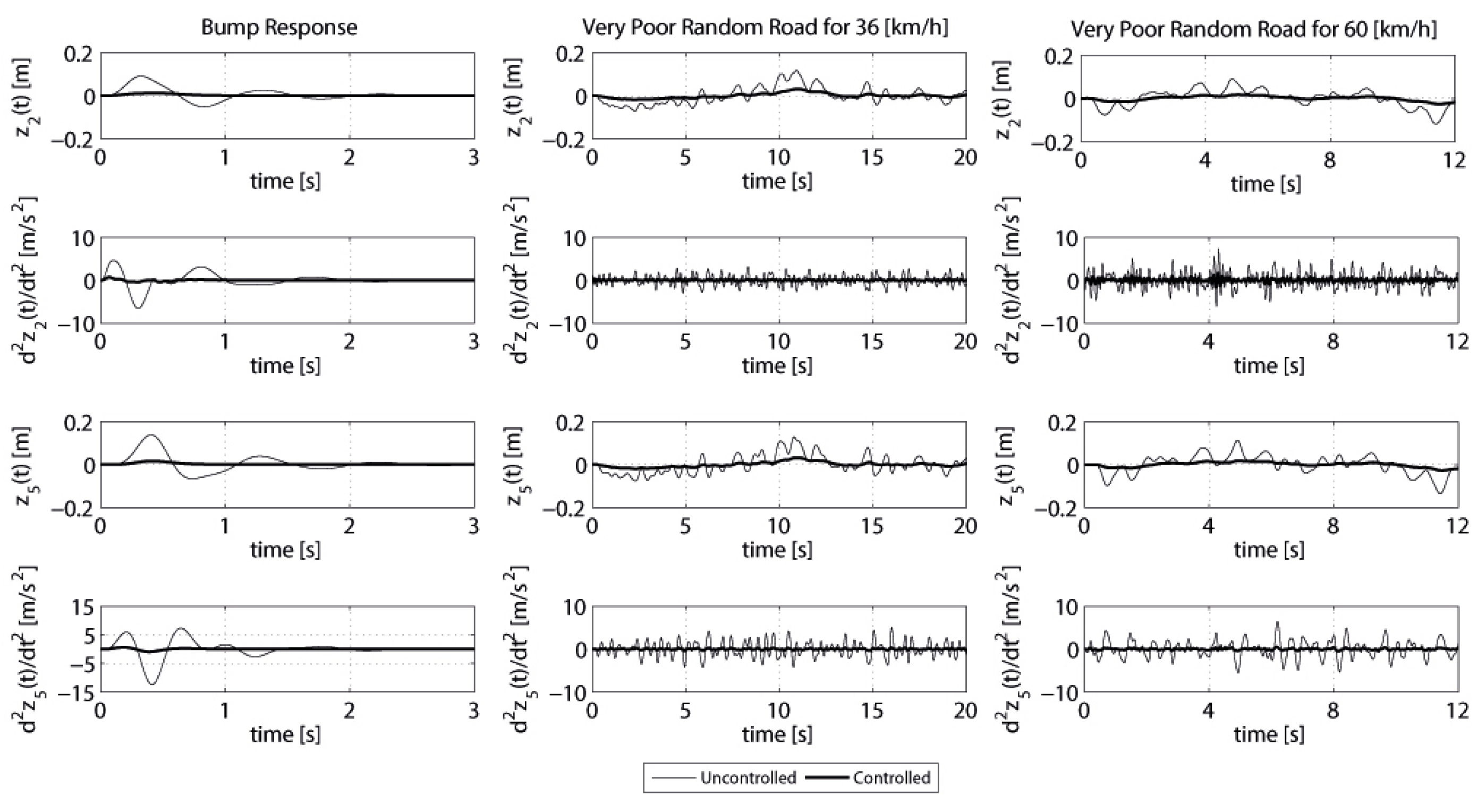
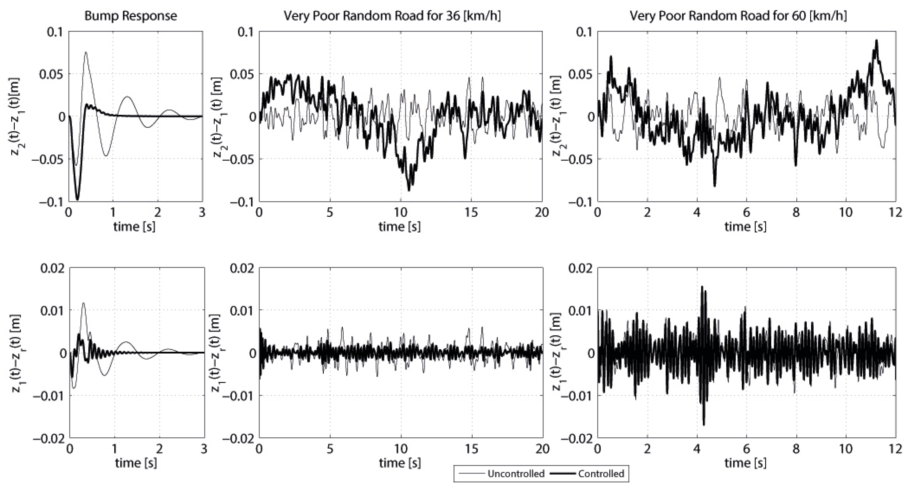
Figure 3 shows the time responses of the vertical displacements and accelerations of cabin floor and driver body of the considered vehicle system, respectively. As can be observed from this figure, very successful vibration suppression is achieved by the use of the designed controller. Note that the designed controller achieves good control performance on ride comfort in terms of the peak value of driver body acceleration.

To evaluate the proposed controller performance on different performance aspects, vehicle suspension stroke and tire deflection properties are shown in Figure 4. This figure reveals that the designed controller has a satisfactory control performance and achieves a good trade-off.

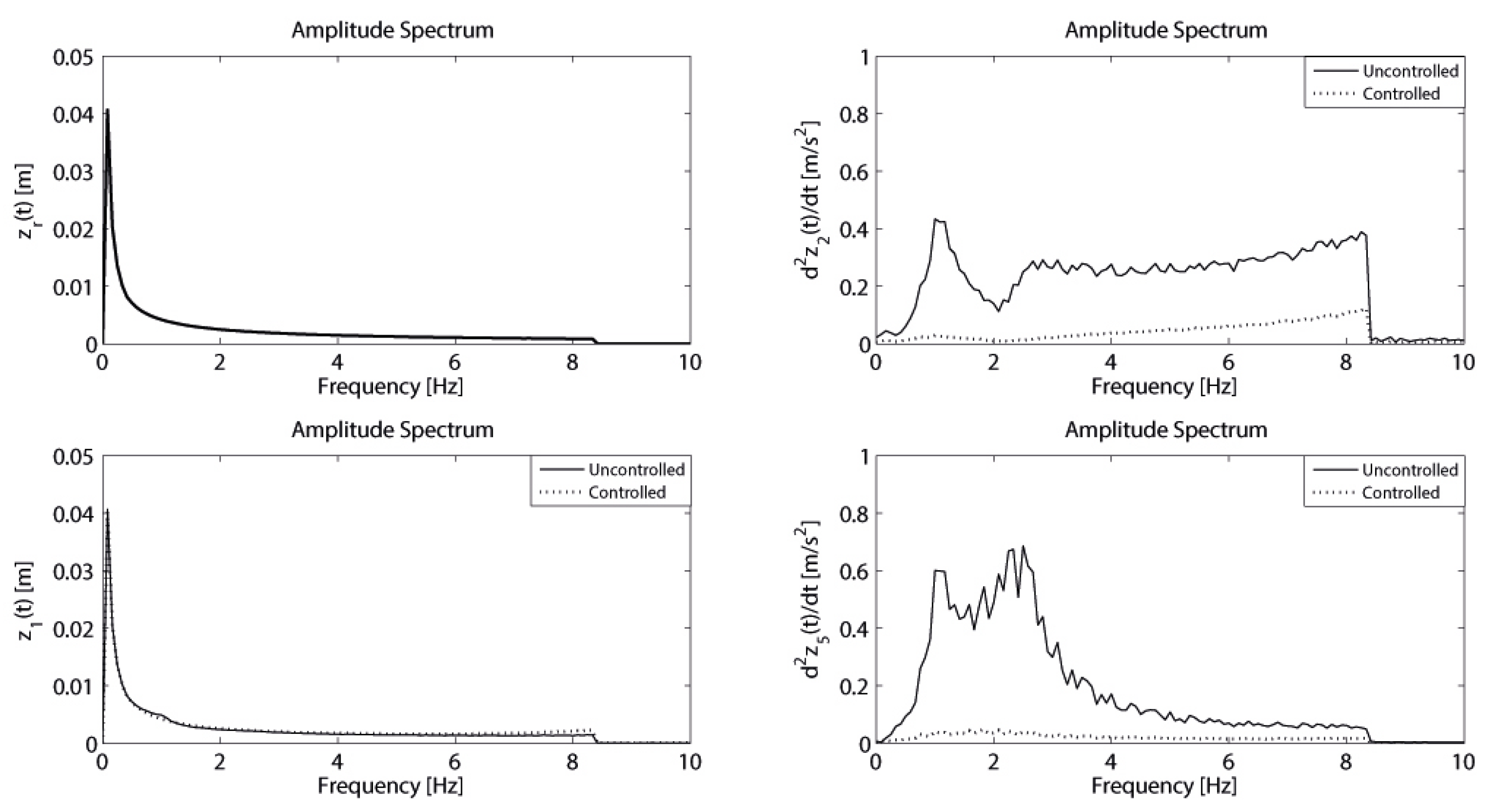
Figure 5 demonstrates the amplitude spectrum plots of displacement of the very poor random road profile, as well as displacement responses of the vehicle wheel and acceleration responses of the cabin floor and driver body for both controlled and uncontrolled cases under very poor random road excitation at 60 km/h.

As expected, frequency content of the z_r(t) for 60 km/h is limited to 8.33 Hz. Note that computation of random road roughness is based on the summation of different sine waves as $z_r(t)={\displaystyle \sum _{n=1}^{N_f}{z}_n\sin (}n{w}_{0}t+{\mathsf{\varphi }}_n)$. Upper bound of the frequency content can be easily obtained by the multiplication of nw₀, where the upper bound of the n is given as 100 and $w_0=(2\mathsf{\pi }/l)v_0$ takes the value of 0.5236 for l = 200 m and v₀ = 16.67 m/s. Therefore, the maximum value of the nw₀ is 52.36 rad/s and 8.33 Hz.

As can be seen from Figure 5, there is no degradation in the performance of the closed-loop control system when the displacement response plot of the vehicle wheel with controlled and uncontrolled cases is compared. Note that the proposed controller largely reduces the cabin floor and driver body accelerations compared to the uncontrolled system and therefore achieves a very successful ride comfort performance.

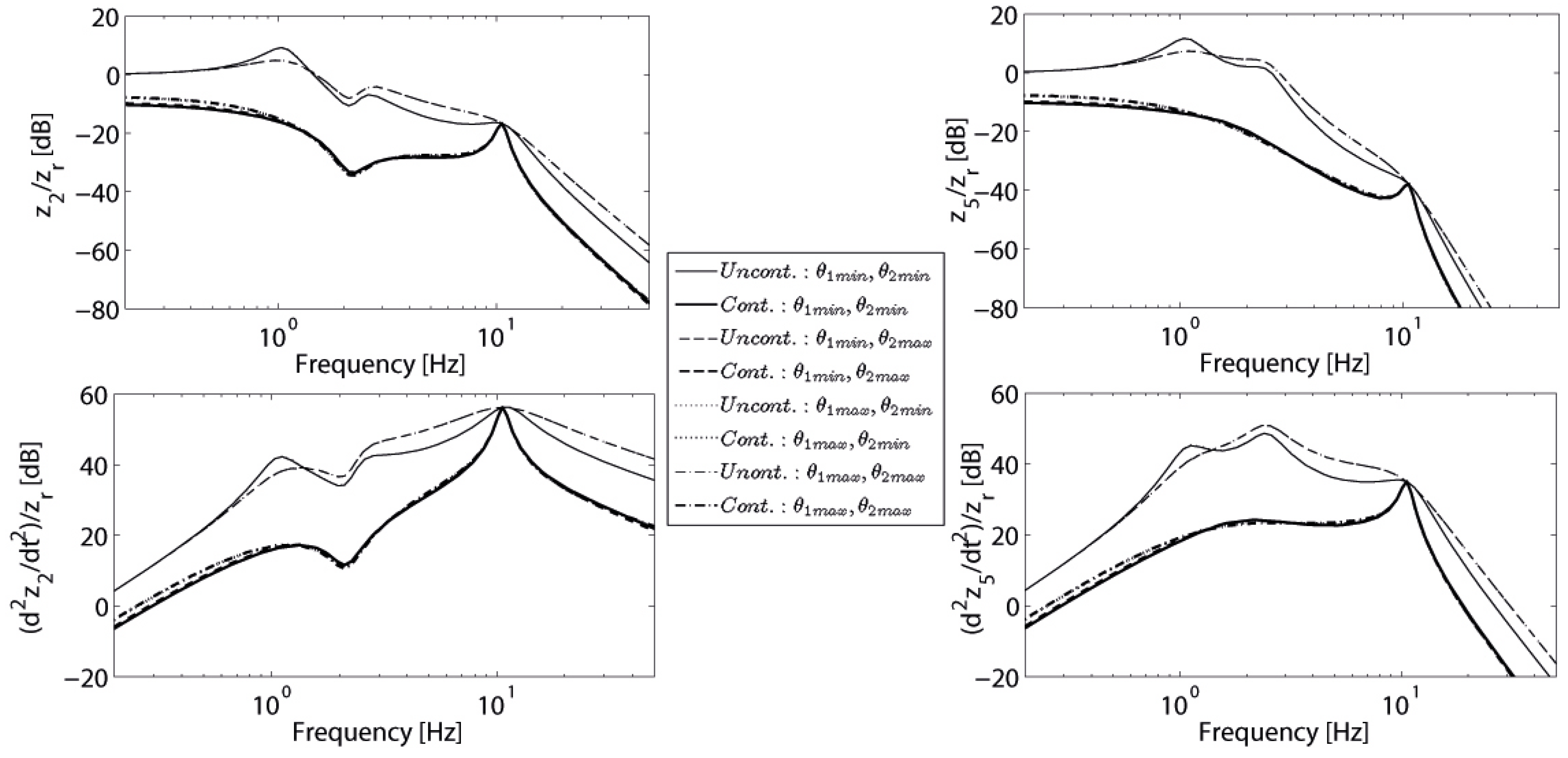
As is mentioned in Section 3, the parameter-dependent controller design for the LPV system is a kind of gain-scheduling control method. In this method, the value of the controller gain matrix of the proposed controller does not remain fixed while the controller is in operation; rather, it is modified in accordance with the scheduling parameters. Therefore, the frequency responses can be obtained by assuming that time-varying parameters are frozen for their vertex points. Figure 6 shows the frequency responses of the displacements and accelerations of the cabin floor and driver body, respectively, for both controlled and uncontrolled cases when the frozen scheduling parameters for their vertex points are considered. As expected, high gain responses belong to the uncontrolled system. When the response plots of the system with uncontrolled and controlled cases are compared, a superior improvement in the mitigation of the resonance values is obtained by the proposed controller. On the other hand, Figure 7 demonstrates that the change in control forces the inputs for the bump and very poor random road excitations. As can be observed from this figure, the applied control forces, which range within maximum ±2200 N for the worst-case road excitations, are very suitable to produce for practical implementations, as discussed in [6,10,11].

In this section, the root mean square (RMS) value, which is the statistic measure of the magnitude of varying quantity, is employed to investigate the active suspension performance. The RMS analysis method is very useful for evaluating active control performance when the variants are positive and negative [6]. The corresponding RMS values of the vertical cabin floor, driver body displacement, acceleration responses, suspension stroke, and tire deflection responses are compared for both the controlled and uncontrolled cases in

Table 2. Comparison of RMS values of the vertical cabin floor and driver body displacement and acceleration responses, suspension stroke, and tire deflection responses.

RMS Values	Bump		Very Poor Random Road for 36 (km/h)		Very Poor Random Road for 60 (km/h)
	Uncontrolled	Controlled	Uncontrolled	Controlled	Uncontrolled	Controlled
z2(t)	0.0299	0.0043	0.0408	0.0114	0.0410	0.0109
z5(t)	0.0407	0.0049	0.0439	0.0116	0.0447	0.0110
${\ddot{z}}_2(t)$	1.6877	0.1436	1.1560	0.1347	1.9233	0.3866
${\ddot{z}}_5(t)$	3.1507	0.2313	1.7388	0.1393	2.0037	0.1706
$z_2(t)-z_1(t)$	0.0249	0.0213	0.0156	0.0281	0.0178	0.0299
$z_1(t)-z_r(t)$	0.0032	0.0010	0.0020	0.0010	0.0038	0.0040

for the bump and very poor random road disturbance inputs at different velocities, respectively.

5. Conclusions

This paper presents an approach for designing a parameter-dependent optimal controller to mitigate the vertical vibration occurring in non-linear vehicle suspension systems with an integrated seat and driver body model. Using parametric Lyapunov functions, the solvability conditions for the design parameter-dependent optimal state-feedback controller that depend on the measured non-linear suspension parameters are expressed in terms of LMIs and an additional constraint which overtakes the convexity problem. The main purpose of this study is to develop an easily realizable synthesis method to obtain a practically applicable parameter-dependent state-feedback controller that provides the best performance while also taking the non-linear behaviors of the suspension spring and damper into account, without utilizing any tuning parameters. Numerical simulations are used to show the performance of the proposed controller. Simulation results indicate that the proposed controller is completely effective in reducing vertical vibration amplitudes of the modeled vehicle system and provides satisfactory ride comfort, suspension stroke, and tire deflection performances. Expanding the proposed method with a parameter-dependent optimal controller design under the consideration of actuator dynamics, actuator saturation, and active seat suspension might be a direction of future work.