Numerical Simulation Study on the Flow Field Out of a Submerged Abrasive Water Jet Nozzle

Abstract

In order to optimize the parameters of pre-mixed abrasive water jet cutting technology, make it more efficient in the coal mine gas environment and solve the problem of hard coal and the difficulty of rock drilling, FLUENT software was used to get the isothermal, incompressible, steady flow field out of a submerged abrasive water jet nozzle through numerical simulation, with different particle sizes and different confining pressures under submerged conditions. The results show that, under submerged conditions, the maximum velocity of the abrasive particle outside the pre-mixed abrasive water jet nozzle is about 6 mm far away from the nozzle; the abrasive particle diameter has little influence on the velocity outside the nozzle. The external confining pressure of the nozzle has an important influence on the velocity, which is that the jet velocity of the same position decreases with the increase of confining pressure and the relationship between the confining pressure of different distance from the nozzle exit and the abrasive velocity is exponential function. The results of the simulation laid the foundation for optimizing the nozzle structure, improving efficiency and developing the abrasive water jet nozzle.

1. Introduction

Abrasive water jet (AWJ) cutting is closely related to safety engineering [1,2]. AWJ cutting is the “cold cutting” that cannot produce heat during the cutting process, so it is particularly fit for the work of cutting in flammable and explosive environments for safety. In mines, there are many demands for cutting rock, bolt and other metal materials. The pre-mixed abrasive water jet that helps in drilling and the coal slotted relief adopted in the field of coal are efficient technical methods for improving the pre-pumping effect of low permeability coal seam gas. The method of abrasive water jet breaking of coal and rock was studied by Li [3]. The technology used in the field of coal was proven safe through the acceleration mechanism of pre-mixed abrasive jets used in cutting safely studied by Li and Guo [4]. In recent years, the technology and equipment for high-pressure abrasive jet cutting, drilling and penetration enhancing were studied and applied in Ping Ding Shan Coal Group by Lin [5]. Significant research was carried out on the aspects of abrasive water jet cutting and drilling to prevent coal and gas outbursts. The technology of high-pressure abrasive water jet cutting was developed and applied to the seam roadway heading face for application testing by Li [6].

With the development of computer technology and computational mathematics, fluid computing software has been developed that makes it possible to analyze high-speed complex liquid. The flow field out of the submerged abrasive water jet nozzle is a kind of typical turbulent two-phase flow with liquid and solid.

The numerical simulation of the external flow field of the nozzle was carried out under submerged conditions by Liu Lifang et al. [7,8]. The numerical simulation of abrasive water jets was carried out based on the theory of continuous medium, and the main parameters of the model were optimized by Wang Mingbo et al. [9,10,11]. PHOENICS software was used to simulate the distribution of the flow field of submerged abrasive jets in deep water by Gao Jifei et al. [12]. In this thesis, the liquid-solid two-phase flow field out of the submerged abrasive water jet nozzle will be simulated using the numerical simulation method. The achievements can provide the basis for optimizing AWJ cutting equipment in mines.

2. Mathematical Model

For solving the problem of liquid-solid two-phase flow in the external field of pre-mixed abrasive water jet through FLUENT software, the following steps should be followed: (1) dividing the grid, establishing the calculating model; (2) determining the boundary conditions; (3) determining the numerical method; (4) conducting the flow solution; (5) outputting the diagram of the relationship between the velocity and the displacement of the solid and liquid phase.

2.1. Main Assumptions

The flow field out of the submerged abrasive water jet nozzle is a kind of liquid-solid two-phase flow [13]. Particle fraction in volume for pre-mixed AWJ is generally less than 15%. Therefore, the Lagrange discrete model is used and liquid will be treated as continuous phase that is described by the Euler coordinates, and then the flow field will be attained through direct solution of Reynolds time-averaged Navier-Stokes equations. The abrasive particles will be treated as discrete phase and described in the Lagrange coordinates, the motion trajectory will be found by calculating the motion rules of particles in the flow field.

Basic hypothesis: (1) As a continuous medium, water is incompressible; (2) there is no mass exchange between abrasive and water; (3) there is no external heat exchange after the mixture of the abrasive and water and the temperature will not change.

2.2. Governing Equations [14,15,16,17,18,19,20]

The Euler model is used in the text; in the meantime, in order to describe the multiphase flow, the volume fraction of the phase is introduced

$$V_q={\displaystyle {\int }_V{\partial }_q}dV$$

(1)

$${\displaystyle \sum _{q=1}^n{\partial }_q}=1$$

(2)

$${\stackrel{⌢}{\mathsf{\rho }}}_q={\partial }_q{\mathsf{\rho }}_q$$

(3)

where ${\partial }_q$ is the volume fraction of q phase; $V_q$ is the volume of q phase; ${\stackrel{⌢}{\mathsf{\rho }}}_q$ is the effective density of q phase; ${\mathsf{\rho }}_q$ is the density of q phase.

The continuous equation and the momentum equation of Euler model are as follows:

(1) Continuous equation:

$$\frac{\mathsf{\alpha }}{{\mathsf{\alpha }}_t}\left({\mathsf{\alpha }}_q{\mathsf{\rho }}_q\right)+\nabla \left({\mathsf{\alpha }}_q{\mathsf{\rho }}_q{\mathsf{\nu }}_q\right)={\displaystyle \sum _{i=1}^n\stackrel{•}{m_{iq}}}$$

(4)

where ${\mathsf{\nu }}_q$ is the velocity of q phase; ${\partial }_q$ is the volume fraction of q phase; ${\mathsf{\rho }}_q$ is the density of q phase; t- time; $\stackrel{•}{m_{iq}}$ is the mass transfer from phase i to phase q;

$$\stackrel{•}{m_{iq}}=-\stackrel{•}{m_{qi}}$$

(5)

$$\stackrel{•}{m_{ii}}=0$$

(6)

(2) Momentum equation

$$\frac{\partial }{{\partial }_t}\left({\partial }_q{\mathsf{\rho }}_q{\mathsf{\nu }}_q\right)+\nabla \left({\partial }_q{\mathsf{\rho }}_q{\mathsf{\nu }}_q^2\right)=-{\partial }_q\nabla \mathsf{\rho }+\nabla {\mathsf{\tau }}_q+{\displaystyle \sum _{i=1}^n\left(R_{iq}+{\stackrel{•}{m}}_{iq}{\mathsf{\nu }}_{iq}\right)+}{\partial }_q{\mathsf{\rho }}_q\left(F_q+F_{lift,q}+F_{vm,q}\right)$$

(7)

where, ${\mathsf{\tau }}_q$ is the pressure strain tensor of q phase here:

$${\mathsf{\tau }}_q={\partial }_q{\mathsf{\mu }}_q\left(\nabla v_q^{\mathsf{\tau }}\right)+{\partial }_q\left({\mathsf{\lambda }}_q-\frac{2}{3}{\mathsf{\mu }}_q\right)\nabla v_{q}I$$

(8)

where, ${\mathsf{\mu }}_q$ is shear viscosity of q phase; ${\mathsf{\lambda }}_q$ is bulk viscosity of q phase; $F_q$ is virtual mass force of q phase; $P$ is the pressure all phases share; $I$ is the unit strain tensor; $R_{iq}$ is interaction force between phases; ${\mathsf{\nu }}_{iq}$ is interphase velocity;

The force between each phase is $R_{iq}$, which meets the following formula:

$${\displaystyle \sum _{i=1}^n{R}_{iq}}={\displaystyle \sum _{i=1}^n{K}_{iq}}\left(v_i-v_q\right)$$

(9)

The momentum exchange coefficient of interphase $K_{iq}=K_{qi}$.

The lift $F_{\text{lift}}$ meets:

$$F_{\text{lift}}=-0.5{\partial }_q{\mathsf{\rho }}_q\left(v_q-v_i\right)x\left(\nabla v_q\right)$$

(10)

$$F_{\text{lift},\mathrm{q}}=-F_{\text{lift},\mathrm{i}}$$

(11)

The virtual mass force meets:

$$F_{\text{Vm}}=0.5{\partial }_i{\mathsf{\rho }}_q\left(\frac{d_q{v}_q}{dt}-\frac{d_i{v}_i}{dt}\right)$$

(12)

$$\frac{d_q\left(\mathsf{\varphi }\right)}{dt}=\frac{\partial \mathsf{\varphi }}{\partial t}+\left(v_q\nabla \right)\mathsf{\varphi }$$

(13)

$$F_{\text{Vm},\mathrm{q}}=-F_{\text{Vm},\mathrm{i}}$$

(14)

(3) Exchange coefficient between liquid and solid:

$$K_{sl}=\frac{{\partial }_s{p}_{s}f}{{\mathsf{\tau }}_s}$$

(15)

where ${\partial }_s$ is the relaxation time of the particles:

$${\mathsf{\tau }}_s=\frac{p_s{d}_s^2}{18{\mathsf{\mu }}_l}$$

(16)

where $K_{sl}$ is the exchange coefficient between liquid and solid; $d_s$ is the diameter of $s$ particles; $f$ is drag function.

2.3. Standard $K-\mathsf{\epsilon }$ Turbulence Equations

For the flow of abrasive water jet, standard $K-\mathsf{\epsilon }$ turbulence equations was adopted in this text.

Turbulent kinetic energy equation:

$$\frac{\partial \left(pk\right)}{\partial t}+\frac{\partial }{\partial x_i}\left(p{U}_{i}k\right)=\frac{\mathsf{\alpha }}{\partial x_j}\left[\left(\mathsf{\mu }+\frac{{\mathsf{\mu }}_i}{{\mathsf{\sigma }}_k}\right)\frac{\mathsf{\alpha }k}{\mathsf{\alpha }{x}_j}\right]+{\mathsf{\mu }}_j\left(\frac{\mathsf{\alpha }{U}_i}{\mathsf{\alpha }{x}_j}+\frac{\mathsf{\alpha }{U}_j}{\mathsf{\alpha }{x}_j}\right)\frac{\mathsf{\alpha }{U}_i}{\mathsf{\alpha }{x}_j}-p\mathsf{\epsilon }$$

(17)

Turbulent energy dissipation rate equation:

$$\frac{\partial \left(p\mathsf{\epsilon }\right)}{\partial t}+\frac{\partial }{\partial x_i}\left(p{U}_i\mathsf{\epsilon }\right)=\frac{\mathsf{\alpha }}{\partial x_j}\left[\left(\mathsf{\mu }+\frac{{\mathsf{\mu }}_t}{{\mathsf{\sigma }}_{\mathsf{\epsilon }}}\right)\frac{\mathsf{\alpha }\mathsf{\epsilon }}{\mathsf{\alpha }{x}_j}\right]+C_{1\mathsf{\epsilon }}{\mathsf{\mu }}_t\left(\frac{\mathsf{\alpha }{U}_i}{\mathsf{\alpha }{x}_j}+\frac{\mathsf{\alpha }{U}_j}{\mathsf{\alpha }{x}_i}\right)-p{C}_{2\mathsf{\epsilon }}\frac{{\mathsf{\epsilon }}^2}{k}$$

(18)

where ${\mathsf{\mu }}_t$ is turbulent viscosity:

$${\mathsf{\mu }}_t=p{C}_{\mathsf{\mu }}\frac{k^2}{\mathsf{\epsilon }}$$

(19)

where $k$ is turbulent kinetic energy; $\mathsf{\epsilon }$ is the turbulent kinetic energy dissipation rate; ${\mathsf{\sigma }}_k$ is the corresponding turbulence Prandtl number of k; ${\mathsf{\sigma }}_{\mathsf{\epsilon }}$ is the corresponding turbulence Prandtl number of $\mathsf{\epsilon }$; $U_i$ is the speed of $x_j$ direction; $U_j$ is the speed of $x_j$ direction; $C_{\mathsf{\mu }}$ is the empirical constant; $C_{1\mathsf{\epsilon }}$ is coefficient; $C_{2\mathsf{\epsilon }}$ is coefficient. The constant values here are $C_{\mathsf{\mu }}=0.09$, $C_{1\mathsf{\epsilon }}=1.44$, $C_{2\mathsf{\epsilon }}=1.92$, ${\mathsf{\sigma }}_k=1.0$, ${\mathsf{\sigma }}_{\mathsf{\epsilon }}=1.3$.

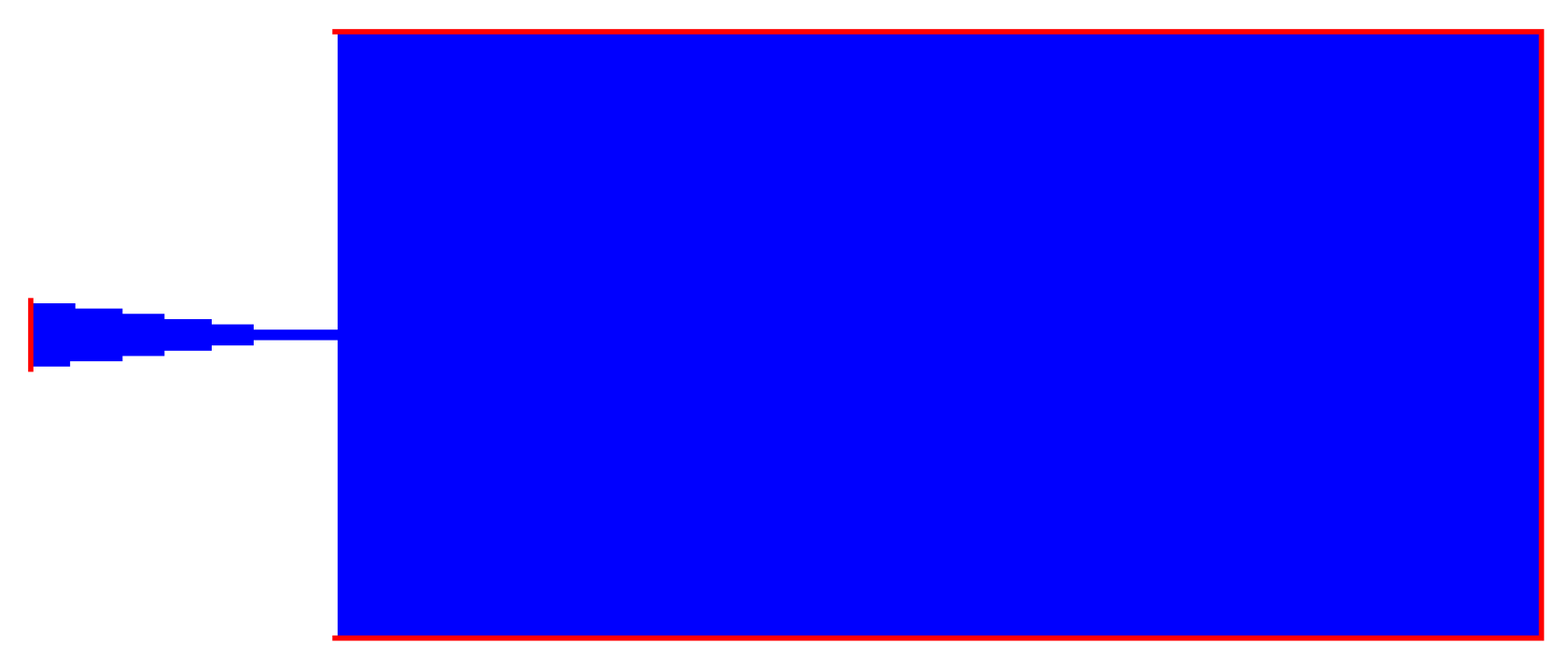
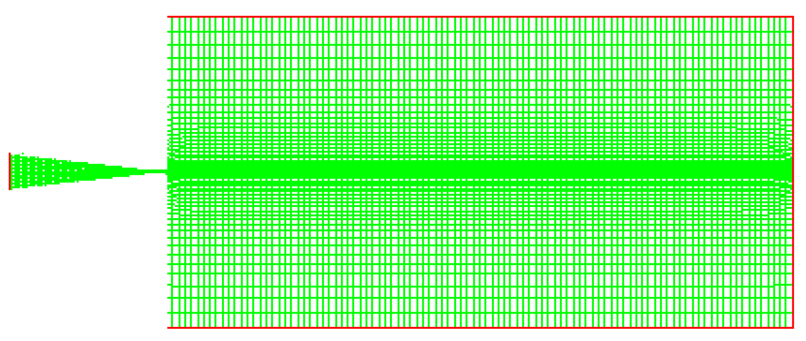
2.4. Geometrical Model

The pre-processing software Gambit was adopted to build the physical model and finish the mesh generation. The main parameters of the physical model: the diameter of the nozzle exit is 1 mm, the length of cylindrical section is 3 mm, the diameter of the nozzle entry d is 6 mm, the total length of the nozzle is 24.94 mm. The dimension of the external zone of the nozzle is 50 mm×100 mm, on which the physical model shown in Figure 1 is based.

In order to optimize the simulation effect, the inner and outer jet center regional mesh of the nozzle was encrypted and, as is shown in Figure 2, this grid resolution is sufficient to properly describe the flow of computing domain, the good effect of abrasive particle size and find the confining pressure on the jet flow field.

2.5. Boundary Conditions

The inlet boundary of the nozzle is set as the pressure inlet, the outlet boundary of the nozzle is set as the pressure outlet, the solid wall is satisfied with no slip condition, and the near wall region is treated by the wall function method.

Because of the high flow velocity, the water and abrasive will provide the irregular movement in the nozzle and the jet area. Therefore, the standard k-ε turbulence model was used for the simulation of irregular flow field and a phase coupled SIMPLE algorithm was used as the solving method. The setting of material properties when calculating was as follows: the first phase medium is water, whose density is 1000 kg/m³ and viscosity is 0.001 Pa·s; the second is garnet, whose density is 2300 kg/m³ and viscosity is 0.001 Pa·s.

3. Results and Analysis

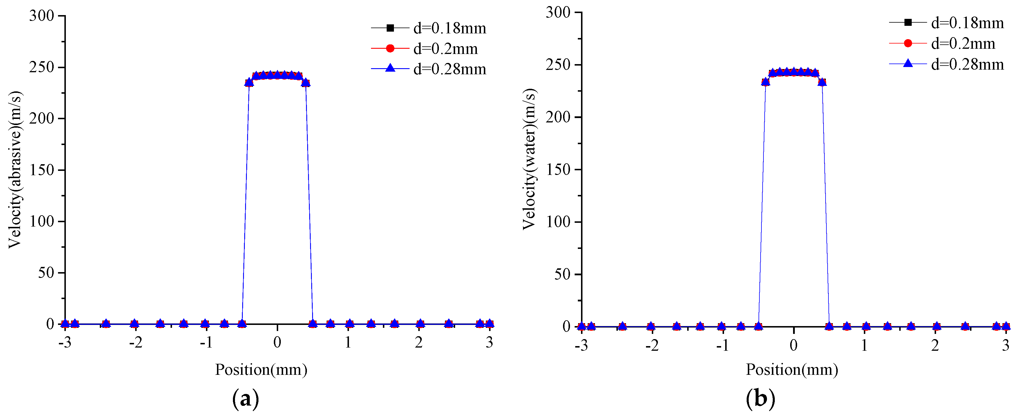
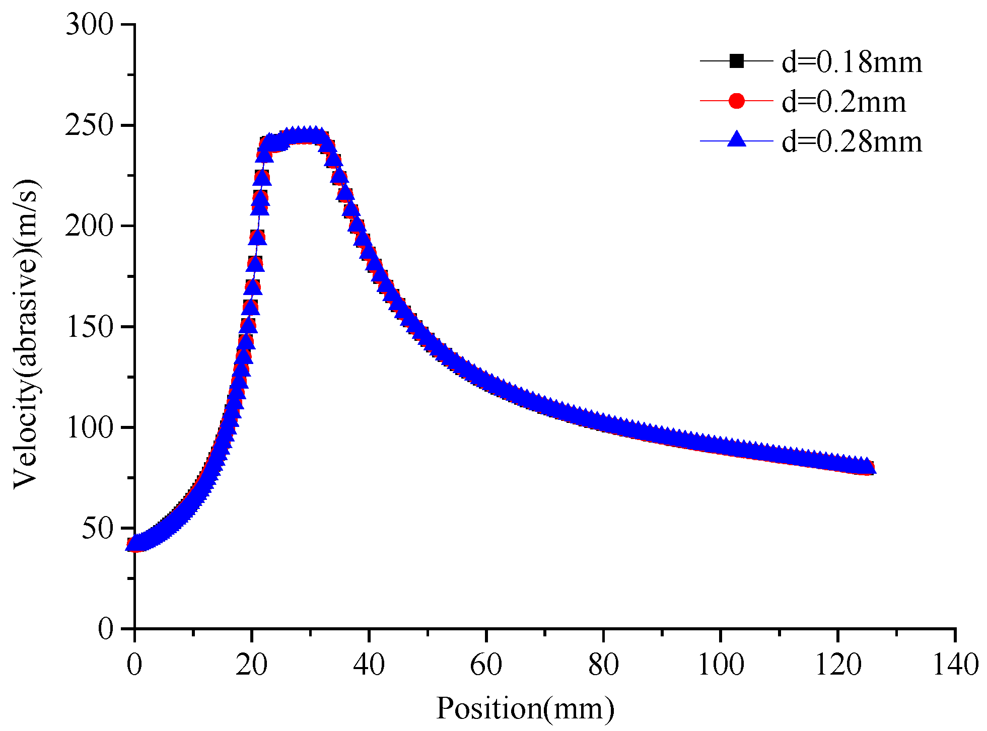
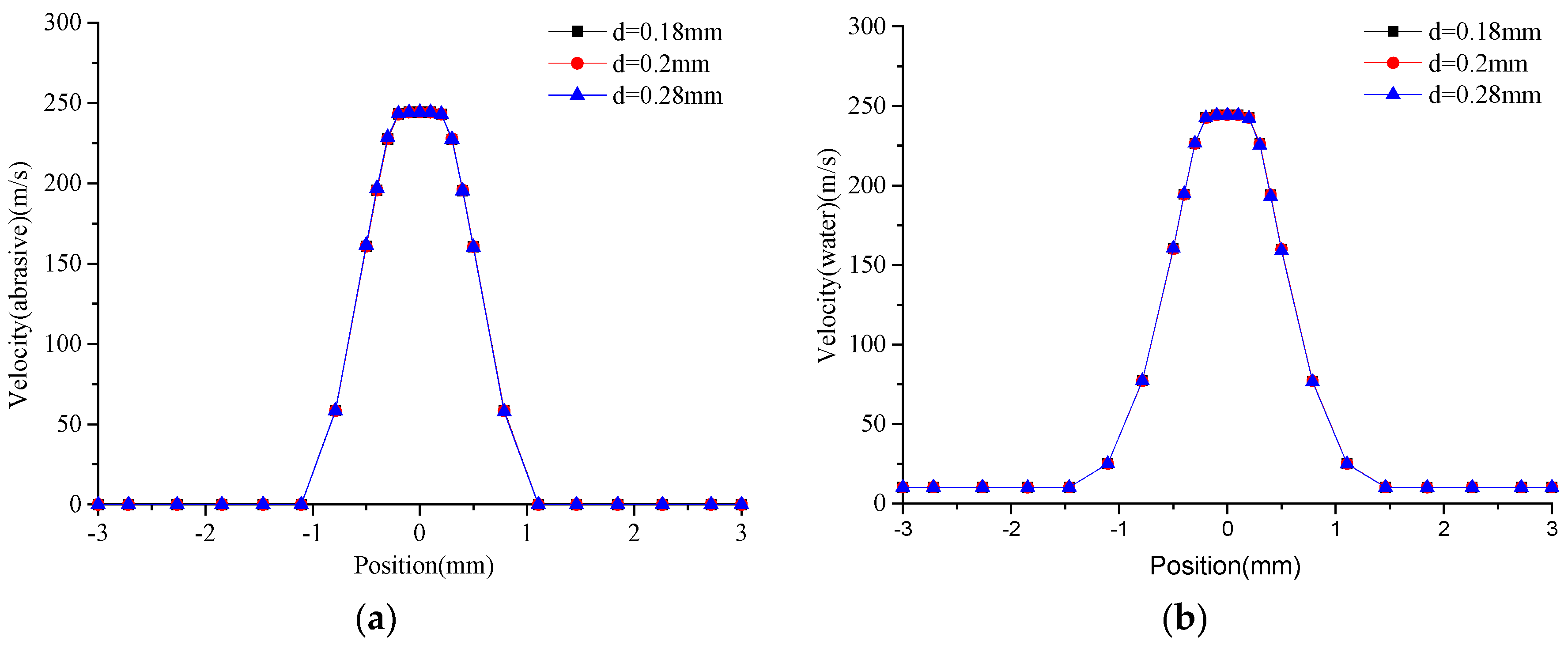
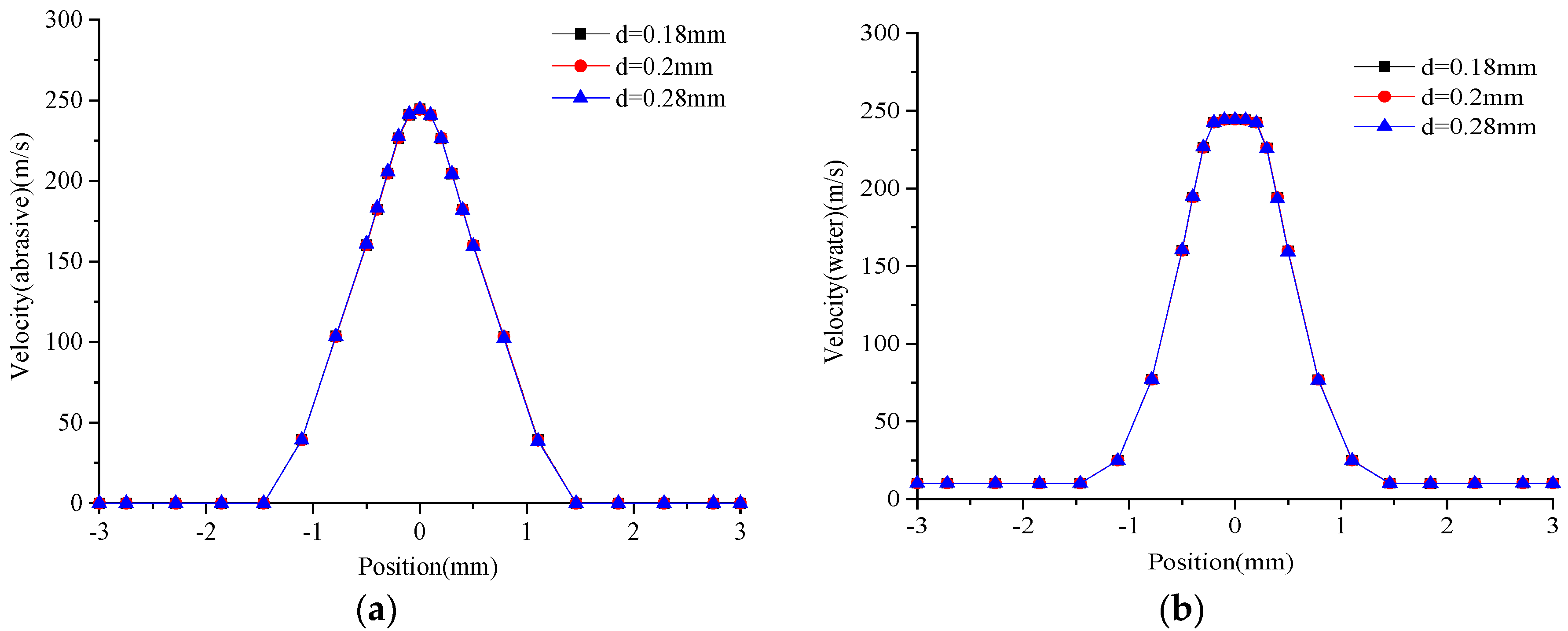
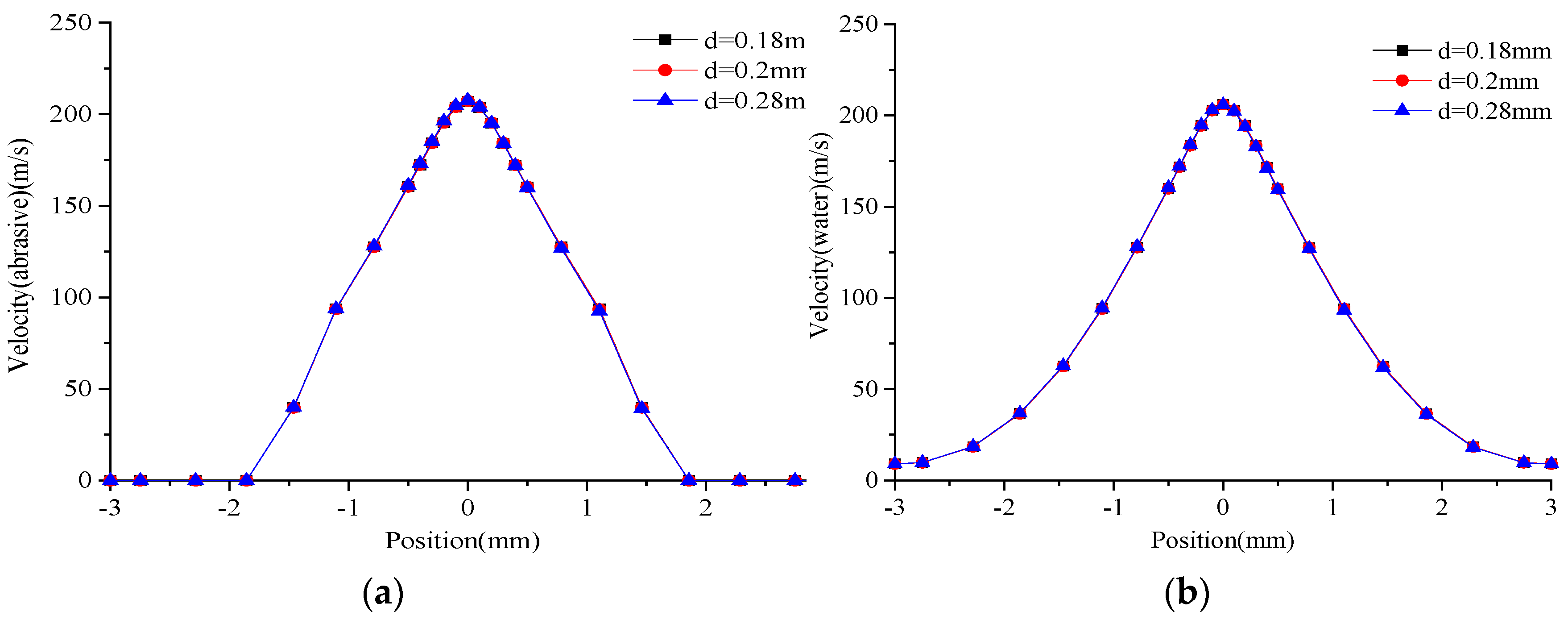
3.1. The Effect of Abrasive Particle Sizes on the Jet Flow Field

The influence of different abrasive particle sizes on the distribution of the jet flow field was considered in the condition that the confining pressure was 0 MPa, the abrasive concentration was 10% and the inlet pressure was 30 MPa. The numerical simulation method was used to simulate the jet flow field when the size of the abrasive particle were 0.28 mm, 0.2 mm and 0.18 mm, respectively.

(1)

Axial velocity distribution

Figure 3 is the influence of grain diameter on the axial velocity distribution of the abrasive. As can be seen in the figure, grain diameter has little influence on the axial velocity. As can also be seen from the figure, when the abrasive jets into the static water, the velocity will immediately increase, followed by a constant decrease. The maximum value of the axial velocity appears at some distance from the nozzle exit. This is mainly because some pressure still exists after the jet erupts from the nozzle and the pressure potential energy does not completely release. With the increase in range, the jet has a tendency to expand and diverge; the pressure potential energy gets released completely and the abrasive speed increases constantly, but decreases quickly because of the water resistance.

(2)

Radial velocity distribution

Figure 4 is the influence of the abrasive particle diameter on the distribution of the nozzle’s cross section velocity. As can be seen from the figure, the abrasive particle diameter has little influence on the divergence of the jet and the distribution of nozzle’s cross section velocity. It hardly has an influence on the nozzle’s cross section radial velocity, either.

Figure 5 is the influence of abrasive particle size on the distribution of the cross section velocity 3 mm from the nozzle. Figure 6 is the influence of abrasive particle size on the distribution of cross section velocity 6 mm from the nozzle. Figure 7 is the influence of abrasive particle size on the distribution of cross section velocity 12 mm from the nozzle. As can be seen from the figures, the velocity curves of the jet flow of different cross section with different abrasive particle sizes are almost completely coincident, and the abrasive particle size has little effect on the radial velocity distribution of the jet.

As can be seen in

Table 1. The influence of abrasive particle size on the axis velocity of the abrasive.

Abrasive Particle Size (mm)	The Axis Velocity of the Abrasive (m/s)
	Nozzle Exit	3 mm from the Nozzle Exit	6 mm from the Nozzle Exit	12 mm from the Nozzle Exit
0.18	242.147	244.374	244.447	207.116
0.2	241.526	243.857	243.981	206.916
0.28	241.433	243.765	243.883	206.844

, the axis velocity of abrasive that is 0 mm, 3 mm, 6 mm and 12 mm from the nozzle exit is almost the same, which proves that the abrasive particle size has little effect on the abrasive speed of flow field outside the nozzle.

As can be seen in the above analysis, the abrasive particle size has little effect on the distribution of the velocity field outside the nozzle. Therefore, the bigger the particle size, the bigger the kinetic energy and the greater the cutting ability. As the diameter of the nozzle outlet is certain, the particle size cannot be too large.

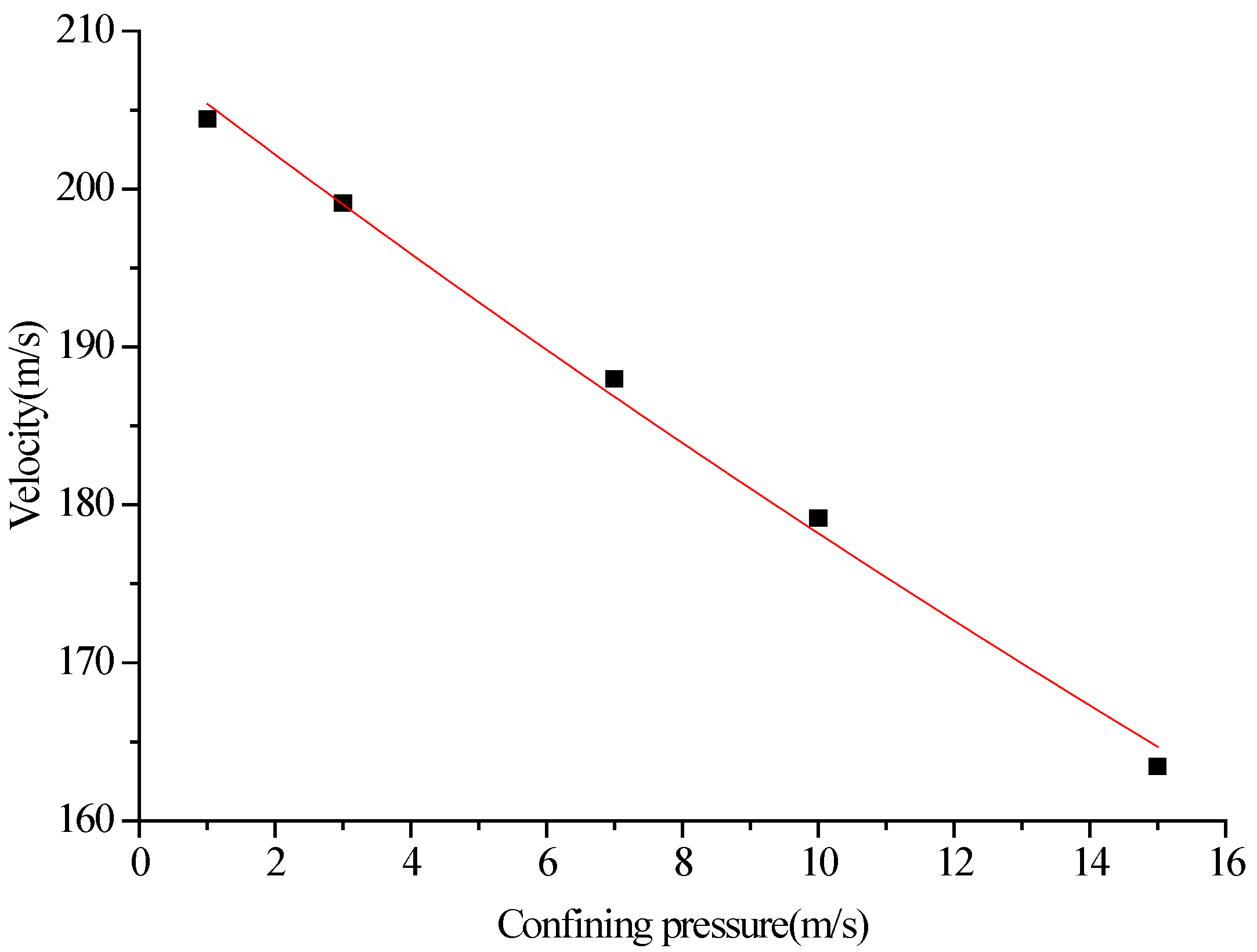
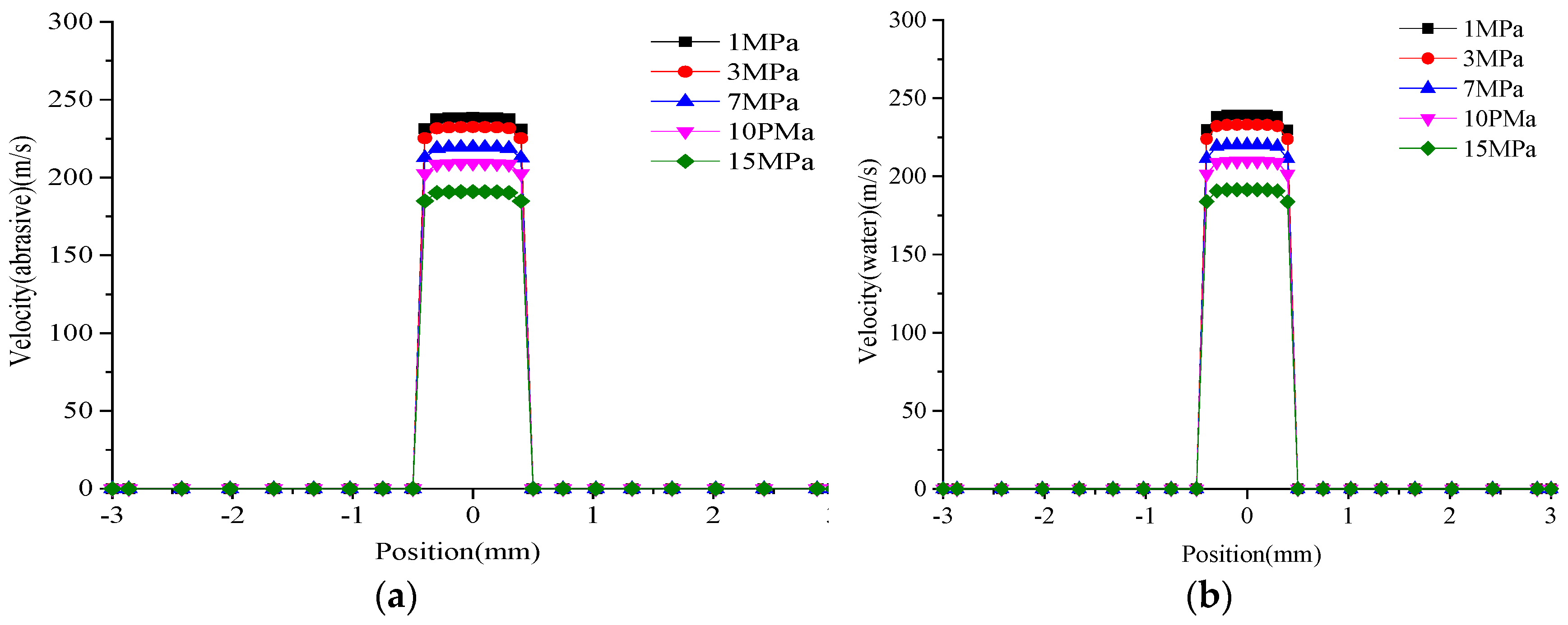
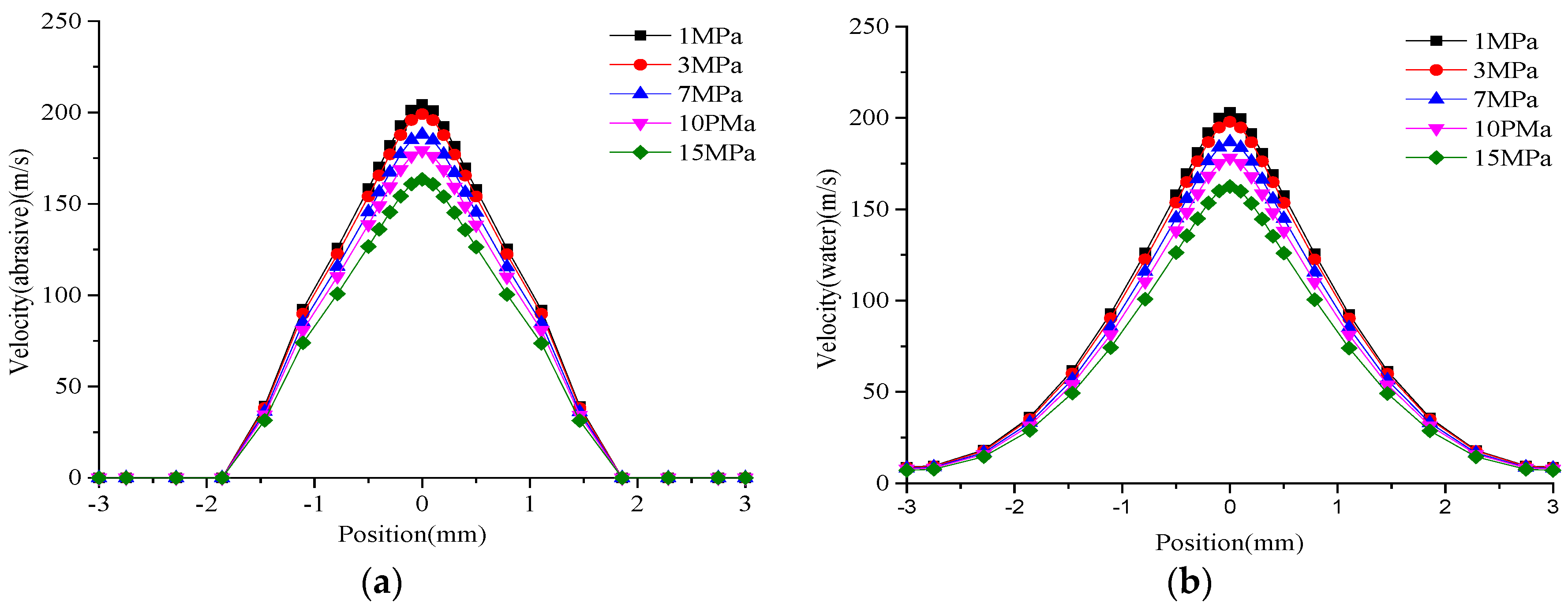
3.2. The Influence of Confining Pressure on the Jet Flow Field

The influence of different confining pressure on the distribution was considered when the abrasive concentration was 10%, the inlet pressure was 40 MPa, and the particle size was 0.2 mm. The numerical simulation was adopted to simulate the jet flow field when the confining pressure was 1 MPa, 3 MPa, 7 MPa, 10 MPa and 15 MPa, respectively.

(1)

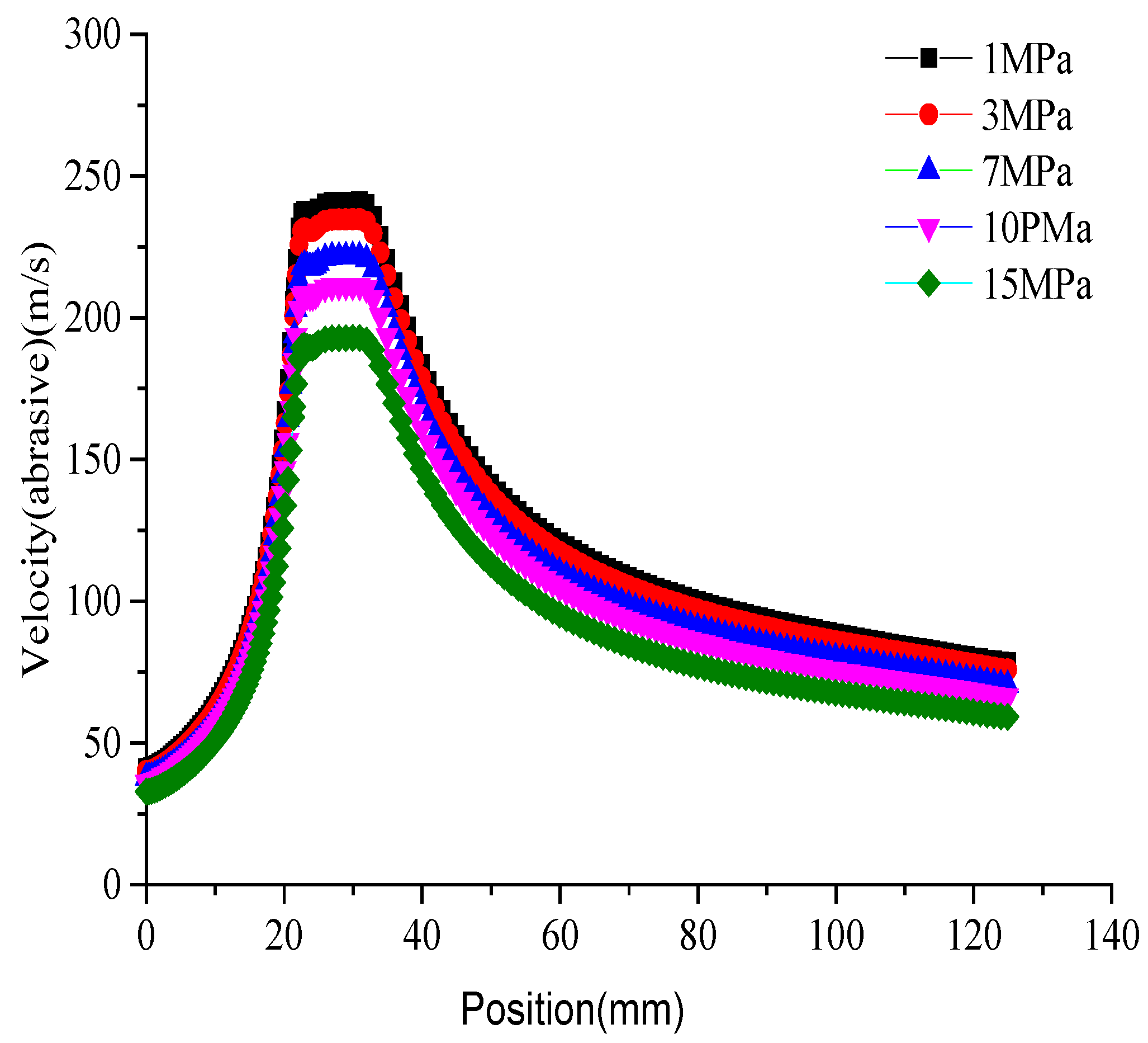
Axial velocity distribution

Figure 8 shows the influence of confining pressure on the axial velocity distribution of the abrasive. As can be seen from the figure, the confining pressure has a certain effect on the axial velocity of the abrasive, and the axial velocity at the same range decreases with the increase of the confining pressure. When the confining pressure is 1MPa, the axial velocity of the abrasive is the largest.

(2)

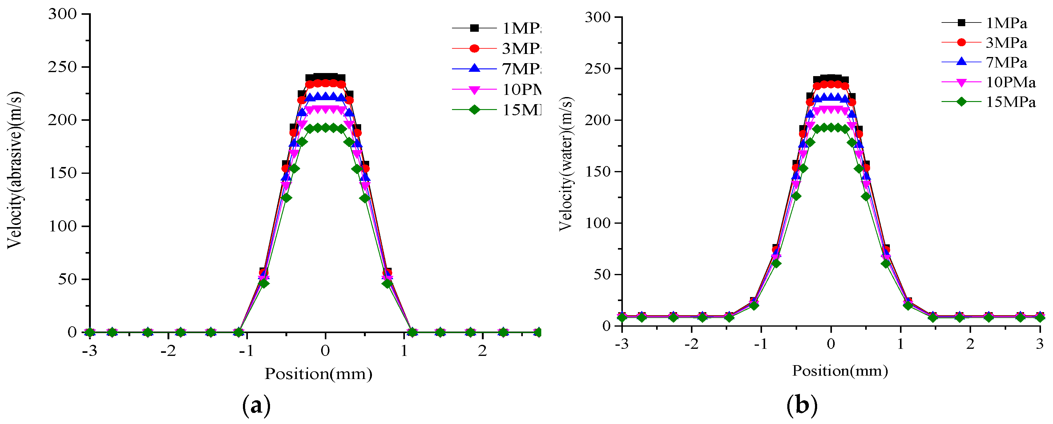
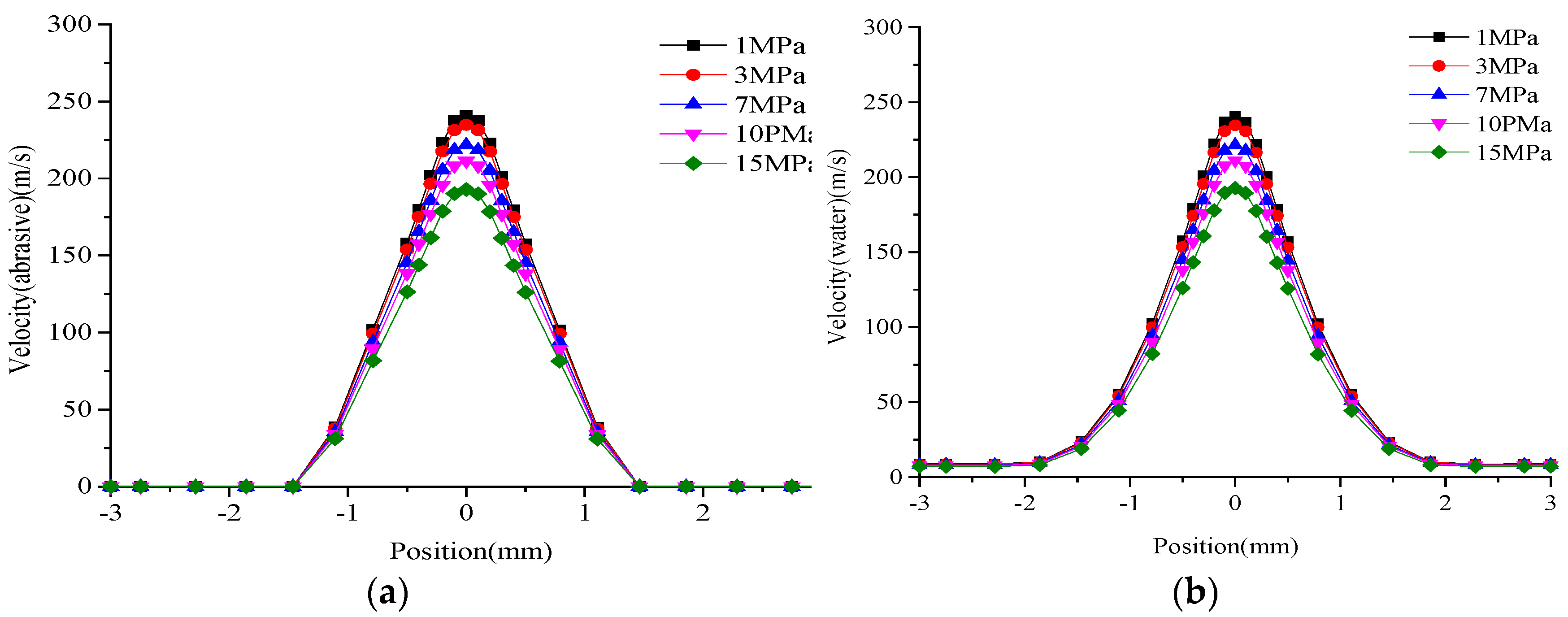
Radial velocity distribution

Figure 9 is the influence of confining pressure on the distribution of the nozzle’s cross section velocity. As can be seen in the figure, the confining pressure has an obvious influence on the radial velocity of the nozzle’s cross section. The radial velocity of the jet at the nozzle exit decreases with the increase in confining pressure, while the velocity difference increases.

Figure 10 is the influence of confining pressure on the distribution of the cross section velocity 3 mm from the nozzle. Figure 11 is the influence of confining pressure on the distribution of the cross section velocity 6 mm from the nozzle. Figure 12 is the influence of confining pressure on the distribution of the cross section velocity 12 mm from the nozzle. As can be seen in the figures, the confining pressure has a certain effect on the axial velocity distribution of different cross sections. At the same radial distance from the same cross section, the jet velocity decreases with the increase in confining pressure.

As can be seen in

Table 2. The influence of confining pressure on the axis velocity of the abrasive.

Confining Pressure (MPa)	The Axis Velocity of the Abrasive (m/s)
	Nozzle Exit	3 mm from the Nozzle Exit	6 mm from the Nozzle Exit	12 mm from the Nozzle Exit
1	238.629	240.933	241.053	204.431
3	232.415	234.659	234.776	199.088
7	219.458	221.578	221.684	187.957
10	209.215	211.237	211.335	179.156
15	190.924	192.771	192.854	163.446

, when the confining pressure decreases from 15 MPa to 10 MPa, the axial velocity of the abrasive will increase by 18.291 m/s. During this process, when the confining pressure decreases by 1 MPa every time, the axial velocity of the abrasive will increase by 3.6582 m/s. When the confining pressure is reduced from 10 MPa to 7 MPa, the axial velocity of the abrasive will increase by 3.414 m/s. And when the confining pressure is reduced from 3MPa to 1MPa, the axial velocity will increase by 3.107 m/s. It can be seen that with the decrease in the abrasive confining pressure, the axial velocity of the nozzle exit increases more and more slowly, as well as the axial velocity in other places. With the increase in the confining pressure, the axial velocity of the abrasive at the same position is increasing continuously.

Figure 13 is the fitting curve of the confining pressure and axial velocity of the abrasive nozzle outlet. As can be seen from the figure, the relationship of the two conforms to the exponential function. And the fitting precision R² = 0.99422. Therefore, the general expression of the relationship between the confining pressure and the axial velocity of the nozzle outlet is:

$$y=243.54017e^{-0.01573x}$$

(20)

Therefore, an abrasive speed of the nozzle exit at any confining pressure can be calculated with the expression. As can be seen from the graph, the axial velocity of the nozzle outlet is decreasing with the increase in confining pressure in the range of 1 MPa~15 MPa.

Figure 14 is the curve fitting the confining pressure and the abrasive axis velocity 3 mm from the nozzle exit. As can be seen from the figure, the relationship of the two conforms to the exponential function, and the fitting precision of R² = 0.99423. Therefore, the general expression of the relationship between the confining pressure and the axial velocity 3mm from the nozzle outlet is:

$$y=245.89086e^{-0.01573x}$$

(21)

Therefore, an abrasive axis velocity 3 mm from the nozzle exit at any confining pressure can be calculated with the expression. As can be seen from the graph, the larger the confining pressure of abrasive axis velocity at the same place, the smaller the velocity.

Figure 15 is the curve fitting of confining pressure and abrasive axis velocity 6 mm from the nozzle exit. As can be seen from the figure, the relationship of the two conforms to the exponential function, and the fitting precision of R² = 0.99422. Therefore, the general expression of the relationship between the confining pressure and the axial velocity 6 mm from the nozzle outlet is:

$$y=246.01594e^{-0.01573x}$$

(22)

Therefore, an abrasive axis velocity 6 mm from the nozzle exit at any confining pressure can be calculated with the expression. As can be seen in the graph, the axial velocity 6 mm from the nozzle outlet increases with the decrease in confining pressure in the range of 1 MPa~15 MPa constantly.

Figure 16 is the curve fitting of the confining pressure and abrasive axis velocity 12 mm from the nozzle exit. As can be seen from the figure, the relationship of the two conforms to the exponential function, and the fitting precision of R² = 0.99423. Therefore, the general expression of the relationship between the confining pressure and the axial velocity 12 mm from the nozzle outlet is:

$$y=208.65008e^{-0.01578x}$$

(23)

Therefore, an abrasive axis velocity 12 mm from the nozzle exit at any confining pressure can be calculated with the expression. As can be seen in the graph, the smaller the confining pressure, the larger the velocity in the range of 1 MPa~15M Pa.

By comparing the relationship between different confining pressures and the axial velocity of the different distances from the nozzle exit, it is known that the relationship between them is in line with the exponential function $y=a{e}^{bx}$. The confining pressure and the axial velocity 0 mm, 3 mm, 6 mm, 12 mm from the nozzle exit respectively fit b = −0.01573, b = −0.01573, b = −0.01573, b = −0.01578 in the function. Therefore, we can see that b is approximately −0.01573 in the function relationship between the confining pressure and the axial velocity of different distances. It can then be concluded that the relationship between them conforms to the exponential function $y=a{e}^{-0.01573x}$, where a is related to the distance from the nozzle exit.

4. Conclusions

(1)

In the convergence section, because of the geometrical structure, the velocity of the jet is increasing and the pressure energy of the abrasive is gradually converted into kinetic energy. After the ejection of the abrasive, the speed increases at the beginning and the maximum speed is 6 mm from the nozzle exit. After the speed reaches the maximum, it will decrease constantly because of the water resistance of the surrounding water zone. The entire jet section develops into a form of axial high speed, which then decreases along the radial direction at the nozzle exit.

(2)

The simulation calculation of two-phase flow with different sizes of abrasive particles has been carried out. As can be seen in the simulation results, the abrasive particle size has little effect on the velocity field outside the nozzle. The greater the particle size, the greater the kinetic energy and the greater the cutting ability. However, the diameter of the nozzle outlet is certain, so the abrasive particle size cannot be too large.

(3)

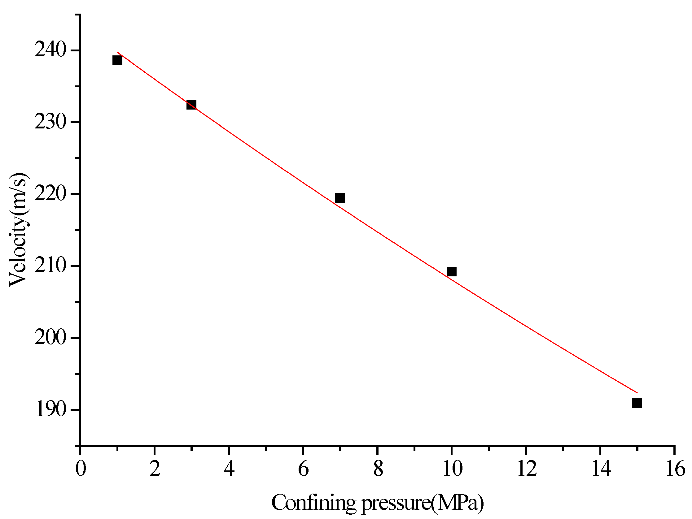
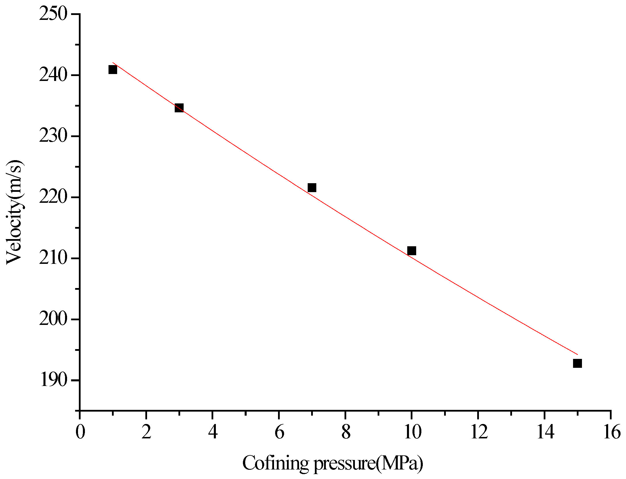
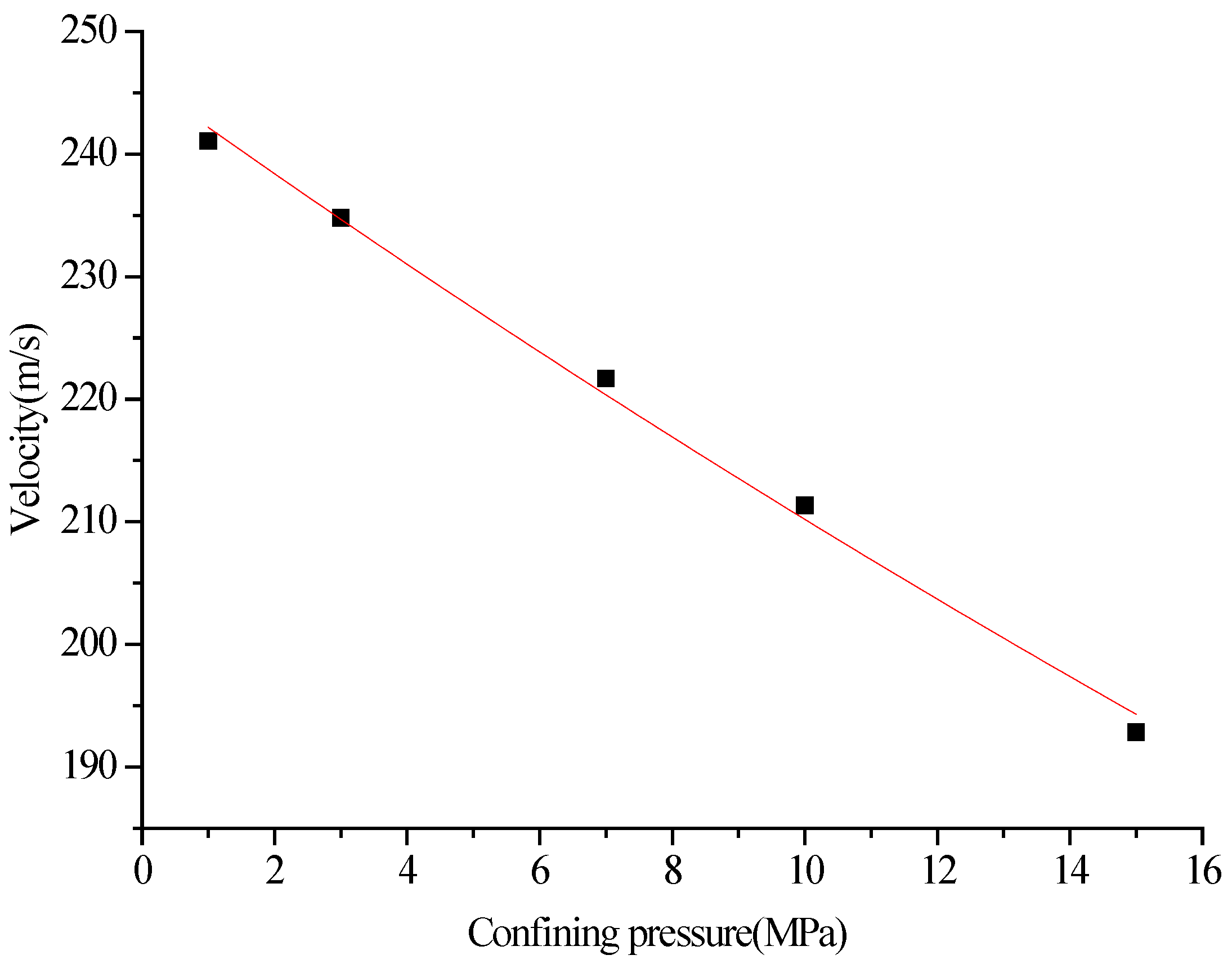
The simulation calculation of two-phase flow with different confining pressures has been carried out. As can be seen in the simulation results, the jet velocity decreases constantly with the increase in confining pressure in the same place, and the relationship between the confining pressure and the axial velocity of the nozzle exit at different distances from the nozzle is in accordance with the exponential function.

References

- Cui, M.; Li, C. Basic research on premixed abrasive water jet nozzle. China Saf. Sci. J. 1995, 5, 138–145. (In Chinese) [Google Scholar]
- Li, B.; Guo, C. Study on acceleration mechanism of abrasive particles of DIA jet in safe cutting. China Saf. Sci. J. 2005, 15, 52–55. (In Chinese) [Google Scholar]
- Li, X.; Sun, J.; Wang, J. Feasibility testing and investigation on a new technology for hard rock tunneling with a collimated abrasive water jet. Chin. J. Rock Mech. Eng. 2001, 20, 61–64. [Google Scholar] [CrossRef]
- Li, B. Development of safe cutting device in inflammable and explosive place. Fluid Mach. 2005, 33, 42–44. [Google Scholar]
- Lin, B.; Lv, Y.; Li, B. High-pressure abrasive hydraulic cutting seam technology and its application in outbursts prevention. J. China Coal Soc. 2007, 32, 959–963. [Google Scholar]
- Li, X.; Lu, Y.; Zhao, Y. Study on improving the permeability of soft coal seam with high pressure pulsed water jet. J. China Coal Soc. 2008, 33, 1386–1390. [Google Scholar]
- Liu, L. Simulation and Experimental Validation on the Flow Field Inside and Outside the Nozzle of Non-Submersed Precision Micro Abrasive Waterjet; Shandong University: Jinan, China, 2008. [Google Scholar]
- W, D.; Wu, Y.; Luo, W.; Xiang, Y. Study of flow field on cutting with high pressure water jet. J. Wuhan Univ. Sci. Eng. 2005, 18, 15–18. [Google Scholar]
- Wang, M.; Wang, R. Numerical simulation on fluid-particle two-phase jet flow field in nozzle. J. Univ. Pet. China 2005, 29, 46–49. [Google Scholar]
- Chen, C.; Nie, S.; Wu, Z.; Li, Z. A study of high pressure water jet characteristics by CFD simulation. Mach. Tool Hydraul. 2006, 2, 103–105. [Google Scholar]
- Qu, Y.; Chen, S.; Wang, X.; Teng, S. Discussion of the numerical simulation of ax-symmetric jet with different turbulent model. J. Eng. Thermophys. 2008, 6, 957–959. [Google Scholar]
- Gao, J.; Hu, S.; Ning, Y. The study of numerical simulation and flow characteristics of submerged abrasive jet based on CFD. China Mech. Eng. 2003, 14, 1188–1191. [Google Scholar]
- Dong, X. Numerical simulation study of the nozzle inside-flow of premixed abrasive water jet. Mach. Design Res. 2005, 21, 87–91. (In Chinese) [Google Scholar]
- Hou, R.G.; Huang, C.Z.; Wang, J.; Lu, X.Y.; Feng, Y.X. Simulation of solid-liquid two-phase flow inside and outside the abrasive water jet nozzle. Key Eng. Mater. 2007, 339, 453–457. [Google Scholar] [CrossRef]
- Su, M.; Huang, S. Foundation of Computational Fluid Dynamics; Tsinghua University Press: Beijing, China, 1997. (In Chinese) [Google Scholar]
- Hu, G.; Yu, T.; Liu, X. The numerical simulation of two phase flow about the liquid and solid in nozzle of DIA jet. Mechatronics 2005, 16, 20–23. (In Chinese) [Google Scholar]
- Saxena, A.; Paul, S. Numerical modelling of kerf geometry in abrasive water jet machining. Int. J. Abras. Technol. 2007, 1, 208–230. [Google Scholar] [CrossRef]
- Nie, B.; Meng, J.; Ji, Z. Numerical simulation research of liquid-solid two-phase flow in abrasive water jet nozzle. J. Beijing Inst. Technol. 2009, 18, 157–161. [Google Scholar]
- Meng, J.; Nie, B.; Ma, Y. Study on abrasive mixing chamber of pre-mixed water jet. Gazi Univ. J. Sci. 2015, 28, 425–431. [Google Scholar]
- Liu, G.; Wang, K.; Chen, X. Numerical simulation of internal flow field for post-mixed abrasive water jet descaling nozzle. Gongcheng Kexue Xuebao/Chin. J. Eng. 2015, 37, 29–34. [Google Scholar] [CrossRef]