An Improved Bald Eagle Search Algorithm for Parameter Estimation of Different Photovoltaic Models

Abstract

Clean energy resources have become a worldwide concern, especially photovoltaic (PV) energy. Solar cell modeling is considered one of the most important issues in this field. In this article, an improvement for the search steps of the bald eagle search algorithm is proposed. The improved bald eagle search (IBES) was applied to estimate more accurate PV model parameters. The IBES algorithm was applied for conventional single, double, and triple PV models, in addition to modified single, double, and triple PV models. The IBES was evaluated by comparing its results with the original BES through 15 benchmark functions. For a more comprehensive analysis, two evaluation tasks were performed. In the first task, the IBES results were compared with the original BES for parameter estimation of original and modified tribe diode models. In the second task, the IBES results were compared with different recent algorithms for parameter estimation of original and modified single and double diode models. All tasks were performed using the real data for a commercial silicon solar cell (R.T.C. France). From the results, it can be concluded that the results of the modified models were more accurate than the conventional PV models, and the IBES behavior was better than the original BES and other compared algorithms.

1. Introduction

The high demand for clean energy is increasing the development cycles of PV systems. The solar cell is considered the basic element in PV systems. The rapid development in photovoltaic energy has a great effect on perceptions of the importance of solar cell modeling. The modeling of PV systems plays a vital role in the design phase due to the availability of simulation and testing for the PV system before the construction phase. The history of PV modeling began in the last decade [1].

There are different types of models described in the literature. These models rely on the diodes as their main components, as well as some resistors to represent the properties of the photovoltaic cells. However, the main challenge facing these models is obtaining the best values for individual parameters, such as impedance, diode ideal factors, and saturation currents, in order to enable successful modeling [2]. SDMs are considered the basic model and have one diode in the model, but DDMs and TDMs have two and three diodes, respectively. The development of a more detailed model would be more suitable for representing a wide range of PV systems at different operating conditions, like low irradiance conditions [3]. Moreover, the detailed models are more capable of representing different physical PV properties, such as the effect of grain boundaries, the leakage current, and the recombination current in multi-crystalline silicon solar cells [4]. For the previous reasons, many modifications of the models have been proposed in the literature. The authors of [3] proposed a modified DDM; the modification is based on adding a resistance in series with the second diode to represent the effect of grain boundary regions. The MDDM was selected in this study to represent the complex multi-crystalline solar cell due to its advantages in representing the effect of grain boundaries, as discussed in [5]. A modified TDM was therein proposed and compared with the MDDM. The authors concluded that the obtained results from the MTDM were better than those of the MDDM, and that this indicates that MTDMs are more accurate than MDDMs. Three modified models were proposed in [6], the MSD, MDDM, and MTDM. From their results, the authors concluded that the three modified models were more reliable and accurate than the traditional three PV models. In all the previous studies reviewed, the researchers used different optimization techniques to estimate the parameters of the PV models. The selection of a suitable algorithm for this task is a challenge due to the complexity of the detailed PV models [7,8,9,10,11,12]. This challenge has led many researchers to propose enhancements to original optimization algorithms to improve their performance with this problem and other similar complex problems [13,14,15,16,17]. The bald eagle search (BES) algorithm a recent meta-heuristic algorithm proposed in [18]. BES, like GWO and HHO, is inspired by animal hunting behavior. The BES algorithm is inspired by bald eagles’ searching and hunting behavior in relation to its food (fish and so on). The behavior of population-based algorithms differs from one objective function to another and depends on different factors, like the initial population and a proper search range [19,20,21,22,23]. In this work, an improvement to the BES algorithm, called the IBES algorithm, is proposed. The IBES is based on changing the learning parameter that controls the change in position in each iteration from a constant parameter to a variable parameter as its value changes in each iteration. The IBES changes the value of this parameter based on a decay equation to enhance its exploration and exploitation. The IBES was tested on 23 benchmark functions and was used to estimate the parameters of different complex detailed PV models.

The main contributions of this work can be briefly summarized as follows:

-

A detailed description of the three main conventional PV models (SDM, DDM, and TDM) is provided;

-

A detailed description of the three modified PV models (MSDM, MDDM, and MTDM) is provided;

-

An improved algorithm (IBES) is proposed and detailed discussion about testing the behavior of the improved algorithm on 23 benchmark functions is provided;

-

The improved algorithm and the original BES are compared through their application to the estimation of the parameters of the modified triple diode model (MTDM) and original triple diode model (TDM);

-

For more comprehensive results, the performance of IBES and other recent algorithms is compared for the estimation of the parameters of the SDM, MSDM, DDM, and MDDM;

-

In all the applications, the real data from an RTC furnace solar cell were used as a dataset for the objective function;

-

The performance of the IBES and other compared algorithms is evaluated through statistical analysis.

The rest of this paper is arranged as follows. Section 2 presents the PV modeling analysis. Section 3 presents the proposed IBES. The simulation results are discussed in Section 4. Section 5 summarizes the conclusion of the work.

2. PV Mathematical Model

In this section, the mathematical models of the three PV models, the SDM, DDM, and TDM, are discussed in detail through the equations of each model. A modification to the previous models, based on adding new series resistance (Rsm) to express the losses in different regions, is also discussed [5,6]. The three modified models are the MSDM, MDDM, and MTDM.

2.1. SDM and MSDM

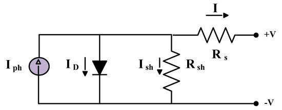
The SDM is considered the most basic and simple PV model when compared with other models. Figure 1 presents the equivalent circuit of the SDM. Based on Figure 1, the PV output current can be described by Equations (1) and (2). The five main parameters (R_s, R_sh, I_ph, I_s1, and η) can be described as X = [X₁, X₂, X₃, X₄, X₅]. The problem objective function is described in Equation (3):

$$I=I_{ph}-I_D-I_{sh}$$

(1)

$$I_{}=I_{ph}-I_{s1}\left[\exp (\frac{q(V_{}+R_s\ast I)}{\eta \ast K\ast T})-1\right]-\frac{(V+R_s\ast I_{})}{R_{sh}}$$

(2)

$$f_{SD}(V,I,X)=I-X_3+X_4\left[\exp (\frac{q(V+R_s\ast I)}{X_5\ast K\ast T})-1\right]+\frac{(V+X_1\ast I)}{X_2}$$

(3)

Figure 1. The SDM.

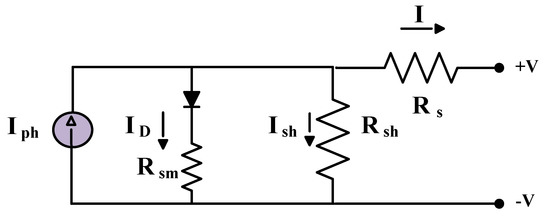
Figure 2 presents the equivalent circuit of the MSDM. The main difference between the MSDM and SDM is a resistance (R_sm) connected in series with the diode to represent the losses in the quasi-neutral region. Based on Figure 2, the PV output current can be described as in Equation (4). The six main parameters (R_s, R_sh, I_ph, I_s1, η, and R_sm) can be described as X = [X₁, X₂, X₃, X₄, X₅, X₆]. The problem objective function is described in Equation (5):

$$I_{}=I_{ph}-I_{s1}\left[\exp (\frac{q(V_{}+R_s\ast I-R_{sm}\ast I_D)}{\eta \ast K\ast T})-1\right]-\frac{(V+R_s\ast I_{})}{R_{sh}}$$

(4)

$$f_{SD}(V,I,X)=I-X_3+X_4\left[\exp (\frac{q(V+X_1\ast I-X_6\ast I_D)}{X_5\ast K\ast T})-1\right]+\frac{(V+X_1\ast I)}{X_2}$$

(5)

Figure 2. The MSDM.

2.2. DDM and MDDM

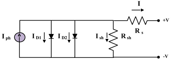
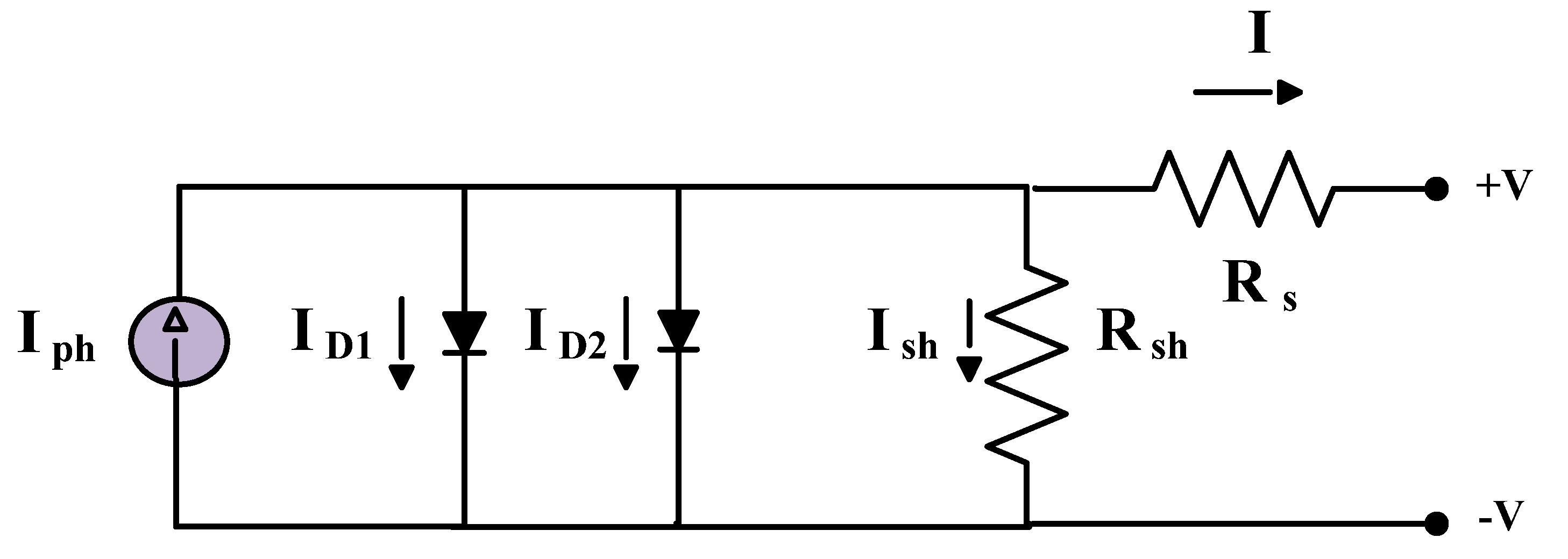
The DDM consists of two diodes that represent the recombination current of a solar cell. Figure 3 presents the equivalent circuit of the DDM. Based on Figure 3, the PV output current can be described by Equations (6) and (7). The seven main parameters (R_s, R_sh, I_ph, I_s1, I_s2, η₁, and η₂) can be described as X = [X₁, X₂, X₃, X₄, X₅, X₆, X₇]. The problem objective function is described in Equation (8):

$$I=I_{ph}-I_{D1}-I_{D2}-I_{sh}$$

(6)

$$I=I_{ph}-I_{s1}\left[\exp (\frac{q(V+R_s\ast I)}{{\eta }_1\ast K\ast T})-1\right]-I_{s2}\left[\exp (\frac{q(V+R_s\ast I)}{{\eta }_2\ast K\ast T})-1\right]-\frac{(V+R_s\ast I)}{R_{sh}}$$

(7)

$$f_{DD}(V,I,X)=I-X_3+X_4\left[\exp (\frac{q(V+X_1\ast I)}{X_6\ast K\ast T})-1\right]+X_5\left[\exp (\frac{q(V+X_1\ast I)}{X_7\ast K\ast T})-1\right]+\frac{(V+X_1\ast I)}{X_2}$$

(8)

Figure 3. The DDM.

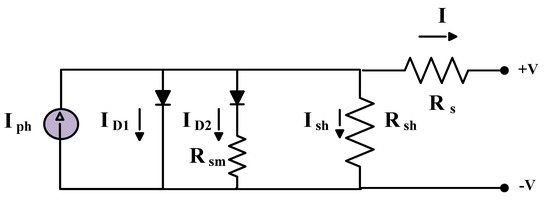
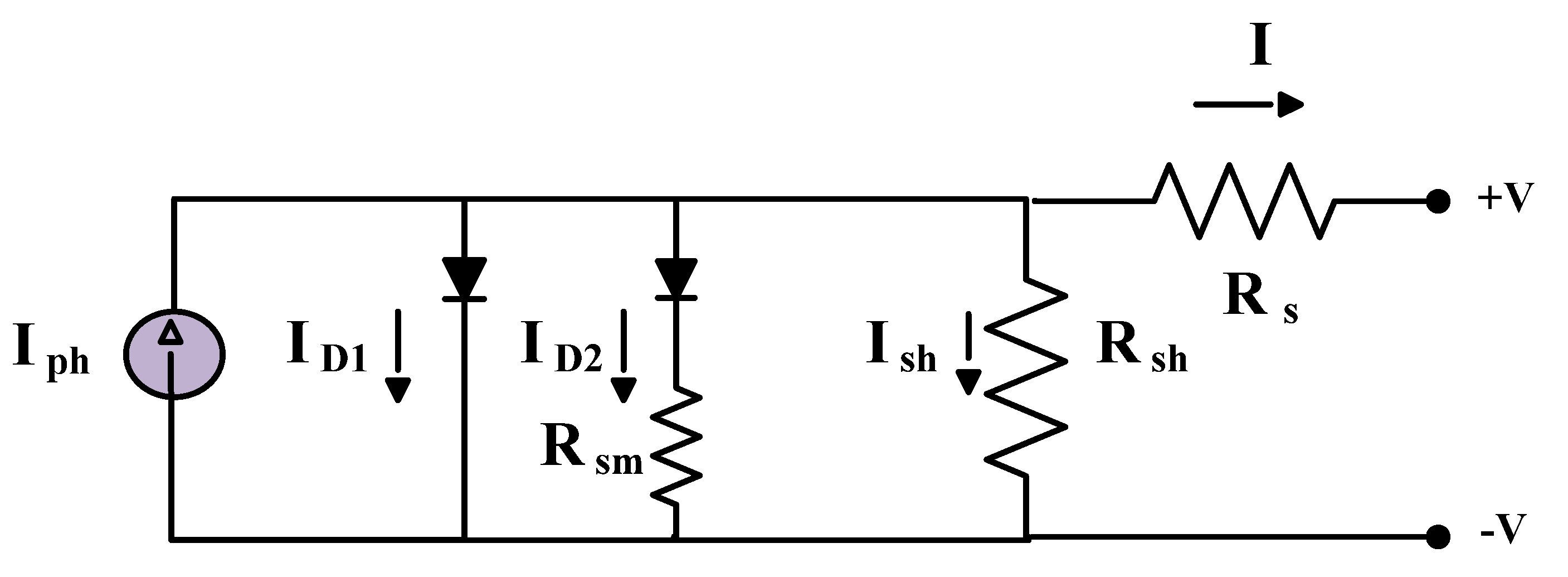
The MDDM is the same as the DDM, utilizing series resistance (R_sm) with diode 2 to represent the losses in the space charge region. Figure 4 presents the equivalent circuit of the MDDM. Based on Figure 4, the PV output current can be described by Equation (9). The eight main parameters (R_s, R_sh, I_ph, I_s1, I_s2, η₁, η₂, and R_sm) can be described as X = [X₁, X₂, X₃, X₄, X₅, X₆, X₇, X₈]. The problem objective function is described in Equation (10):

$$I=I_{ph}-I_{s1}\left[\exp (\frac{q(V+R_s\ast I)}{{\eta }_1\ast K\ast T})-1\right]-I_{s2}\left[\exp (\frac{q(V+R_s\ast I-R_{sm}\ast I_{D2})}{{\eta }_2\ast K\ast T})-1\right]-\frac{(V+R_s\ast I)}{R_{sh}}$$

(9)

$$f_{DD}(V,I,X)=I-X_3+X_4\left[\exp (\frac{q(V+X_1\ast I)}{X_6\ast K\ast T})-1\right]+X_5\left[\exp (\frac{q(V+X_1\ast I-X_8\ast I_{D2})}{X_7\ast K\ast T})-1\right]+\frac{(V+X_1\ast I)}{X_2}$$

(10)

Figure 4. The MDDM.

2.3. TDM and MTDM

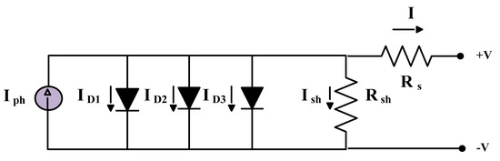
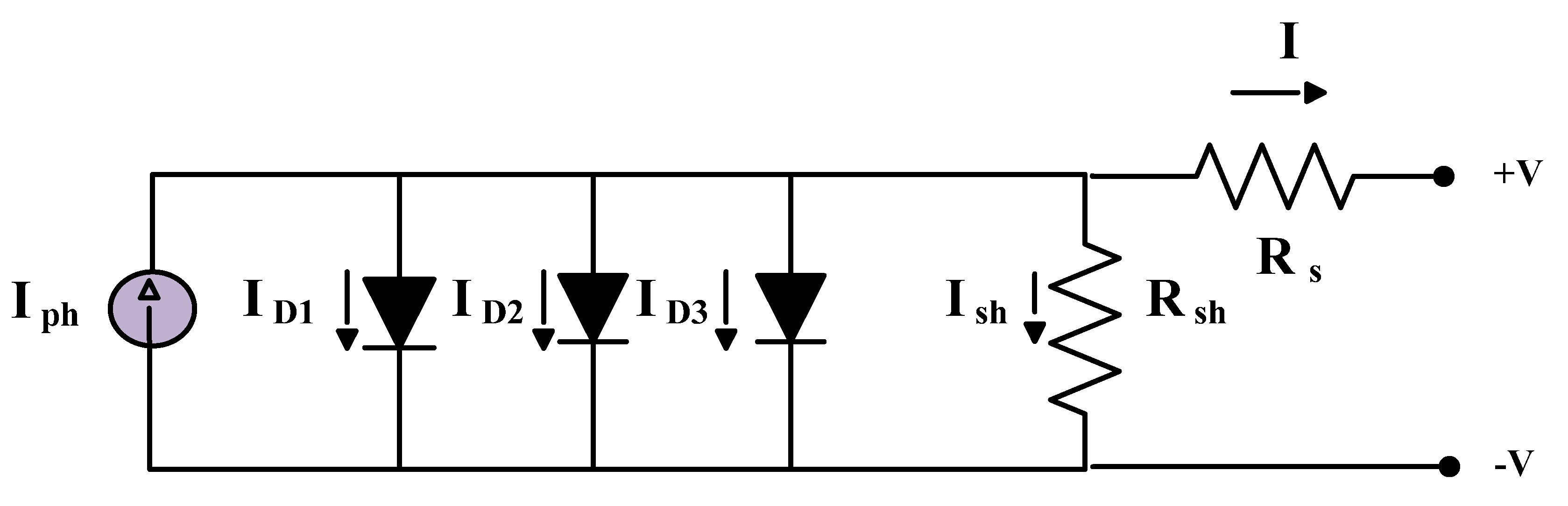
The TDM is based on three diodes, as shown in Figure 5, that represent the effects of grain boundaries and a large leakage current. Based on Figure 5, the PV output current can be described by Equations (11) and (12). The nine main parameters (R_s, R_sh, I_ph, I_s1, I_s2, I_s3, η₁, η₂, and η₃) can be described as X = [X₁, X₂, X₃, X₄, X₅, X₆, X₇, X₈, X₉]. The problem objective function is described in Equation (13):

$$I=I_{ph}-I_{D1}-I_{D2}-I_{D3}-I_{sh}$$

(11)

$$I=I_{ph}-I_{s1}\left[\exp (\frac{q(V+R_s\ast I)}{{\eta }_1\ast K\ast T})-1\right]-I_{s2}\left[\exp (\frac{q(V+R_s\ast I)}{{\eta }_2\ast K\ast T})-1\right]-I_{s3}\left[\exp (\frac{q(V+R_s\ast I)}{{\eta }_3\ast K\ast T})-1\right]-\frac{(V+R_s\ast I)}{R_{sh}}$$

(12)

$$f_{TD}(V,I,X)=I-X_3+X_4\left[\exp (\frac{q(V+X_1\ast I)}{X_7\ast K\ast T})-1\right]+X_5\left[\exp (\frac{q(V+X_1\ast I)}{X_8\ast K\ast T})-1\right]+X_6\left[\exp (\frac{q(V+X_1\ast I)}{X_9\ast K\ast T})-1\right]+\frac{(V+X_1\ast I)}{X_2}$$

(13)

Figure 5. The TDM.

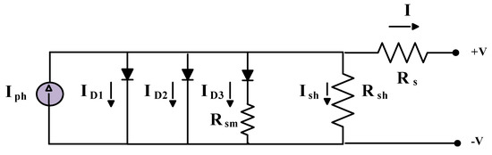
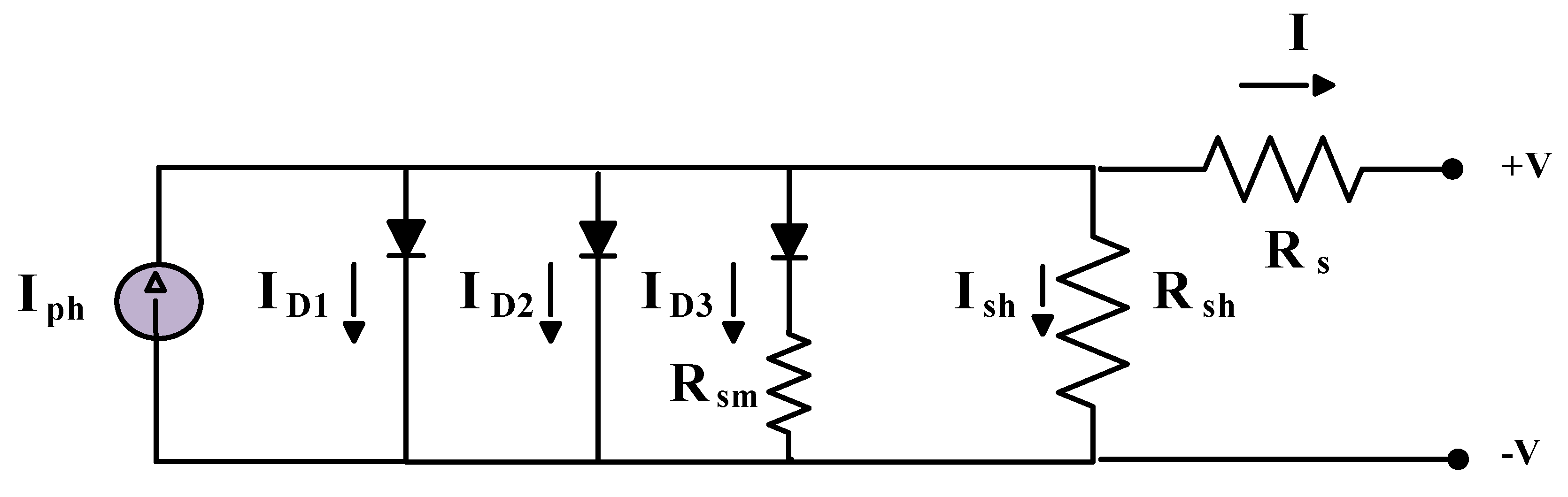
The MTDM is the same as the TDM, utilizing series resistance (R_sm) with the third diode to represent the losses in the defect region, as presented in Figure 6. Based on Figure 6, the PV output current can be described by Equation (14). The ten main parameters (R_s, R_sh, I_ph, I_s1, I_s2, I_s3, η₁, η₂, η₃, and R_sm) can be described as X = [X₁, X₂, X₃, X₄, X₅, X₆, X₇, X₈, X₉, X₁₀]. The problem objective function is described in Equation (15):

$$I=I_{ph}-I_{s1}\left[\exp (\frac{q(V+R_s\ast I)}{{\eta }_1\ast K\ast T})-1\right]-I_{s2}\left[\exp (\frac{q(V+R_s\ast I)}{{\eta }_2\ast K\ast T})-1\right]-I_{s3}\left[\exp (\frac{q(V+R_s\ast I-R_{sm}\ast I_{D3})}{{\eta }_3\ast K\ast T})-1\right]-\frac{(V+R_s\ast I)}{R_{sh}}$$

(14)

$$f_{TD}(V,I,X)=I-X_3+X_4\left[\exp (\frac{q(V+X_1\ast I)}{X_7\ast K\ast T})-1\right]+X_5\left[\exp (\frac{q(V+X_1\ast I)}{X_8\ast K\ast T})-1\right]+X_6\left[\exp (\frac{q(V+X_1\ast I-X_{10}\ast I_{D3})}{X_9\ast K\ast T})-1\right]+\frac{(V+X_1\ast I)}{X_2}$$

(15)

Figure 6. The TDM.

3. Improved Bald Eagle Search Algorithm

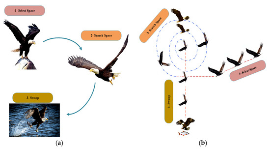
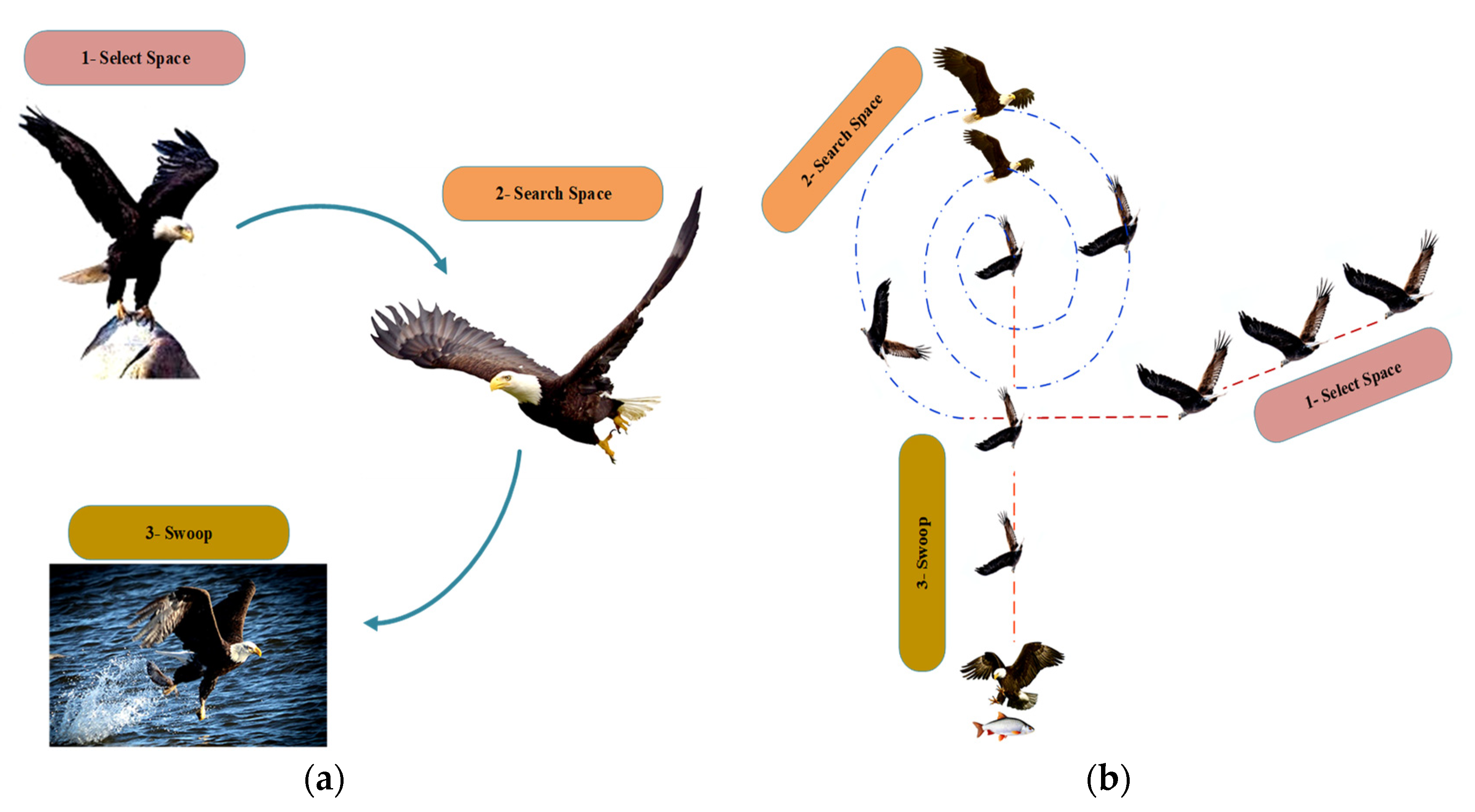
The improved bald eagle search algorithm, based on the original BES, is inspired by bald eagle search behavior during the hunting process. The hunting process can be divided to three sub-processes: selecting the space, searching the space, and, finally, swooping in on the prey (Figure 7).

Figure 7. (a) Behavior of bald eagle during hunting; (b) sequential stages of bald eagle hunting.

-

Selecting the space

In this stage, the blades select the space randomly based on the previous search information (Equation (16)):

$$p_{new, i}=p_{best}+\alpha \times r\left(p_{mean}-p_i\right)$$

(16)

The parameter α for controlling the changes in position can be formulated from the following equation rather than being fixed value, as it is in the original BES algorithm:

$$\alpha =\frac{1.5 · \left(Max\_iter-t+1\right)}{Max\_iter}$$

(17)

This parameter affects the position of the bald eagles and enhances the exploration and exploitation in the IBES technique. r is a random value between 0 and 1. p_new and p_best are the new and current search spaces, respectively. p_mean indicates that these eagles have consumed all the information from the previous points.

-

Search stage

After selecting the search space in the previous step, the eagles start the search for prey in this space by moving in a spiral shape to quicken the search. In this stage, the eagle position is updated based on Equation (18):

$$p_{i, new}=p_i+y\left(i\right)\times \left(p_i-p_{i+1}\right)p_{best}+x\left(i\right)\times r\left(p_i-p_{mean}\right)$$

(18a)

$$x\left(i\right)=\frac{xr\left(i\right)}{max\left(\left|xr\right|\right)},y\left(i\right)=\frac{yr\left(i\right)}{max\left(\left|yr\right|\right)}$$

(18b)

$$xr\left(i\right)=r\left(i\right)\times sin(\theta \left(i\right), yr\left(i\right)=r\left(i\right)\times cos\left(\theta \left(i\right)\right)$$

(18c)

$$\theta \left(i\right)=\alpha \times \pi \times rand$$

(18d)

$$r\left(i\right)=\theta \left(i\right)\times R\times rand$$

(18e)

where α is a parameter that takes a value from 5 to 10 and R is a parameter that takes a value from 0.5 to 2.

-

Swooping stage

In this stage, the eagles start to move from the best search position towards their prey in a swing movement described in Equation (19):

$$P_{i,new}=rand \ast P_{best}+x_1 \left(i\right)\times \left(P_i-c_1 \ast P_{mean}\right)+y_1\left(i\right)\times \left(P_i-C_2 \ast P_{best}\right)$$

(19)

$$x1\left(i\right)=\frac{xr\left(i\right)}{max\left(\left|xr\right|\right)},y1\left(i\right)=\frac{yr\left(i\right)}{max\left(\left|yr\right|\right)}$$

$$xr\left(i\right)=r\left(i\right)\ast sinh\left[\left(\theta \left(i\right)\right], yr\left(i\right)=r\left(i\right)\times cosh\right[\left(\theta \left(i\right)\right)]$$

$$\theta \left(i\right)=\alpha \times \pi \times rand\hspace{1em}r\left(i\right)=\theta \left(i\right)$$

where c1, c2 ϵ [1, 2].

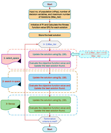
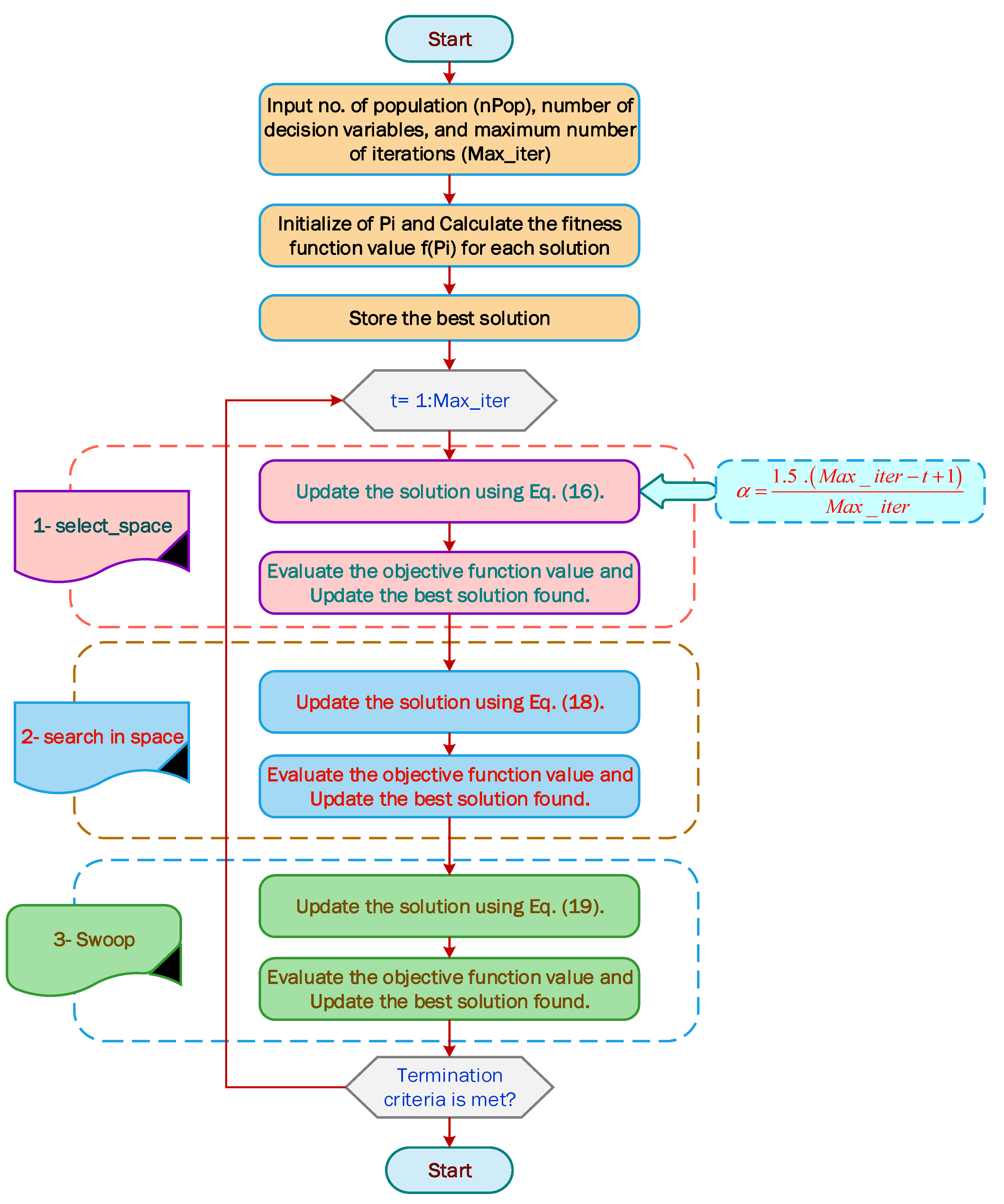
A flowchart describing the entire IBES algorithm is presented in Figure 8.

Figure 8. Flowchart for the IBES algorithm.

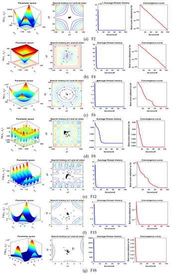
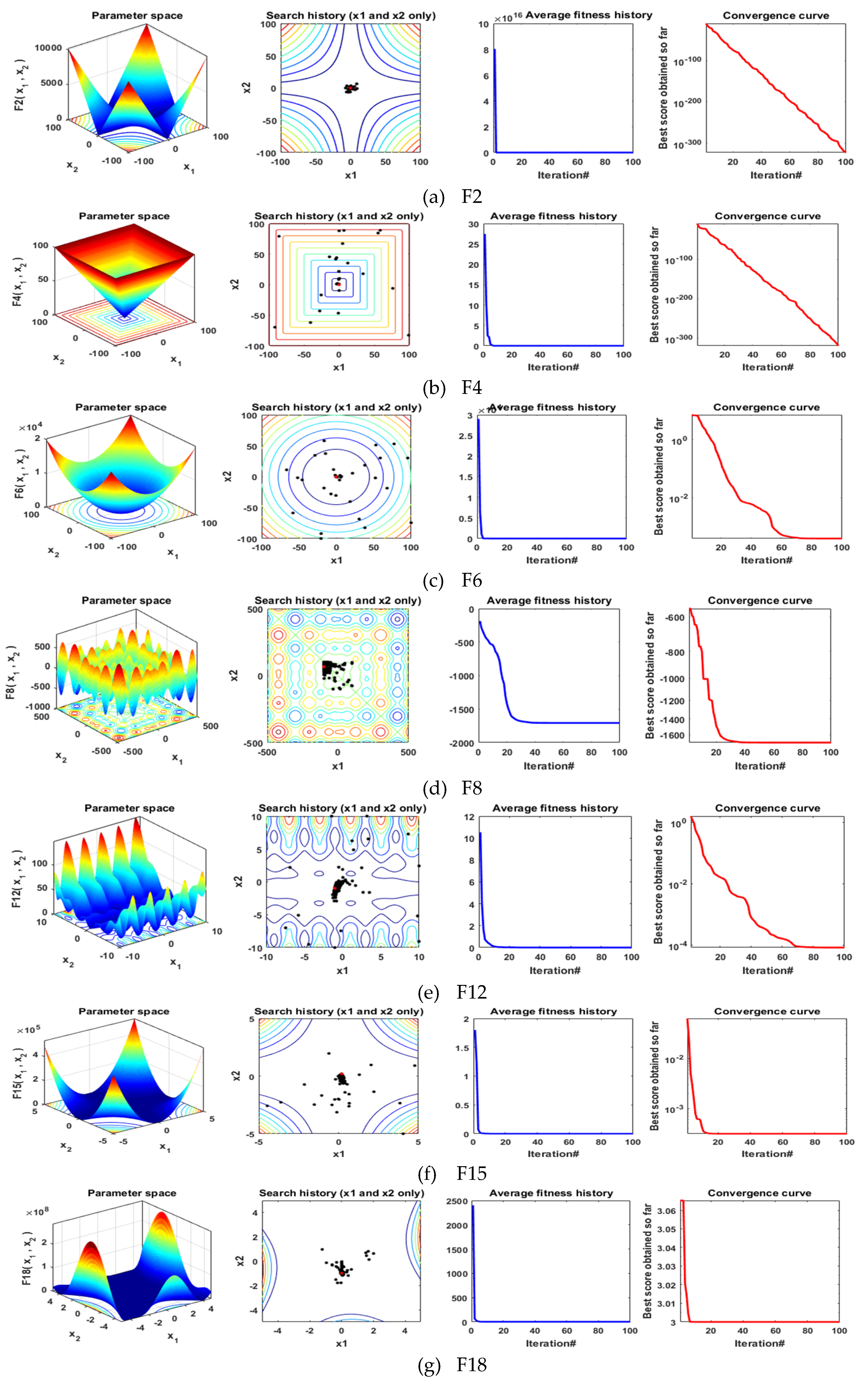
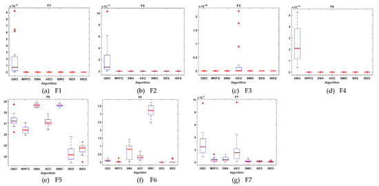
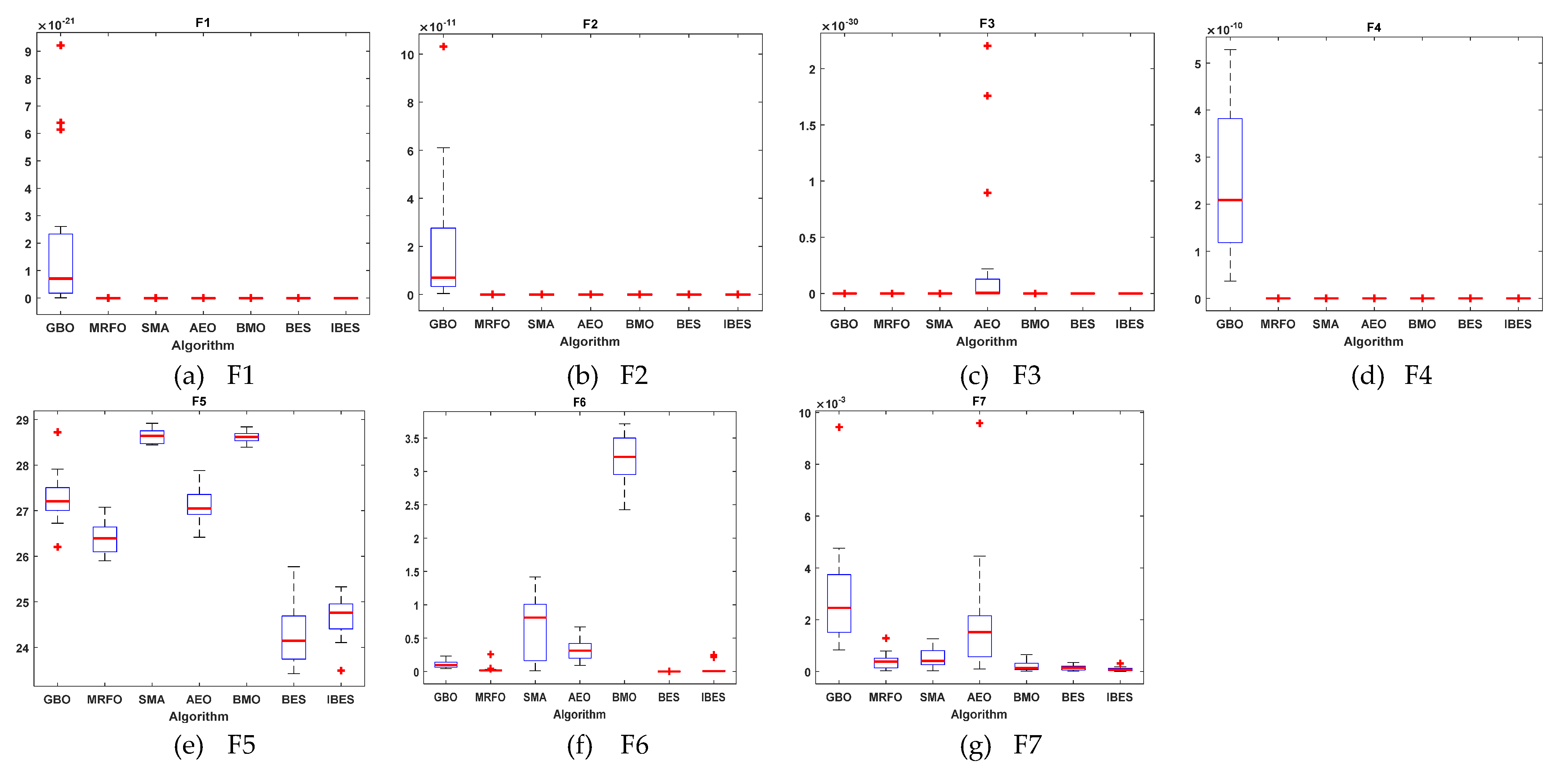
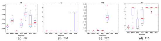
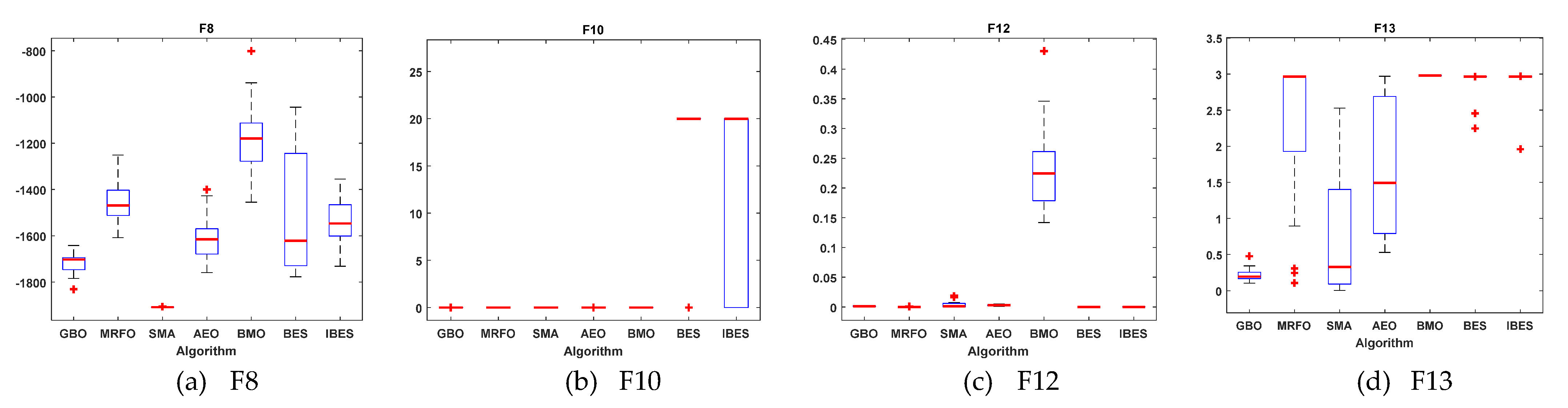
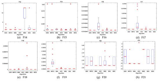
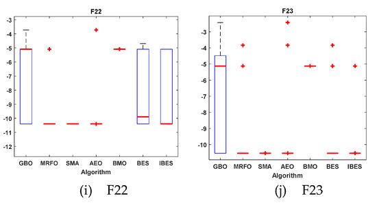
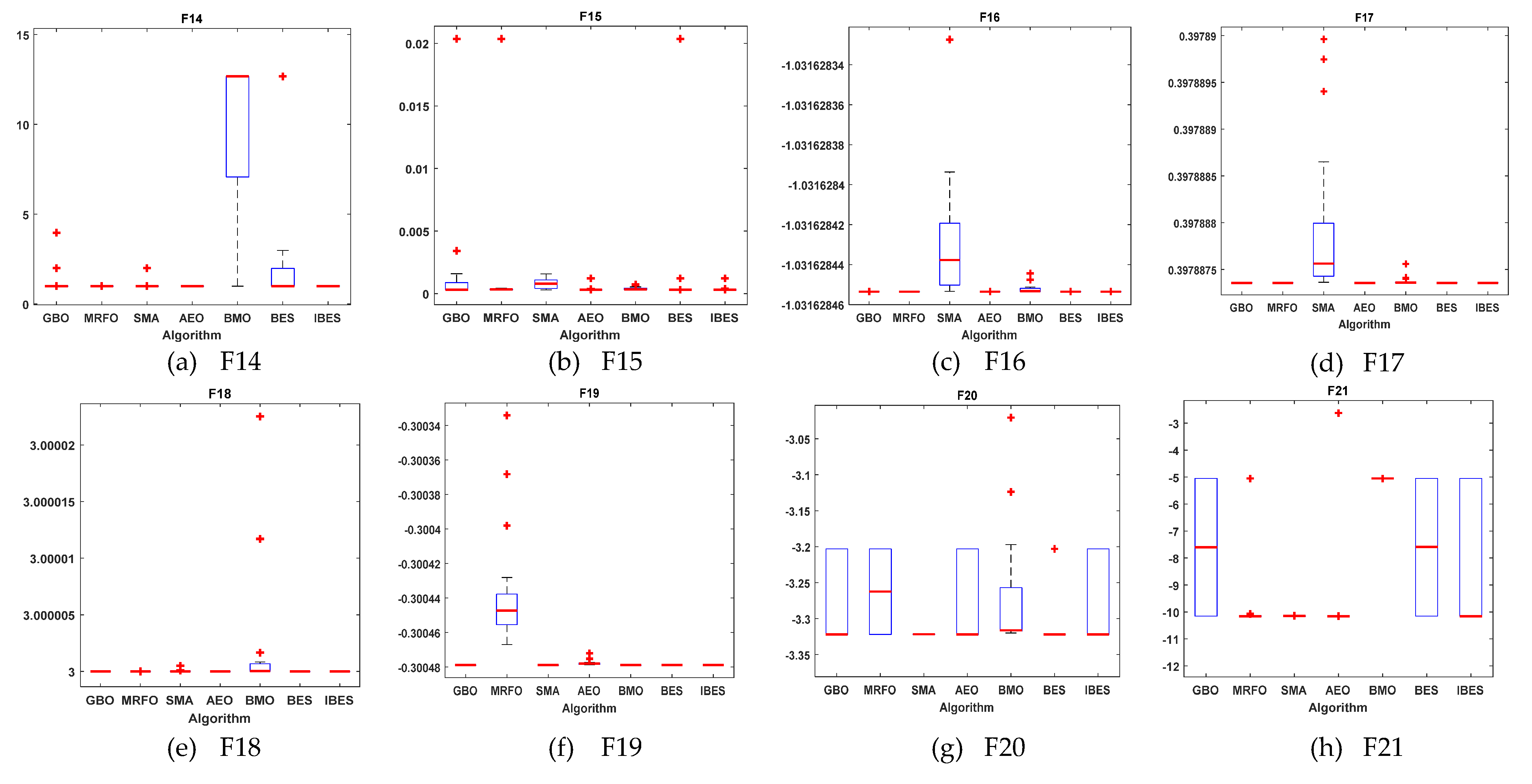
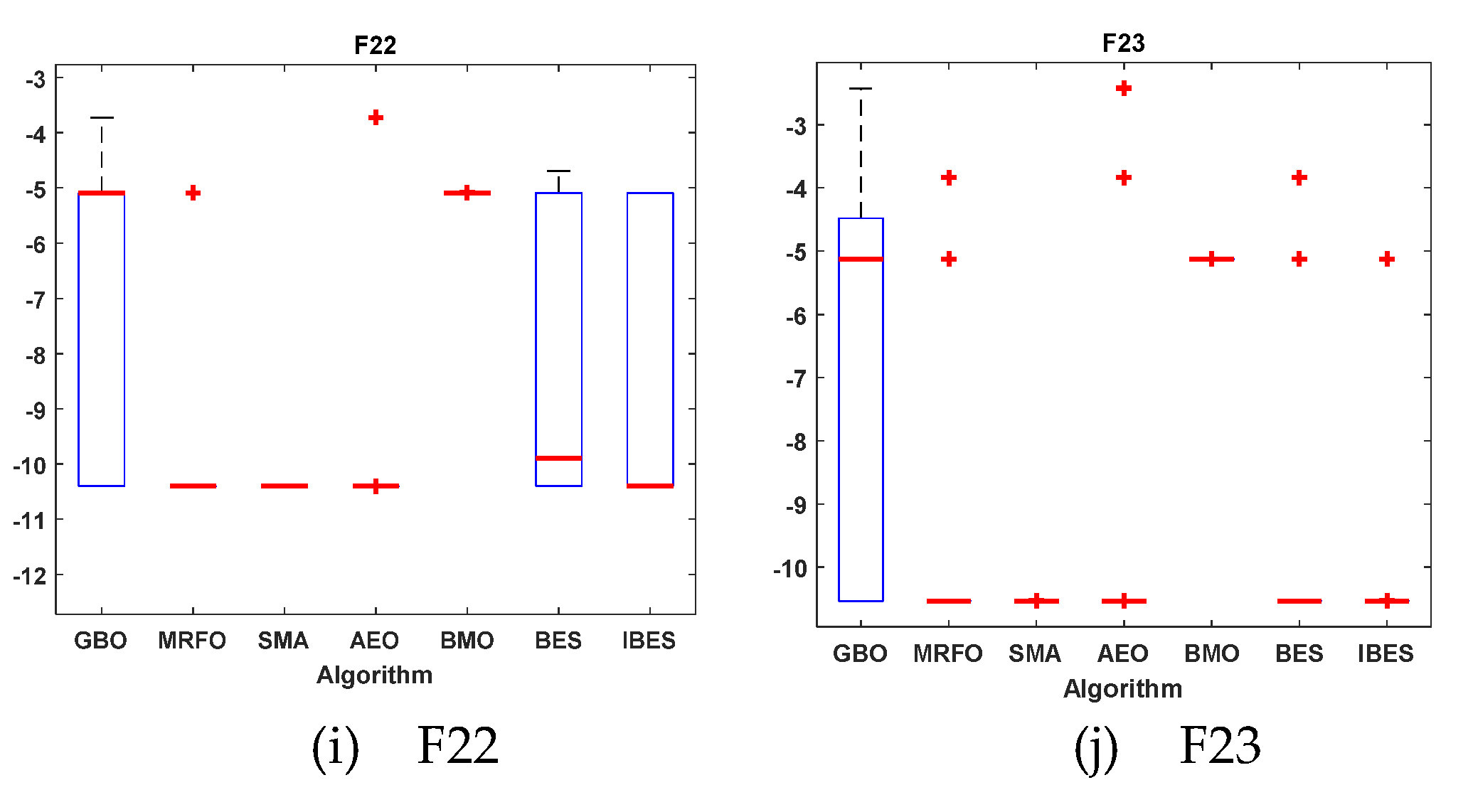
The IBES was tested and evaluated on different benchmark functions. The results for the IBES algorithm were compared with other recent optimization algorithms. Table 1 presents the parameters of all compared algorithms (IBES, BES, GBO, MRFO, SMA, and BMO). Table 2 presents the statistical results of all compared algorithms when applied for unimodal benchmark functions named from F1 to F7. The best values, shown in bold, were achieved with IBES and BES, but the IBES algorithm results were better than those of BES. The statistical results of multimodal benchmark functions, named from F8 to F13, are presented in Table 3. The statistical results of composite benchmark functions, named from F14 to F23, are presented in Table 4. Figure 9 presents the qualitative metrics for the F2, F4, F6, F8, F12, F15, and F18 functions, including 2D views of the functions, search histories, average fitness histories, and convergence curves. Figure 10, Figure 11 and Figure 12 present boxplots of the unimodal benchmark functions, multimodal benchmark functions, and composite benchmark functions, respectively. The IBES achieved the best values with the unimodal function with a percentage of 75% and for the composite function with a percentage of 60%; however, with multimodal functions, SMA won with a percentage of 70.8%. Table 5 presents the percentages for the best results compared to the total statistical results for unimodal, multimodal, and composite functions for all algorithms.

Table 1. Parameter settings of the selected techniques.

Algorithms	Parameters Setting
Common settings	Population size: nPop = 50
	Maximum iterations: Max_iter = 100
	Number of independent runs = 30
GBO	Probability Parameter: Pr = 0.5
MRFO	S = 2
SMA	Z = 0.03
BMO	Pl = 7
BES	C1, C2, α = 2, a = 10, R = 1.5
IBES	C1, C2 =2, a = 10, R = 1.5

Table 2. Results for unimodal benchmark functions.

Function		GBO	MRFO	SMA	AEO	BMO	BES	IBES
F1	Best	1.00 × 10−23	1.23 × 10−90	6.92 × 10−156	7.97 × 10−42	2.11 × 10−141	0	0
	Worst	9.21 × 10−21	1.64 × 10−80	8.85 × 10−85	2.26 × 10−33	6.12 × 10−123	0	0
	Mean	1.92 × 10−21	9.98 × 10−82	4.59 × 10−86	2.50 × 10−34	3.10 × 10−124	0	0
	std	2.79 × 10−21	3.68 × 10−81	1.98 × 10−85	5.82 × 10−34	1.37 × 10−123	0	0
F2	Best	4.32 × 10−13	1.12 × 10−45	4.30 × 10−79	1.36 × 10−22	6.59 × 10−73	0	0
	Worst	1.03 × 10−10	5.26 × 10−42	3.70 × 10−46	6.59 × 10−17	1.47 × 10−62	1.37 × 10−270	4.47 × 10−303
	Mean	1.96 × 10−11	5.11 × 10−43	1.85 × 10−47	9.84 × 10−18	7.69 × 10−64	6.85 × 10−272	2.73 × 10−304
	std	2.66 × 10−11	1.20 × 10−42	8.28 × 10−47	1.84 × 10−17	3.29 × 10−63	0	0
F3	Best	5.08 × 10−50	2.87 × 10−127	3.06 × 10−134	3.44 × 10−38	3.84 × 10−148	0	0
	Worst	7.79 × 10−45	2.24 × 10−117	7.31 × 10−63	2.20 × 10−30	1.60 × 10−123	0	0
	Mean	4.20 × 10−46	1.54 × 10−118	6.45 × 10−64	2.84 × 10−31	9.27 × 10−125	0	0
	std	1.74 × 10−45	5.05 × 10−118	2.00 × 10−63	6.19 × 10−31	3.55 × 10−124	0	0
F4	Best	3.69 × 10−11	8.16 × 10−46	6.02 × 10−69	2.55 × 10−21	6.93 × 10−70	0	0
	Worst	5.29 × 10−10	1.66 × 10−40	1.39 × 10−35	8.30 × 10−17	1.55 × 10−62	1.51 × 10−260	1.60 × 10−294
	Mean	2.49 × 10−10	1.72 × 10−41	7.81 × 10−37	1.38 × 10−17	1.19 × 10−63	7.56 × 10−262	8.32 × 10−296
	std	1.68 × 10−10	3.92 × 10−41	3.10 × 10−36	2.44 × 10−17	3.63 × 10−63	0	0
F5	Best	26.20355	25.89819	28.4411	26.41348	28.39232	23.42343	23.49114
	Worst	28.72399	27.07267	28.91551	27.87792	28.83662	25.76698	25.32653
	Mean	27.28987	26.39814	28.61466	27.1144	28.61644	24.26849	24.66361
	std	0.554629	0.344638	0.162272	0.409592	0.125605	0.6296	0.461041
F6	Best	0.03963	0.001831	0.008039	0.090625	2.424723	6.7 × 10−7	1.43 × 10−5
	Worst	0.228144	0.255766	1.4177	0.66915	3.710475	7.96 × 10−5	0.249381
	Mean	0.102408	0.02639	0.679072	0.333799	3.174803	1.79 × 10−5	0.03938
	std	0.049555	0.055015	0.458967	0.173604	0.395355	2.61 × 10−5	0.084456
F7	Best	0.000839	2.28 × 10−5	2.68 × 10−5	9.34 × 10−5	8.21 × 10−6	1.58 × 10−5	2.25 × 10−6
	Worst	0.009435	0.00129	0.001258	0.009584	0.00065	0.000348	0.00031
	Mean	0.002914	0.000388	0.000551	0.001969	0.000201	0.000142	8.49 × 10−5
	std	0.001943	0.0003	0.000371	0.002193	0.000168	9.99 × 10−5	7.8 × 10−5

Table 3. Results for multimodal benchmark functions.

Function		GBO	MRFO	SMA	AEO	BMO	BES	IBES
F8	Best	−1830.71	−1608.25	−1909.05	−1759.19	−1454.34	−1777.18	−1731.16
	Worst	−1642.02	−1250.53	−1905.97	−1400.39	−800.961	−1043.35	−1354.55
	Mean	−1720.61	−1460.49	−1908.16	−1608.48	−1161.96	−1503.62	−1543.11
	std	43.85651	95.02298	0.79786	93.70687	155.4007	256.3825	100.2304
F9	Best	0	0	0	0	0	0	0
	Worst	0	0	0	0	0	0	0
	Mean	0	0	0	0	0	0	0
	std	0	0	0	0	0	0	0
F10	Best	8.88 × 10−16	8.88 × 10−16	8.88 × 10−16	8.88 × 10−16	8.88 × 10−16	8.88 × 10−16	8.88 × 10−16
	Worst	3.7 × 10−8	8.88 × 10−16	8.88 × 10−16	4.44 × 10−15	8.88 × 10−16	20	20
	Mean	4.09 × 10−9	8.88 × 10−16	8.88 × 10−16	1.24 × 10−15	8.88 × 10−16	18	11
	std	8.72 × 10−9	0	0	1.09 × 10−15	0	6.15587	10.20836
F11	Best	0	0	0	0	0	0	0
	Worst	2.04 × 10−9	0	0	0	0	0	0
	Mean	1.02 × 10−10	0	0	0	0	0	0
	std	4.56 × 10−10	0	0	0	0	0	0
F12	Best	0.000366	6.18 × 10−5	1.52 × 10−5	0.001042	0.141918	2.91 × 10−9	6.53 × 10−6
	Worst	0.00209	0.000955	0.018428	0.004707	0.430386	3.41 × 10−7	9.95 × 10−5
	Mean	0.001236	0.000306	0.003839	0.00285	0.233487	1.04 × 10−7	4.13 × 10−5
	std	0.000492	0.000203	0.00548	0.001198	0.072019	1.21 × 10−7	2.55 × 10−5
F13	Best	0.104263	0.106128	0.001662	0.530081	2.975561	2.24745	1.95995
	Worst	0.475712	2.967327	2.530503	2.970408	2.984392	2.966102	2.968414
	Mean	0.2188	2.328378	0.789293	1.665532	2.980695	2.904654	2.916155
	std	0.089562	1.053699	0.891767	0.894496	0.002041	0.192063	0.225068

The best values obtained are in bold.

Table 4. Results for composite benchmark functions.

Function		GBO	MRFO	SMA	AEO	BMO	BES	IBES
F14	Best	0.998004	0.998004	0.998004	0.998004	0.998004	0.998004	0.998004
	Worst	3.96825	0.998004	1.992031	0.998004	12.67051	12.67051	0.998004
	Mean	1.196218	0.998004	1.047705	0.998004	9.589146	1.978449	0.998004
	std	0.68919	4.62 × 10−11	0.222271	1.53 × 10−16	4.153516	2.643447	1.91 × 10−16
F15	Best	0.000307	0.000308	0.000309	0.000307	0.000308	0.000307	0.000307
	Worst	0.020363	0.020364	0.001579	0.001223	0.00073	0.020363	0.001223
	Mean	0.001647	0.001347	0.00081	0.000359	0.000406	0.001356	0.000358
	std	0.004469	0.004476	0.000409	0.000204	0.000123	0.004479	0.000204
F16	Best	−1.03163	−1.03163	−1.03163	−1.03163	−1.03163	−1.03163	−1.03163
	Worst	−1.03163	−1.03163	−1.03163	−1.03163	−1.03163	−1.03163	−1.03163
	Mean	−1.03163	−1.03163	−1.03163	−1.03163	−1.03163	−1.03163	−1.03163
	std	8.82 × 10−17	1.69 × 10−16	3.00 × 10−8	1.14 × 10−16	2.31 × 10−9	2.16 × 10−16	2.10 × 10−16
F17	Best	0.397887	0.397887	0.397887	0.397887	0.397887	0.397887	0.397887
	Worst	0.397887	0.397887	0.39789	0.397887	0.397888	0.397887	0.397887
	Mean	0.397887	0.397887	0.397888	0.397887	0.397887	0.397887	0.397887
	std	0	0	8.28 × 10−7	0	4.58 × 10−8	0	0
F18	Best	3	3	3	3	3	3	3
	Worst	3	3	3	3	3.000023	3	3
	Mean	3	3	3	3	3.000002	3	3
	std	3.8 × 10−15	3.54 × 10−15	1.09 × 10−7	3.15 × 10−15	5.5 × 10−6	1.37 × 10−15	1.04 × 10−15
F19	Best	−0.30048	−0.30047	−0.30048	−0.30048	−0.30048	−0.30048	−0.30048
	Worst	−0.30048	−0.30033	−0.30048	−0.30047	−0.30048	−0.30048	−0.30048
	Mean	−0.30048	−0.30044	−0.30048	−0.30048	−0.30048	−0.30048	−0.30048
	std	1.14 × 10−16	3.3 × 10−5	1.14 × 10−16	1.71 × 10−6	1.14 × 10−16	1.14 × 10−16	1.14 × 10−16
F20	Best	−3.322	−3.322	−3.32198	−3.322	−3.32002	−3.322	−3.322
	Worst	−3.2031	−3.2031	−3.32156	−3.2031	−3.02059	−3.2031	−3.2031
	Mean	−3.28633	−3.26255	−3.32178	−3.26849	−3.27455	−3.29822	−3.28633
	std	0.055899	0.060991	0.000132	0.060685	0.082702	0.048793	0.055899
F21	Best	−10.1532	−10.1532	−10.153	−10.1532	−5.05519	−10.1532	−10.1532
	Worst	−5.0552	−5.0552	−10.1427	−2.63047	−5.05463	−5.0552	−5.05483
	Mean	−7.60386	−9.38449	−10.1506	−9.77706	−5.05506	−7.60275	−8.1162
	std	2.614875	1.865999	0.002857	1.682133	0.000137	2.613742	2.559513
F22	Best	−10.4029	−10.4029	−10.4028	−10.4029	−5.08765	−10.4029	−10.4029
	Worst	−3.7243	−5.08767	−10.3968	−3.7243	−5.0863	−4.68994	−5.08767
	Mean	−7.34321	−9.33989	−10.4008	−10.069	−5.08739	−7.94017	−8.01313
	std	2.867583	2.18134	0.001674	1.493389	0.000345	2.695609	2.710688
F23	Best	−10.5364	−10.5364	−10.536	−10.5364	−5.12847	−10.5364	−10.5364
	Worst	−2.42734	−3.83543	−10.5284	−2.42173	−5.12696	−3.83543	−5.12848
	Mean	−7.11694	−9.39017	−10.534	−9.39017	−5.12808	−9.38996	−9.99511
	std	3.259278	2.36602	0.001722	2.811921	0.000466	2.365915	1.664354

Figure 9. Qualitative metrics for the (a) F2, (b) F4, (c) F6, (d) F8, (e) F12, (f) F15, and (g) F18 functions: 2D views of the functions, search histories, average fitness histories, and convergence curves.

Figure 10. Boxplots for all algorithms for unimodal benchmark functions (a) F1, (b) F2, (c) F3, (d) F4, (e) F5, (f) F6, and (g) F7.

Figure 11. Boxplots for all algorithms for multimodal benchmark functions (a) F8, (b) F10, (c) F12, and (d) F13.

Figure 12. Boxplots for all algorithms for composite benchmark functions (a) F14, (b) F15, (c) F16, (d) F17, (e) F18, (f) F19, (g) F20, (h) F21, (i) F22, and (j) F23.

Table 5. The percentages of the best results compared to the total statistical results for unimodal, multimodal, and composite functions for all algorithms.

	IBES	BES	SMA	MBO	AEO	MRFO	GBO
Unimodal	75%	64.2%	0%	3.5%	0%	0%	0%
Multimodal	37.5%	54.1%	70.8%	54.1%	37.5%	50%	33.3
Composite	60%	50%	52.5%	40%	52.5%	42.5%	52.5

The bold indicates to the highest percentage.

4. Simulation Results

The analysis of the simulation results was performed to focus on different issues: the first issue was, on the one hand, the comparison between the improved algorithm and the original one (BES) and, on the other hand, the comparison between the modified triple diode model (MTDM) and the original triple diode model (TDM). This issue was covered in task 1. In this task, the results of the IBES and BES were compared with regard to the estimation of the parameters of the MTDM and TDM for real data from an RTC furnace solar cell [7]. The second issue was the comparison of the performance of the IBES and other recent algorithms.

4.1. Task 1: Comparison between IBES and BES for the MTDM and TDM

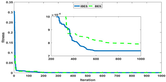
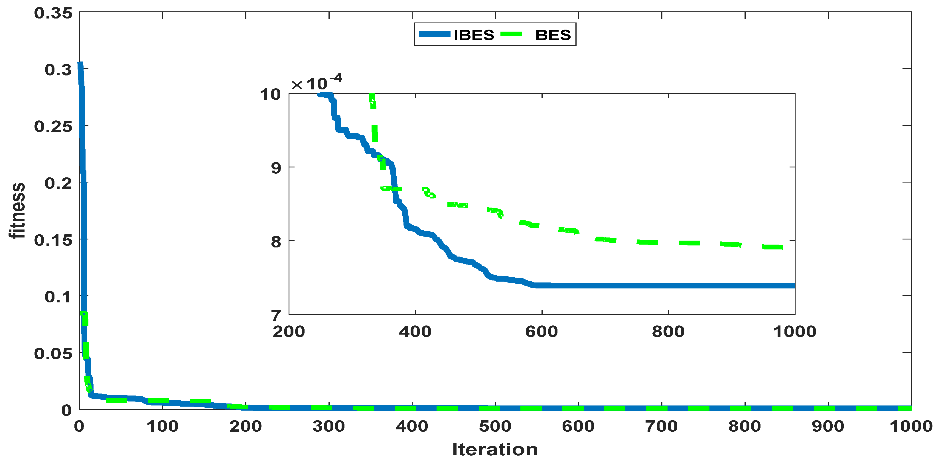
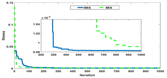
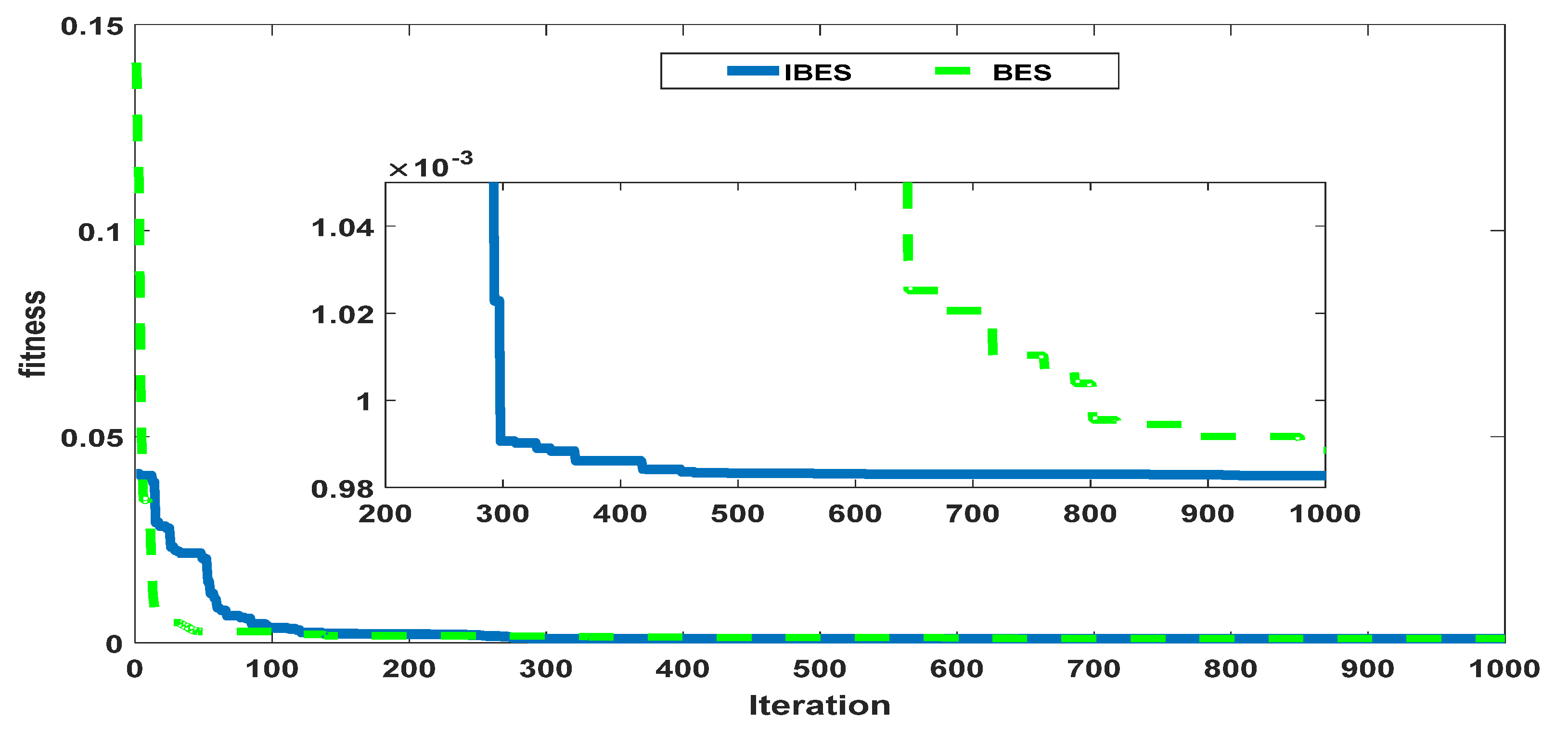
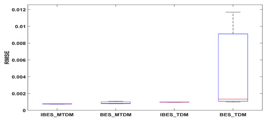
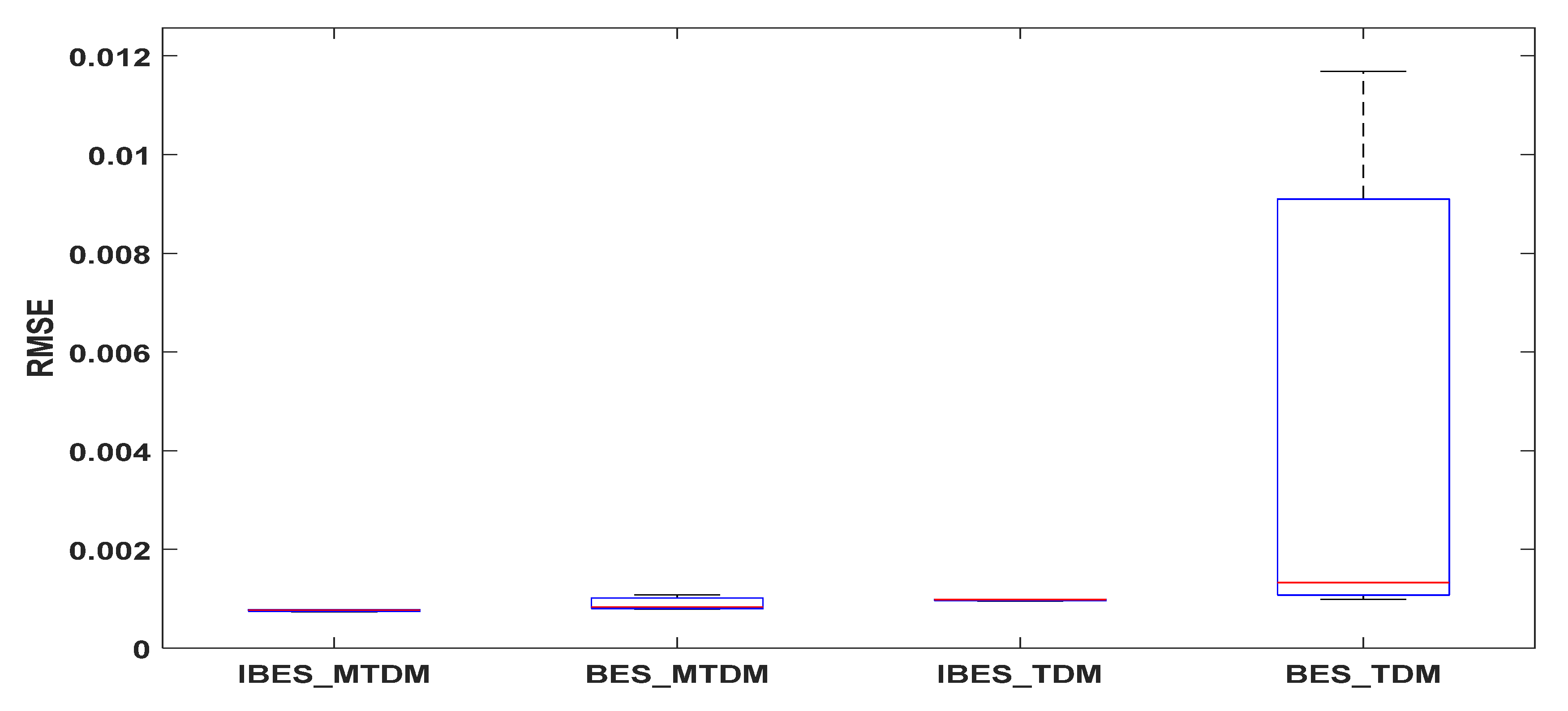
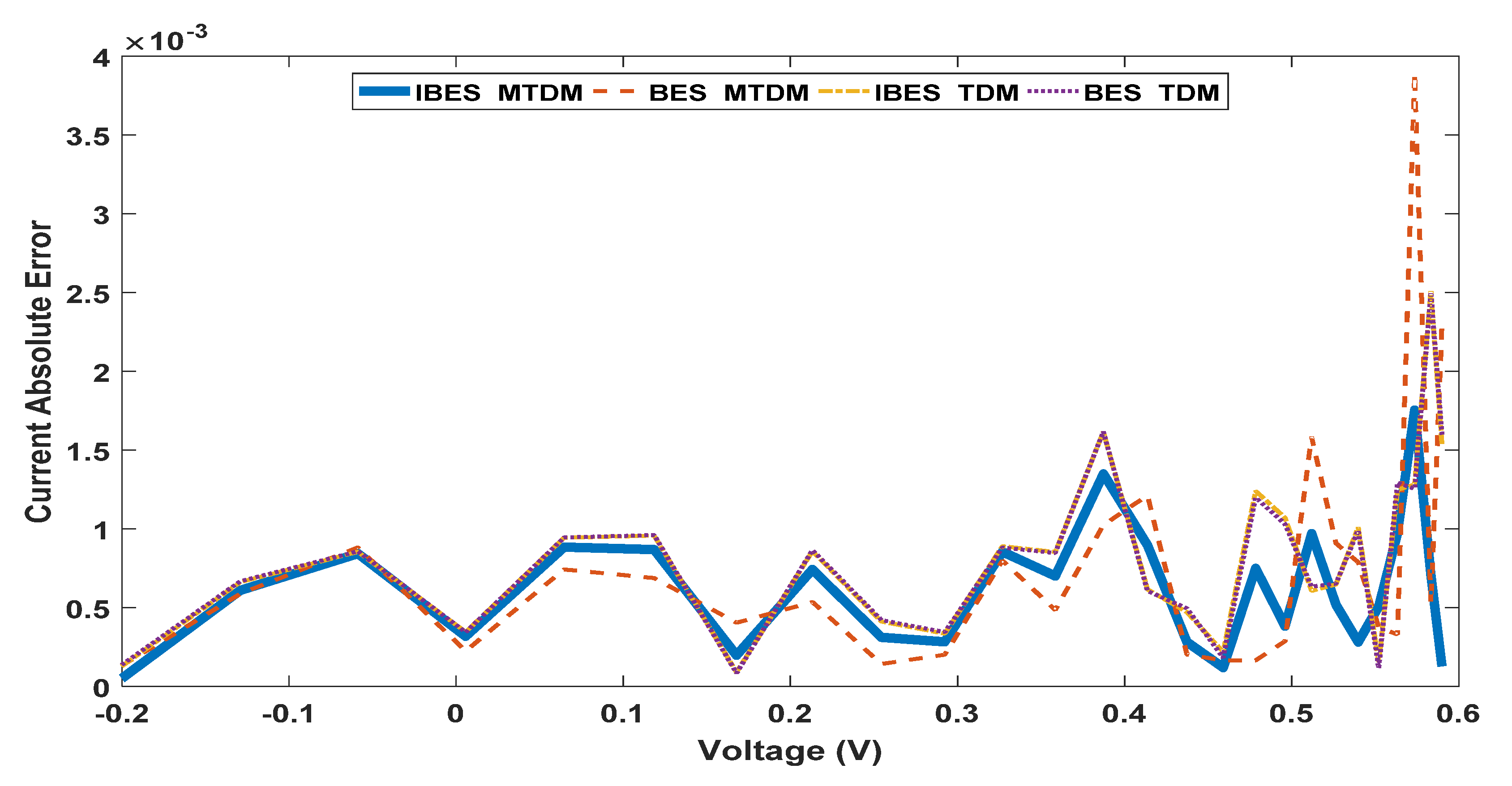
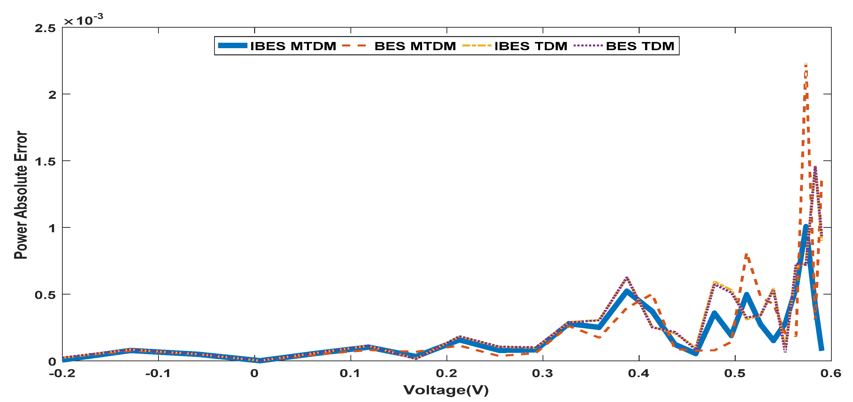
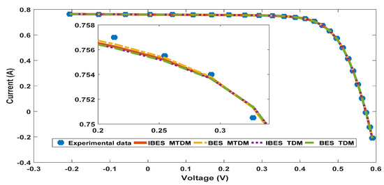
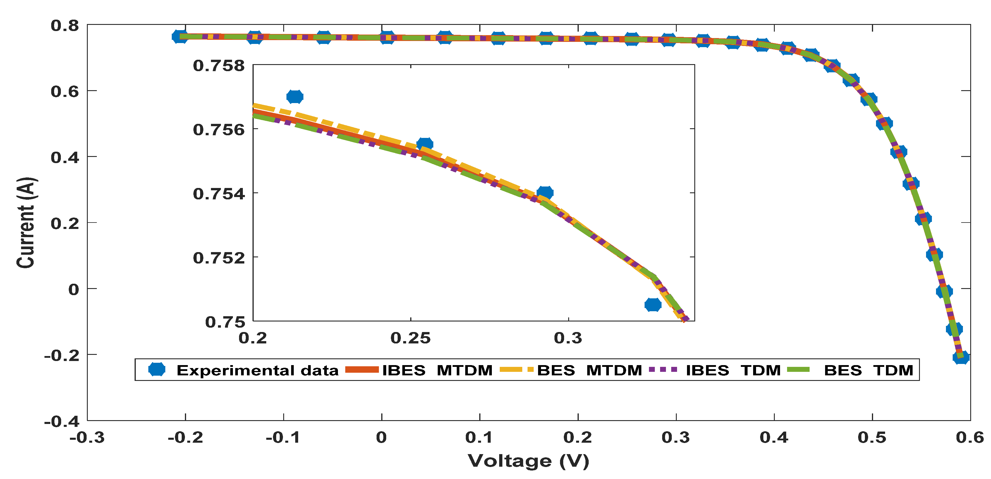
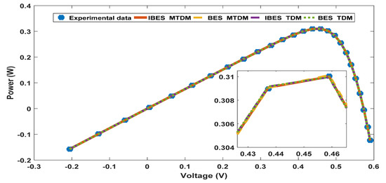
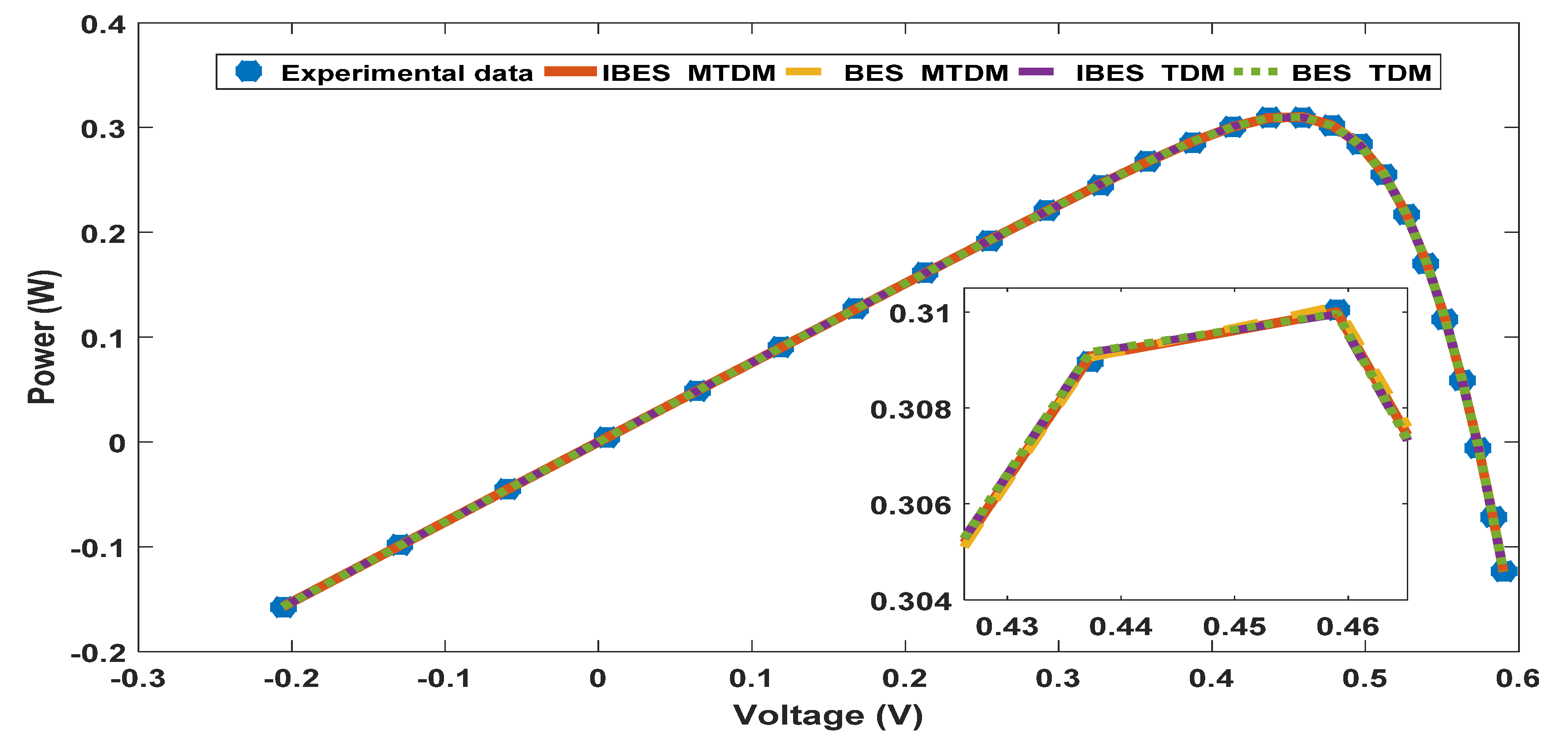
In this task the IBES and BES were applied to estimate the parameters of the MTDM and TDM. The objective functions for the TDM and MTDM are described in Equations (13) and (15), respectively. The measured data from a 57 mm diameter commercial silicon R.T.C. France solar cell (under 1000 W/m² at 33 °C) [7] were used. In Table 6 the estimations for the 10 parameters of the MTDM by IBES and BES are presented. The estimations for the nine parameters of the TDM by IBES and BES are also presented in Table 6. From the RMSE (Equation (20)), it can be seen that the results of the IBES were more accurate than those of the BES in the two cases. The convergence curves of IBES and BES for the MTDM TDM are shown in Figure 13 and Figure 14, respectively. The statistical results of the RMSE values calculated for 30 independent runs are presented in Table 7. The statistical results are presented in boxplots for each algorithm in Figure 15. The values for the current absolute error (IAE) and the power absolute error (PAE) (Equation (21)) for all cases are presented in Figure 16 and Figure 17, respectively. From these results, it can be concluded that the results of both the IBES and BES for MTDM were more accurate than for TDM; moreover, the IBES results were more accurate than those of BES for the MTDM and TDM. By comparing the obtained results achieved for the IBES for MTDM with the results from [5], which used EHO to estimate the parameters for the MTDM, we can see that the IBES results are better than those of the EHO, as the RMSE obtained by EHO was 0.001233. Reference [5] was selected for this comparison as it used the same optimization condition. According to our review of the literature, the RMSE value obtained by the IBES for the MTDM (0.000739055) is better than a lot of recent optimization algorithms. For further comparison, current vs. voltage and power vs. voltage characteristics curves for real system MTDMs and TDMs estimated by the IBES and BES are presented in Figure 18 and Figure 19, respectively.

$$RMSE=\sqrt{\frac{1}{N}{\displaystyle \sum _{K=1}^N{f}^2(V,I,X)}}$$

(20)

$$IAE=\sqrt[2]{{(I_{err})}^2}, PAE=\sqrt[2]{{(P_{err})}^2}$$

(21)

Table 6. Results of the IBES and BES for the MTDM and TDM for a furnace.

Algorithm	IBES MTDM	BES MTDM	IBES TDM	BES TDM
Rs (Ω)	0.013865736	0.03027	0.036664	0.036291
Rsh (Ω)	55.47156858	58.23366	55.00941	54.40551
Iph (A)	0.760473235	0.760768	0.76079	0.760777
Isd1 (A)	1.00 × 10−10	4.12 × 10−10	9.73 × 10−8	3.32 × 10−7
Isd2 (A)	7.52 × 10−7	1.00 × 10−10	1.90 × 10−7	1.03 × 10−10
Isd3 (A)	1.00 × 10−10	1.12 × 10−6	6.30 × 10−7	1.13 × 10−10
N1	1.133059042	1.100636	1.27987	1.479641
N2	1.537322148	1.013835	1.187585	1.491094
N3	1.004574508	1.650876	1.729511	1.497359
Rsm	0.027870684	0.189638	------	------
RMSE	0.000739055	0.00079074727	0.0009826679	0.00098849305

Figure 13. The convergence curves for the IBES and BES for the MTDM.

Figure 14. The convergence curves of the IBES and BES for the TDM.

Table 7. Statistical results for the IBES applied to the MTDM and TDM and for the BES applied to the MTDM and TDM.

	Minimum	Average	Maximum	STD
IBES	0.000739	0.000764	0.000781	2.21 × 10−5
MTDM
BES	0.000791	0.000901	0.001078	0.000155
MTDM
IBES	0.000953	0.000973	0.000984	1.78 × 10−5
TDM
BES	0.000988	0.004668	0.011687	0.006081
TDM

Figure 15. Boxplot for the IBES applied to the MTDM and TDM and the BES applied to the MTDM and TDM for 30 independent runs.

Figure 16. IAE for the IBES and BES for all cases.

Figure 17. PAE for the IBES and BES for all cases.

Figure 18. Current–voltage curve for the experimental data and for the MTDM, and TDM currents estimated by the IBES and BES.

Figure 19. Power–voltage curve for the experimental data and for the MTDM and TDM currents estimated by the IBES and BES.

4.2. Task 2: Comparison between the IBES and Recent Algorithms

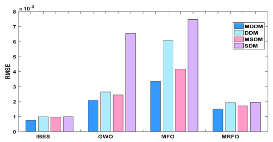
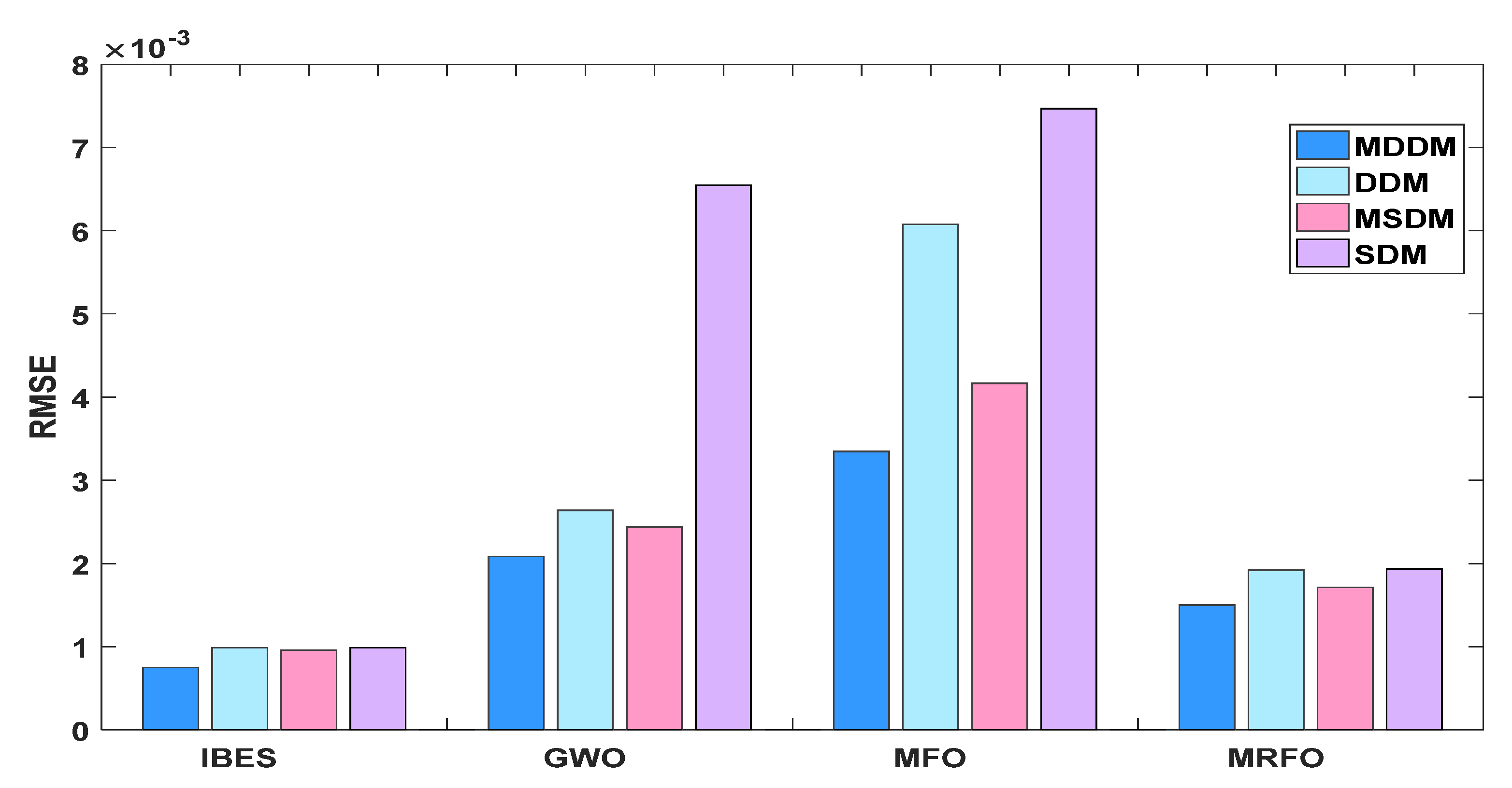
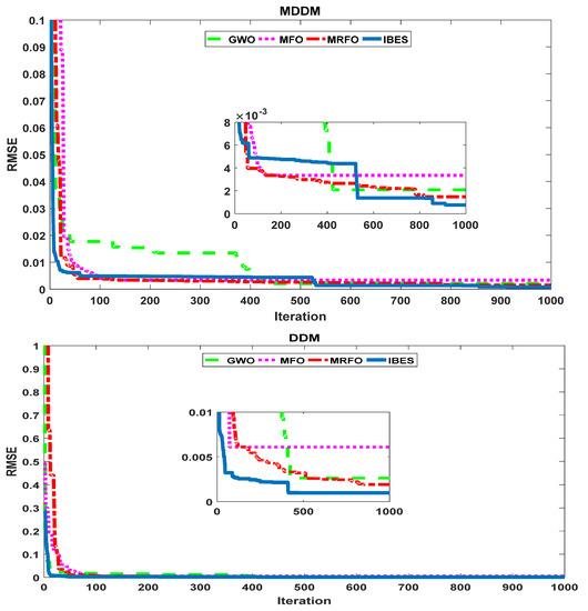
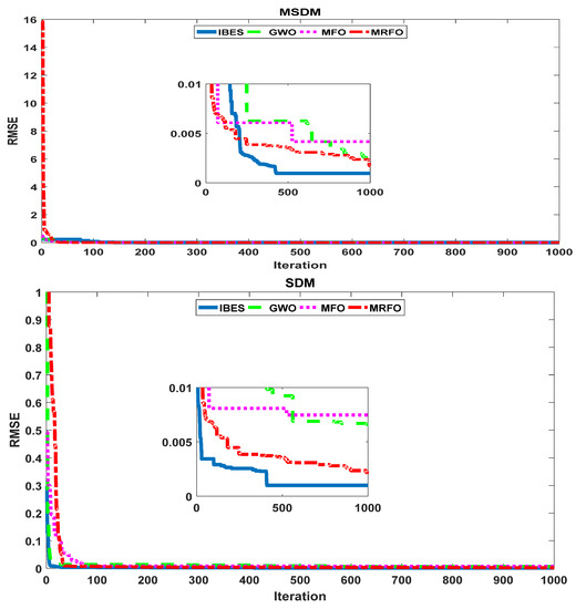
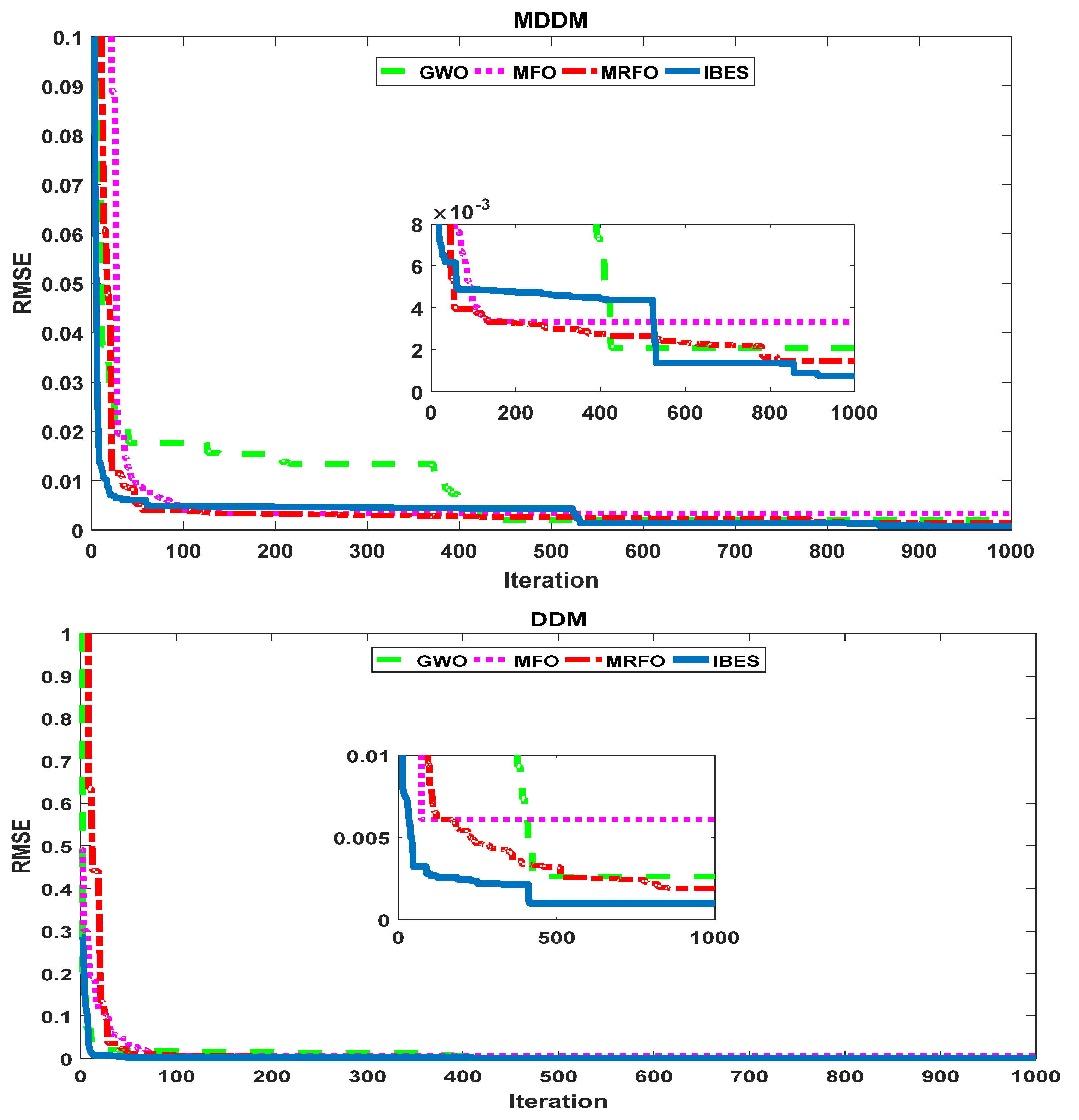
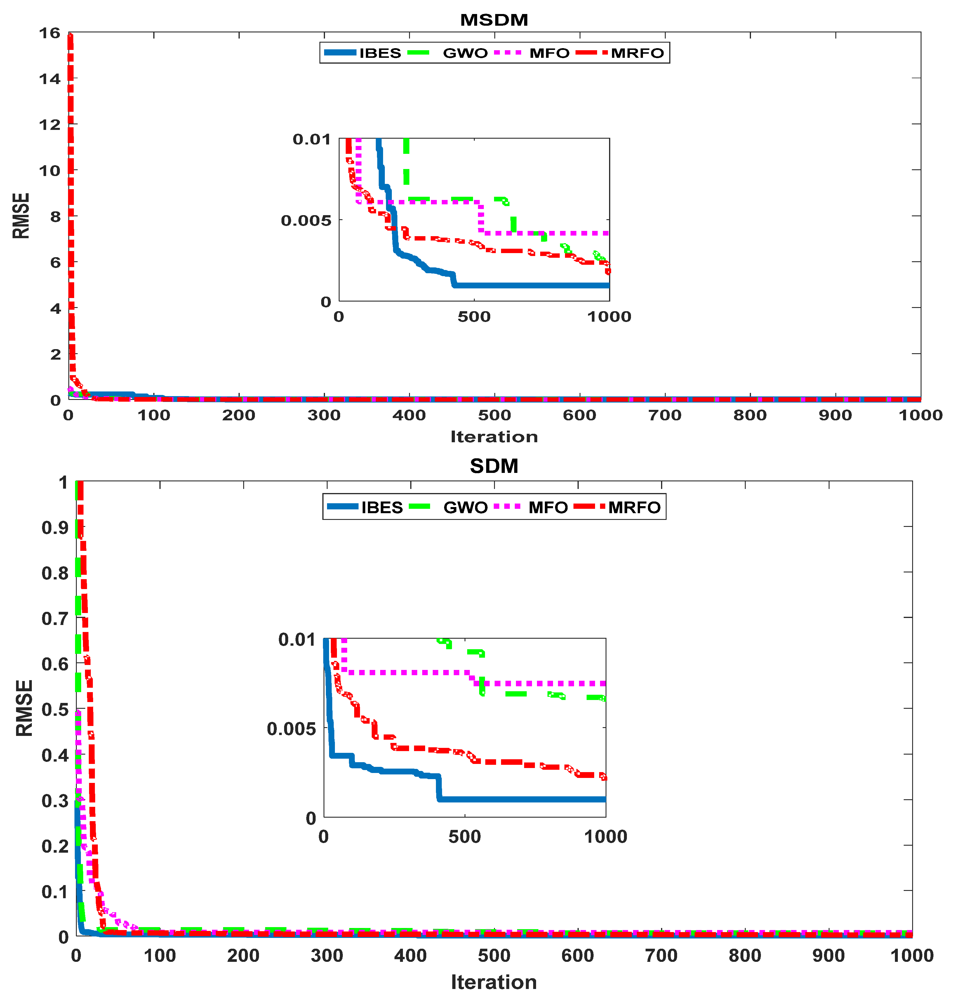
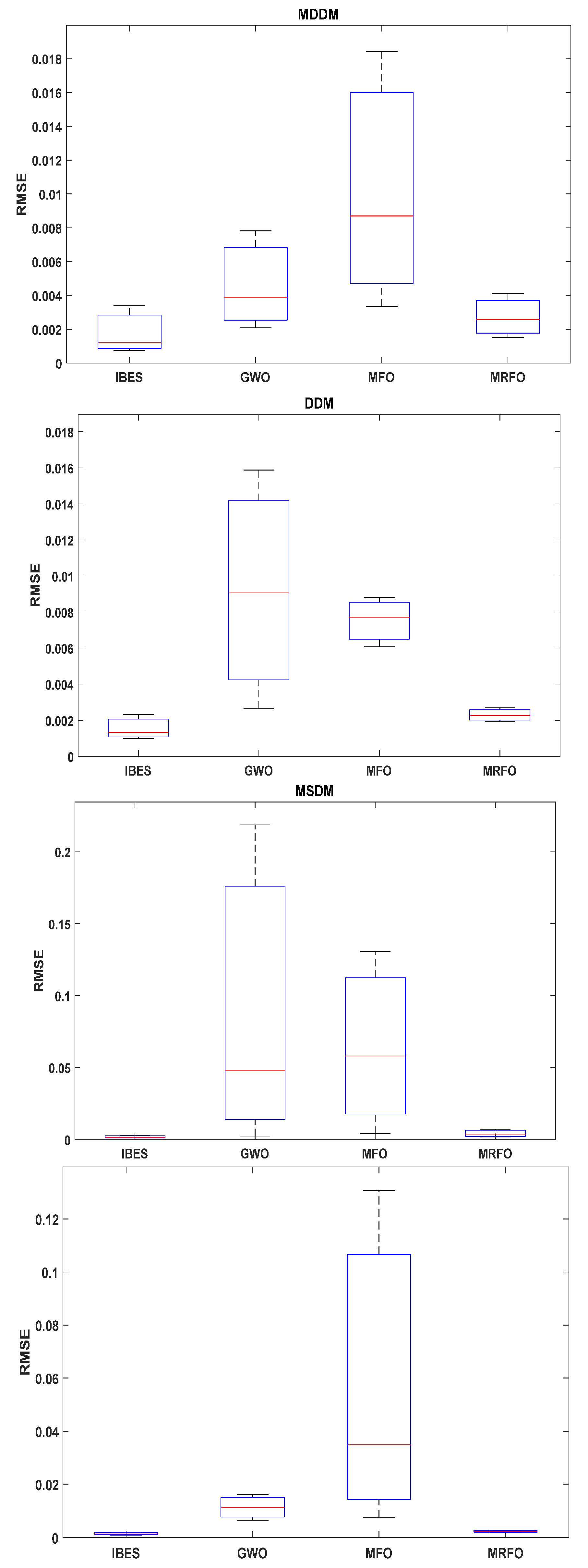
In this task, we compared the performance of the IBES and recent algorithms with regard to the estimation of the parameters of the MDDM, MSDM, DDM, and SDM for an RTC furnace solar cell. In Table 8 the parameters estimated for the MDDM, DDM, MSDM, and SDM by IBES and other algorithms are presented. The RMSEs for all compared algorithms and models are also presented in Table 8. The best RMSE values are highlighted in bold. From Table 8, it can be seen that the MDDM had more accurate parameters than the DDM, MSDM, or SDM. The lowest RMSE was recorded for the IBES. Figure 20 summarizes the results in Table 8 in graphical form. By comparing the results obtained for the IBES for the MDDM with the results from [5], which used EHO to estimate the parameters for the MDDM, it can be seen that the IBES results were better than those of EHO, as the RMSE obtained by the EHO was 0.001557. The convergence curves for all compared algorithms and models are shown in Figure 21. The statistical results of the RMSE values calculated for 30 independent runs are presented in Table 9. The statistical results are presented in boxplots for each algorithm in Figure 22.

Table 8. Estimated parameters and RMSE values of the IBES, GWO, MFO, and MRFO applied to the MDDM, DDM, MSDM, and SDM.

		Parameters and RMSE
Algorithm	Model	Rs (Ω)	Rsh (Ω)	Iph (A)	Isd1 (A)	Isd2 (A)	N1	N2	Rsm	RMSE
IBES	MDDM	0.015196	54.05261	0.760494	1.00 × 10−10	6.69 × 10−7	1.00	1.525277	0.02792	0.000749
	DDM	0.036372	53.72365	0.760779	3.23 × 10−7	1.00 × 10−10	1.4770	1.428625	------	0.000986
	MSDM	0.032091	54.30519	0.760713	3.71 × 10−7	------	1.4835	------	0.00352	0.000961
	SDM	0.036377	53.71853	0.760776	3.23 × 10−7	------	1.4768	------	------	0.000986
GWO	MDDM	0.043886	511.3305	0.759336	1.89 × 10−10	5.31 × 10−6	1.0021	1.956081	0.017201	0.002084
	DDM	0.041921	999.9198	0.760812	7.43 × 10−6	1.54 × 10−10	2	1	------	0.002637
	MSDM	0.023214	483.3966	0.757734	6.85 × 10−7	------	1.5352	------	0.008153	0.002442
	SDM	0.020609	319.2442	0.762942	6.16 × 10−6	------	1.8478	------	------	0.006547
MFO	MDDM	0.007956	1000	0.761301	1.37 × 10−5	1.00 × 10−10	2	1	0.128316	0.003346
	DDM	0.034107	1000	0.763016	1.00 × 10−5	1.00 × 10−10	2	1	------	0.006079
	MSDM	0.001	1000	0.761623	8.24 × 10−6	------	1.8539	------	0.012323	0.004165
	SDM	0.018046	1000	0.76332	9.06 × 10−6	------	1.9107	------	------	0.007466
MRFO	MDDM	0.034095	444.1404	0.76047	6.67 × 10−7	5.69 × 10−6	1.5526	1.725619	1.985829	0.001499
	DDM	0.03375	132.5792	0.759954	6.45 × 10−7	1.62 × 10−7	1.5509	1.954467	------	0.001918
	MSDM	0.013187	88.00777	0.760272	1.57 × 10−6	------	1.6247	------	0.010754	0.001712
	SDM	0.03388	103.6053	0.760412	6.38 × 10−7	------	1.5479	------	------	0.001937

Figure 20. Comparison between the RMSE values of the IBES, GWO, MFO, and MRFO applied to the MDDM, DDM, MSDM, and SDM.

Figure 21. The convergence curves of the IBES, GWO, MFO, and MRFO applied to the MDDM, DDM, MSDM, and SDM.

Table 9. Statistical results for the IBES, GWO, MFO, and MRFO applied to the MDDM, DDM, MSDM, and SDM.

Algorithm	Model	Minimum	Average	Maximum	STD
IBES	MDD	0.000749	0.001201	0.003378	0.000895
	DD	0.000986	0.001324	0.002309	0.000548
	MSD	0.000961	0.001507	0.002847	0.000761
	SD	0.000986	0.001392	0.00193	0.000405
GWO	MDD	0.002084	0.003891	0.007816	0.002258
	DD	0.002637	0.009064	0.01587	0.00623
	MSD	0.002442	0.04817	0.218713	0.095358
	SD	0.006547	0.011483	0.016251	0.004853
MFO	MDD	0.003346	0.008697	0.018428	0.00574
	DD	0.006079	0.00772	0.008818	0.001498
	MSD	0.004165	0.058033	0.130639	0.066501
	SD	0.007466	0.034848	0.130639	0.053726
MRFO	MDD	0.001499	0.002572	0.00409	0.000967
	DD	0.001918	0.002255	0.002697	0.000281
	MSD	0.001712	0.003704	0.007213	0.002271
	SD	0.001937	0.002386	0.002848	0.000404

Figure 22. Boxplots of the IBES, GWO, MFO, and MRFO applied to the MDDM, DDM, MSDM and SDM.

5. Conclusions

In this paper, an improvement for the BES algorithm was proposed. The improved algorithm is called the IBES algorithm. The improvement is based on creating varied values for the learning parameter in each iteration. This improvement enhances the exploration and exploitation in the IBES technique. The proposed algorithm was evaluated through 23 different benchmark functions and applied for parameter estimation of different PV models. The IBES was tested with challenging optimization problems from the literature and through parameter estimation of the MTDM and TDM, which considered the most complex PV models and compared the IBES with the original BES algorithm; this was in the first task. In task 2, the IBES was applied to estimate the parameters for the MDDM, DDM, MSDM, and SDM and the results were compared with recent optimization algorithms. The real data measured from a 57 mm diameter commercial silicon R.T.C. France solar cell were used for all tasks. The comparisons in all tasks involved comparing different evaluation parameters; for example, RMSE and IAE and PAE and statistical analysis. For a more comprehensive comparison, the IBES results in tasks 1 and 2 were compared with available recent studies that used the same examples and optimization conditions. The proposed algorithm achieved significant accuracy in comparison with the original algorithm and other recent algorithms. The achievements of the IBES will encourage the authors to apply the IBES to estimate the parameters of highly complicated PV cells, such as concentrated PV cells or large PV systems, in future work.

References

- Kumar, V.R.; Singh, S.K. Solar photovoltaic modelling and simulation: As a renewable energy solution. Energy Rep. 2018, 4, 701–712. [Google Scholar]
- Lyden, S.; Haque, M.E.; Gargoom, A.; Negnevitsky, M.; Muoka, P.I. Modelling and parameter estimation of photovoltaic cell. In Proceedings of the 22nd Australasian Universities Power Engineering Conference (AUPEC), Bali, Indonesia, 26–29 September 2012. [Google Scholar]
- Allam, D.; Yousri, D.A.; Eteiba, M.B. Parameters Extraction of the Three Diode Model for the Multi-crystalline Solar Cell/ Module Using Moth-Flame Optimization Algorithm. Energy Convers. Manag. 2016, 123, 535–548. [Google Scholar] [CrossRef] [Scilit]
- Chin, V.J.; Salam, Z.; Ishaque, K. Cell modelling and model parameters estimation techniques for photovoltaic simulator application: A review. Appl. Energy 2015, 154, 500–519. [Google Scholar] [CrossRef] [Scilit]
- Bayoumi, A.S.; El-Sehiemy, R.A.; Mahmoud, K.; Lehtonen, M.; Darwish, M.M.F. Assessment of an Improved Three-Diode against Modified Two-Diode Patterns of MCS Solar Cells Associated with Soft Parameter Estimation Paradigms. Appl. Sci. 2021, 11, 1055. [Google Scholar] [CrossRef] [Scilit]
- Abdelminaam, D.S.; Said, M.; Houssein, E.H. Turbulent Flow of Water-Based Optimization Using New Objective Function for Parameter Extraction of Six Photovoltaic Models. IEEE Access 2021, 9, 35382–35398. [Google Scholar] [CrossRef] [Scilit]
- Ramadan, A.; Kamel, S.; Korashy, A.; Yu, J. Photovoltaic Cells Parameter Estimation Using an Enhanced Teaching–Learning-Based Optimization Algorithm. Iran. J. Sci. Technol. Trans. Electr. Eng. 2019, 44, 767–779. [Google Scholar] [CrossRef] [Scilit]
- Abdelghany, R.Y.; Kamel, S.; Ramadan, A.; Sultan, H.; Rahmann, C. Solar Cell Parameter Estimation Using School-Based Optimization Algorithm. In Proceedings of the IEEE International Conference on Automation/XXIV Congress of the Chilean Association of Automatic Control (ICA-ACCA), Santiago, Chile, 22–26 March 2021. [Google Scholar]
- Ramadan, A.; Kamel, S.; Hussein, M.M.; Hassan, M.H. A New Application of Chaos Game Optimization Algorithm for Parameters Extraction of Three Diode Photovoltaic model. IEEE Access 2021, 9, 51582–51594. [Google Scholar] [CrossRef] [Scilit]
- Ahmed, A.Z.D.; Sultan, H.M.; Do, T.D.; Kamel, O.M.; Mossa, M.A. Coyote Optimization Algorithm for Parameters Estimation of Various Models of Solar Cells and PV Modules. IEEE Access 2020, 8, 111102–111140. [Google Scholar]
- Sharma, A.; Sharma, A.; Averbukh, M.; Jately, V.; Azzopardi, B. An Effective Method for Parameter Estimation of a Solar Cell. Electronics 2021, 10, 312. [Google Scholar] [CrossRef] [Scilit]
- Rezk, H.; Babu, T.S.; Al-Dhaifallah, M.; Ziedan, H.A. A robust parameter estimation approach based on stochastic fractal search optimization algorithm applied to solar PV parameters. Energy Rep. 2021, 7, 620–640. [Google Scholar] [CrossRef] [Scilit]
- Humada, A.M.; Darweesh, S.Y.; Mohammed, K.G.; Kamil, M.; Mohammed, S.F.; Kasim, N.K.; Tahseen, T.A.; Awad, O.I.; Mekhilef, S. Modeling of PV system and parameter extraction based on experimental data: Review and investigation. Solar Energy 2020, 199, 742–760. [Google Scholar] [CrossRef] [Scilit]
- Lv, X.; Wang, Y.; Deng, J.; Zhang, G.; Zhang, L. Improved Particle Swarm Optimization Algorithm Based on Last-Eliminated Principle and Enhanced Information Sharing. Comput. Intell. Neurosci. 2018, 2018, 5025672. [Google Scholar] [CrossRef] [Scilit] [PubMed]
- Wang, G.; Yuan, Y.; Guo, W. An Improved Rider Optimization Algorithm for Solving Engineering Optimization Problems. IEEE Access 2019, 7, 80570–80576. [Google Scholar] [CrossRef] [Scilit]
- Yassine, H.M.; Zahira, C. An Improved optimization Algorithm to Find Multiple Shortest Paths over Large Graph. In Proceedings of the Second International Conference on Embedded & Distributed Systems (EDiS), Oran, Algeria, 3 November 2020. [Google Scholar]
- Wang, J.S.; Li, S.X. An Improved Grey Wolf Optimizer Based on Differential Evolution and Elimination Mechanism. Sci. Rep. 2019, 9, 7181. [Google Scholar] [CrossRef] [Scilit] [PubMed]
- Alsattar, H.A.; Zaidan, A.A.; Zaidan, B.B. Novelmeta-heuristic bald eagle search optimisation algorithm. Artif. Intell. Rev. 2020, 53, 2237–2264. [Google Scholar] [CrossRef] [Scilit]
- Han, L.; Xu, C.; Huang, T.; Dang, X. Improved particle swarm optimization algorithm for high performance SPR sensor design”. Appl. Opt. 2021, 60, 1753–1760. [Google Scholar]
- Morris, T. Improved optimization algorithm for use in variational quantum eigensolvers. In Proceedings of the APS March Meeting, Boston, MA, USA, 4–8 March 2019. abstract id.E42.009. [Google Scholar]
- Bangyal, W.H.; Rauf, H.T.; Batool, H.; Bangyal, S.A.; Ahmed, J.; Pervaiz, S. An Improved Particle Swarm Optimization Algorithm with Chi-Square Mutation Strategy. Int. J. Adv. Comput. Sci. Appl. 2019, 10, 481–491. [Google Scholar] [CrossRef] [Scilit]
- Rajamohana, S.P.; Umamaheswari, K. Hybrid Optimization Algorithm of Improved Binary Particle Swarm Optimization (iBPSO) And Cuckoo Search for Review Spam Detection. In Proceedings of the 9th International Conference on Machine Learning and Computing, Singapore, 24–26 February 2017; pp. 238–242. [Google Scholar]
- Guo, W.; Liu, T.; Dai, F.; Xu, P. An Improved Whale Optimization Algorithm for Feature Selection. Appl. Intell. 2020, 62, 337–354. [Google Scholar] [CrossRef] [Scilit]
Publisher’s Note: MDPI stays neutral with regard to jurisdictional claims in published maps and institutional affiliations. |
© 2021 by the authors. Licensee MDPI, Basel, Switzerland. This article is an open access article distributed under the terms and conditions of the Creative Commons Attribution (CC BY) license (https://creativecommons.org/licenses/by/4.0/).