Numerical Investigation of a High-Pressure Submerged Jet Using a Cavitation Model Considering Effects of Shear Stress


1
Research Center of Fluid Machinery Engineering and Technology, Jiangsu University, Zhenjiang 212013, China
2
Institute of Fluid Engineering Equipment Technology, Jiangsu University, Zhenjiang 212009, China
3
College of Mechanical Engineering, Nantong University, Nantong 226019, China
*
Authors to whom correspondence should be addressed.
Processes 2019, 7(8), 541; https://doi.org/10.3390/pr7080541
Submission received: 29 June 2019
/
Revised: 7 August 2019
/
Accepted: 13 August 2019
/
Published: 15 August 2019
(This article belongs to the Section Advanced Digital and Other Processes)
Abstract
:In the current research, a high-pressure submerged cavitation jet is investigated numerically. A cavitation model is created considering the effect of shear stress on cavitation formation. As such, this model is developed to predict the cavitation jet, and then the numerical results are validated by high-speed photography experiment. The turbulence viscosity of the renormalization group (RNG) k-ε turbulence model is used to provide a flow field for the cavitation model. Furthermore, this model is modified using a filter-based density correction model (FBDCM). The characteristics of the convergent-divergent cavitation nozzle are investigated in detail using the current CFD simulation method. It is found that shear stress plays an important role in the cavitation formation in the high-pressure submerged jet. In the result predicted by the Zwart-Gerber-Belamri (ZGB) cavitation model, where critical static pressure is used for the threshold of cavitation inception, the cavitation bubble only appears at the nozzle outlet and the length of the cavity is much shorter than the actual length captured by the high-speed photography experiment. When the shear stress term is added to the critical pressure, the length of the predicted cavity is close to the experimental result and three phenomena of the jet are captured, namely, growth, shedding, and collapsing, which agrees well with the experimental high-speed image. According to the orthogonal analysis based on the simulation result, when the jet power is unchanged, the main geometry parameter of the divergent-convergent nozzle that affects the jet performance is the divergent angle. For the nozzle with three different divergent angles of 40°, 60°, and 80°, the one with the medium angle generates the most intensive cavitation cloud, while the small one shows the weakest cavitation performance. The obtained simulation result is confirmed by cavitation erosion tests of the Al1060 plate using these three nozzles.
1. Introduction
Cavitation is a well-known phenomenon in the field of fluid machinery. It can damage the hydraulic parts of the machines accompanied by noise and vibration [1,2,3]. Efforts have been made by researchers to avoid or reduce cavitation impact on pumps and turbines [4,5,6]. When the cavitation phenomenon is controlled and used properly, it will have enormous advantages in the engineering fields [7,8,9,10,11,12]. One of the commonly used techniques to generate intensive cavitation is a high-pressure submerged jet.
Research about the characteristics of high-pressure submerged cavitation jets has been mainly conducted by experimental methods. The effect of nozzle geometry, as well as jet parameters such as pressure and stand-off distance to the target, is investigated, aiming to improve the cavitation impact and promote the efficiency of the cleaning and cutting devices [13,14,15]. For the usage of cavitation peening, the residual stress, surface roughness and the micro-hardness of the peened metals are used to evaluate the performance of the jet. Since the jet velocity usually reaches more than 200 m/s, it is difficult to be detected by sensors. In addition, the flow region of the jet is filled with cavitation bubbles, which makes the Particle Image Velocimetry (PIV) difficult in process, where the bubbles may refract the laser light. Consequently, few experiments to detect the velocity field of high-pressure cavitation jets have been reported.
With the development of the CFD technique, the numerical simulation is becoming a common way to reveal the flow characteristic, which has advantages over experiments for investigating the theoretic phenomena in fluid dynamics. CFD codes have been widely used for predicting the performance of hydraulic machines [16,17]. Cavitating flow around hydrofoil or pumps is also simulated using multiphase flow models coupled with cavitation models based on the Rayleigh-Plesset equation. Qiang Guo et al. investigated the tip leakage vortex cavitation of a hydrofoil by coupling a cavitation model with a modified RANS model. It is found that the turbulence structure and the strength of the vortex have a great impact on the cavitating flow [18]. F. Khatami et al. [19] found that the compressibility of the gas-liquid mixture should be considered during the simulation of transient cavitating flow, and a set of URANS equations are used for the prediction of vortex cavitation in an elliptic hydrofoil. When the transient characteristics like vortex and shedding phenomenon are concerned, the turbulence model affects the simulation result to a large degree. The main reason is the compressibility and the large density gradient in the region that is close to cavitation clouds, and an accurate prediction on eddy viscosity is important for the simulation. Large Eddy Simulation (LES) has the ability to provide good results for cavitating simulation [20,21]. However, it is time-consuming and has a seriously high requirement for mesh quality. Consequently, different ways are developed to solve the transient cavitating flow using RANS models mainly by adjusting eddy viscosity which is usually over-predicted by RANS models [22,23,24].
The commonly used cavitation models that are available in most of the commercial algorithms are the Singhal model [25], Sauer model [26], and Zwart-Gerber-Belamri (ZGB) model [27]. The Singhal model is the so-called full cavitation model, which takes different parameters of the flow field and materials into consideration: mass transfer between phases and turbulent fluctuation of pressure effect of incondensable gases. The ZGB model assumes that the bubbles are mono-dispersed and the mass transfer rate during the cavitation can be acquired from the bubble density numbers and the mass change rate of a single bubble that is deduced from the Rayleigh-Plesset equation. The Sauer model was created in the same way as the Singhal and ZGB models, where the expression for the net mass transfer between liquid and vapor is derived. Guoyi P. et al. [28] conducted simulation on a submerged jet using a compressible multiphase flow model coupled with a cavitation model deduced from the Rayleigh-Plesset equation and the periodical shedding process was predicted and compared with experimental results. The period for the growth and shedding of the simulation result was close to the experimental data, while the cavity length of the CFD result was a little shorter than the high-speed photography images. This indicates that the mass transfer rate of the cavitation is underestimated. The cavitation models are also used for predicting the diesel fuel atomization characteristics to optimize the orifice geometry, which reduces the time required for nozzle design [29,30,31,32]. To take the effect of heat transfer on the cavitation process into consideration, cavitation models that consider the thermal effect are built while simulating the cryogenic cavitation flow in liquid natural gas or liquid nitrogen. Sun et al. [33] investigated unsteady sheet cavitation over a hydrofoil in a thermo-sensitive fluid using a modified ZGB model that contains the thermal effect. The cavitation models mentioned above assume that cavitation happens when the local pressure drops below a critical threshold value and the saturation pressure of the liquid is used as the threshold pressure for the cavitation inception. According to the thermal dynamic theory, the saturation pressure is deduced under the condition of a steady and equilibrium state for fluid where the shear stress is ignored during the movement of the liquid. For low-speed flows, the shear stress is relatively low, and the cavitation formation can be predicted using models without considering it. For cavitation jets, the exit velocity at the nozzle outlet is more than 200 m/s while the fluid of the ambient environment is almost steady, and the local shear stress is large.
In the current research, a high-pressure submerged cavitation jet is simulated using a cavitation model considering the effect of the shear stress and RNG turbulent model with FBDCM adjustment for turbulent viscosity. The transient characteristic of the cavitation cloud is captured and validated using a high-speed photography experiment. Eventually, the erosion experiment on Al 6061 material is used for testing the optimization of the nozzle geometry.
2. Method for Experiment and Simulation
2.1. Experimental Method
Figure 1 shows the cavitation jet experiment platform and test system. The system uses an Italian AR high-pressure piston pump to provide high pressure for the jet. The maximum working pressure of the piston pump is 50 MPa, the rated rotating speed is 1450 rpm, and the flow rate is 15 L/min. The water used in the experiment is pure water and the temperature is 25 °C. The impurities are removed by a Y-type filter before being delivered to the plunger pump. The pressure relief valve and the pressure gauge are connected downstream. The upstream pressure of the nozzle is controlled by adjusting the speed of the plunger pump. In order to prevent the influence of the upstream pipe bending on the nozzle pressure, a 300 mm stainless steel straight pipe is connected upstream to the nozzle. The jet platform is divided into two parts, a test water tank, and a water storage tank. The water storage tank is used to supply the water to the plunger pump and is located at the bottom of the test water tank. In order to facilitate the visual study of the submerged jet, the test tank is made of a transparent material polymethyl methacrylate, which has a refractive index close to that of water. It can effectively avoid positional errors caused by photography. In order to ensure that the outlet can return to the same position after each nozzle change, the nozzle is fixed on the three-degree-of-freedom moving slide by the clamp, and the repeated positioning accuracy of the slide is 0.01–0.02 mm.
2.2. Numerical Method
2.2.1. Multiphase Model
In this study, mixture model is used to obtain the velocity and pressure field of each phase. In the simulation, the flow is assumed to be isothermal, incompressible and the fluids are Newtonian. The conservation equation for the mass and momentum of the mixture is as follows:
where is the mass-averaged velocity and is the mixture density:
is the viscosity of the mixture, which is defined as:
n is the number of phases, is a body force and is the drift velocity for the secondary phase k.
2.2.2. Turbulence Model
Since the velocity of the high-pressure jet is extremely high around 200 m/s at the nozzle outlet, the Reynolds number of the main flow is high, and the turbulent model is necessary for the simulation. In the current research, the RNG k-ε turbulence model is employed. RANS models (e.g., k-ε and k-ω models) are widely used in cavitating two-phase flow, which tends to over-predict the turbulent viscosity in the cavitating region. For this reason, turbulence viscosity is modified in order to capture the shedding phenomenon of the cavitation jet in the current research. The transport equations of the turbulent model proposed by YAKHOT [34] are expressed as follows:
where k and ε are the turbulent energy and turbulent dissipation rate, Gk is turbulent energy generation term, the default values for the empirical constants are: . Cμ is coefficient of the model and the default value is 0.09. Since the shedding phenomenon has an important effect on the development of cavitating flows, a reasonable turbulence production is necessary for the simulation. Two main modification methods are used in cavitation flow simulation based on RANS models, namely, the filter-based model (FBM) [35] and density corrected model (DCM) [36]. The main idea of the DCM is to modify the eddy viscosity in the region filled with cavitation clouds, where high-density gradient exists. For the FBM approach, turbulence viscosity is modified where the turbulence length scale is larger than the local mesh size. Recently, a new method named the filter-based density correction model (FBDCM) was proposed, which combines DCM and FBM approaches using a bridging function [37]. The advantages of FBDCM over FBM and DCM are confirmed by Huang et al. [38] and Yu An et al. [39]. The adjusted turbulence viscosity is as follows:
Here, the constants are set as suggested, C1 = 4, C2 = 0.2, C3 = 0.6, C4 = 0.2, and n = 10 according to the literature. The filter scale λ is set as 1.1 times the mesh size in the refined region.
2.2.3. Cavitation Model
When the mixture model is used to describe the multiphase flow with cavitation, the transport equation of the vapor mass fraction with mass transfer is in the following form:
where Re and Rc are evaporation and condensation rates. To provide the value for the source term, different models are deduced based on Rayleigh-Plesset equation. In real cavitating flow, bubbles are poly-dispersed and evaluate with coalescence and breakage besides growth and collapse. If all the factors are considered, the model is too complicated with a highly nonlinear feature, which increases the CPU costs and makes the simulation difficult to converge. One of the reduced models is proposed by Zwart-Gerber-Belamri [27], where the bubbles are assumed to be mono-dispersed and the mass transfer rate is calculated using bubble density numbers. The mass transfer term of the ZGB model is as follows:
If
If P
where RB is the bubble radius, αnuc is the nucleation site volume fraction, is the evaporation coefficient and is the condensation coefficient. The default values for the constants are RB = 10−6 m, αnuc = , , .The influence of turbulence on the threshold pressure is modeled in the way proposed in Singhal et al. Model [25]:
where and are the liquid phase density and turbulence kinetic energy, respectively. The recommended value for coeff is 0.39 and this value is used by default.
The Zwart-Gerber-Belamri model is widely used to predict the cavitating flow fields in hydraulic machines like pumps and hydrofoils. However, the threshold for the pressure that drives evaporation and condensation is static pressure, which suits the cavitation flow without or only with slight shear stress. In high-pressure submerged cavitation jet flow, the velocity at the nozzle exit reaches more than 200 m/s, and the velocity gradient between the jet and the ambient water is extremely high, which generates high local shear stress. The shear stress layer is proposed to have a great impact on the cavitation generation and development of the jet [40]. In the current research, the threshold pressure is adjusted, and the shear stress is considered.
The critical pressure threshold for the cavitation inception should be the maximum eigenvalue of the stress tensor in Equation (17). To reduce the difficulty to calculate the eigenvalue, the shear strain rate is used to model the maximum viscous stress tensor:
where Dij is the deformation rate, defined as .
The magnitude of the stress tensor can be expressed by Equation (19):
The pressure threshold for the onset of cavitation in the flow field can be expressed as:
2.2.4. Geometry and Numerical Scheme
In this research, water jet from a submerged convergent-divergent nozzle is investigated. Figure 2 and Figure 3 illustrate the schematic configuration and the real photo of the simulated and tested nozzles. The key parameters include the throat diameter d, the convergent angle β, the divergent angle α, and the corresponding length of the three stages.
Figure 4 shows the simulation domain for the jet flow field. A structure mesh is created using the commercial software ANSYS ICEM 17.1. The inlet of the nozzle is set as a pressure inlet boundary, and the static pressure is inserted as 20 MPa, which is consistent with the experimental condition. The free surface between liquid and air is simplified to an asymmetrical boundary using rigid-lid hypothesis, where the normal velocity and the gradient of the variables are set as zero. This hypothesis has been verified and is used in research about the open Chanel flows [41]. The pressure outlet boundary condition is used for the out boundary of the domain and the pressure is set as 1 bar. The SIMPLE algorithm is used for the velocity pressure coupling, and the time step size is set as 5 μs. The iteration is conducted until the flow field is fully developed.
3. Results and Discussion
3.1. Validation of the Simulation Method
To describe the flow characteristic inside the nozzles, global parameters such as the discharge coefficient and local parameters such as vapor distribution and velocity field can be used. In the current research, the flow discharge coefficient is used for the validation of the numerical accuracy, which is defined as:
The ideal flow rate through the nozzle, which is deduced from the Bernoulli equation, is as follows:
where A is the area of the throat section, p1 and p2 are the pressure upstream and downstream of the nozzle.
The effective flow rate predicted by the simulation is calculated using the following integral equation:
where r is the radial position and u is the local axial velocity at exit of the nozzle throat.
Figure 5 shows the discharge coefficient by experimental testing and numerical prediction. It can be found that the simulation result has a good agreement with the tested value, especially under a low-pressure condition. The difference between the CFD and experimental value increases slightly as the pressure rises, while the largest deviation is around 5%. The discharge coefficient has a slightly increasing tendency with the increase of the upstream pressure of the nozzle. The difference between the simulation and the experiment result is larger under the low-pressure condition because the relative test error is smaller when the flow rate is larger. In general, it can be concluded that the current simulation method provides a credible result.
Figure 6 shows the vapor volume fraction distribution predicted by the ZGB cavitation model and the modified cavitation model which is compared with the experimental result. In the ZGB model, the generation of cavitation is triggered by the pressure drop at the nozzle throat, where the pressure must be below the saturated vapor pressure. Thus, the bubbles collapse quickly when they drift to the high-pressure regions. As such, only a short cavity appears right at the nozzle exit, which is quite different from the experimental result. Comparing the cavitation bubble region predicted by ZGB cavitation model with the experimental image, it is obvious that this model underestimates the cavitation rate of the jet and the shedding while the collapsing process of the cavitation cloud cannot be captured. When the effect of shear stress is considered, the simulated cavitation cloud developed in a similar way to that shown in the experiment. In the central region of the jet at the nozzle outlet, the vapor volume fraction is almost zero. This is caused by the sudden change of dynamic pressure to static pressure for the high momentum jet stream. At the same time, a ring-type cavitation zone surrounds this central region, which develops from the high-speed shear layer. Strong and concentrated vortexes are formed under the effect of the intensive shear stress, which is verified via experiments carried out by researchers [42,43]. When the cavity grows and reaches a special length, the downstream part sheds off from the main cloud. From the UDC result shown in Figure 6, three different zones, namely, growing, shedding, and collapsing zone can be seen clearly. This phenomenon agrees well with experimental images taken by high-speed photography. The shedding process is proposed to have a great effect on the performance of cavitating jet used for cavitation peening, cleaning, and rock breaking since the collapsing of the cloud happens mainly after it sheds off from the cloud [44]. After the collapse, the cavitation bubbles with small diameter diffuse under the effect of turbulent flow. The cavitating area increases while the vapor volume fraction becomes lower. Comparing the simulation result of the new cavitation model with the experimental image, it can be judged that the current modified cavitation model predicts high-pressure cavitation jets with a more reasonable result.
To reveal the transient characteristic of the cavitation jet, the evolution process of the jet cavity is captured by numerical simulation and experiment. Figure 7 and Figure 8 show the evolution of the cavitation cloud of cavitation jet from a convergent-divergent nozzle with 60° divergent angle at 20 Mpa. One period for the development that includes growing, shedding and collapsing is also illustrated. From Figure 6 it can be found that the time between the two shedding is 1250 μs, which indicates that the period for the development of the cavitation jet is around 1250 μs. After the first shedding, the upstream part starts to collapse and diffuse, while the downstream part grows continuously. From Figure 8, it can be seen that the period for the evolution of the cavitation jet is in agreement with the experimental images. As an advantage of numerical simulation, more details about the velocity profile, vapor distribution, and information about the pressure of the jet can be obtained from the simulation. At the moment of t = t0, the part ahead of the cavitation cloud has just shed off and starts to collapse, while the cavitation cloud at the nozzle outlet is thin and short. At t = t0 + 250 μs, the part near the nozzle outlet extends in both axial and radial direction. The profile of this cavity is kept regular and the boundary is smooth. At the same time, under the effect of the turbulent disturbance and large dimensional vortex, the shed cavity rolls up to a ring shape, which disappears at t= t0 + 750 μs. The cavity reaches the maximum length at t = t0 + 1000 μs, after which the second shedding happens. Before shedding, the profile of the cavitating cloud is changed. At the nozzle outlet, the diameter of the cavity is reduced again, and the boundary becomes curved under the effect of the surrounding flows. By comparing the developing process of cavitation jet illustrated in Figure 7 and Figure 8, it can be found that the currently developed cavitation model can also predict the transient characteristics of high pressure submerged cavitation jets reasonably.
3.2. Influence of Geometric Parameters on Nozzle Performance
3.2.1. Nozzle Geometry Analysis Using Design of Experiments
The validated simulation method is used for the nozzle optimization in combination with Design of Experiments (DoE) using an orthogonal design, which reduces the calculation and experiment efforts in a large degree. According to former research, the cavitation performance of convergent-divergent nozzle is affected by four main parameters which are shown Table 1, namely, throat length L2, throat diameter d, divergent length L3 and divergent angle β. To evaluate the effect of these parameters on the cavitation jet, orthogonal analysis is carried out on the nozzle based on the result of numerical simulation. Three different levels are proposed in each factor, as shown in Table 1. The simulation plane is designed according to the L9 orthogonal table, which is shown in Table 2.
The most effective way to evaluate the performance of the cavitation nozzle is to compare the erosion capacity of the jet on the impinged material surface. Most of the cavitation models available do not contain such functions because the shock wave impact is difficult to be captured by CFD simulation. Also, the fluid-structure interaction related to the cavitation erosion process is difficult and consumes an enormous effort of CPU. Here, the mean value of vapor volume fraction on a radial distributed line at x = 0.1 m is used for evaluating the nozzle cavitation performance where the calculated result for the 9 cases is shown in Table 3.
The main function of orthogonal analysis is to determine the factor that affects the objective function mostly with the minimum amount of data, which saves resource and time for experiments or calculation. Another advantage of orthogonal analysis is the ability to optimize the performance of the products that are affected by multiple factors. In the current research, this method is used to find the vital parameter that affects the cavitation of the high pressure submerged jet. The result of range analysis is listed in Table 4. It can be found from the table that the range arrangement is RB > RD > RC > RA, which means that the main factor for the cavitation capacity of the nozzle is the throat diameter. In all calculated cases of orthogonal analysis, the upstream pressure is kept constant and as a result, more power should be consumed to supply the pressure as the throat diameter of the nozzle is increased. The second important parameter is the divergent angle of the nozzle, which affects the cavitation performance mostly when the supplied power is not changed. Consequently, the effect of the nozzle divergent angle on the cavitation jet is analyzed in detail.
3.2.2. Effect of Divergent Angle on the Nozzle Performance
Since the vapor volume fraction of the jet varies periodically, it makes no sense to compare the vapor distribution of different nozzles at an arbitrary moment. To make the volume fraction comparable, the time-averaged value for one period is calculated. Figure 9 shows the time-averaged volume fraction of cavitation jet generated by convergent-divergent nozzles with three different divergent angles, namely, 40°, 60°, and 80°. It can be seen from the figures that, in the time-averaged volume fraction contour there is a region with high vapor concentration which is located right at the nozzle outlet. The length of the high vapor volume fraction region varies with the increase of the nozzle divergent angle. The nozzle with medium divergent angle (60°) generates the longest cavitation cloud with high vapor concentration. In the nozzle with the smallest divergent angle (40°), the cavitation cloud is much thinner and shorter than that of the other two nozzles.
To analyze the cavitation growing and collapsing characteristics of jets with nozzles with different divergent angles, the vapor volume fraction along the radial distributed lines at different axial position, namely, x = 0.04 m, x = 0.06 m and x = 0.08 m is extracted and compared, which is shown in Figure 10. It can be seen that the highest values for the volume fraction of 60° and 80° nozzles are similar, which are close to 0.85 at x = 0.04 m, while the highest volume fraction of 40° nozzle is only around 0.7. This means that in the region close to the nozzle outlet, the cavitation generation rate of nozzle with a large divergent angle is faster than that with a small divergent angle. This can be explained by the discharge coefficient. The only difference between these three nozzles is the divergent angle. When the divergent angle is extremely small (closed to 0°) the throat length is increased, which increases the resistance of the fluids to flow past the nozzle and thus reduces the jet velocity when the upstream pressure is kept constant. The shear stress that promotes cavitation generation is reduced when the velocity gradient becomes smaller. At position x = 0.06 m, the volume fraction of 80° nozzle drops quickly to around 0.3 which is close to the 40° nozzle, while for the 60° nozzle it remains close to 0.5. This indicates that the flow field of a nozzle with a medium divergent angle can generate a cavitation cloud with larger size, namely, more cavitation bubbles.
To see the effect of divergent angles on the velocity field, velocity at four different positions of the nozzles is plotted in Figure 11a–c. According to the empirical theory, the velocity at the nozzle outlet follows the similarity law when the axial velocity and the radial position are normalized by dividing um and y0.5, where um is the maximum velocity along the radial distributed line at special axial position, y0.5 is the radial position where the axial velocity is half of the maximum velocity. From the first three figures, it can be found that the velocity at the center of the jet is the highest, which decreases gradually along the radial direction. The center velocity also decreases along the axial direction. The axial velocity decreases quickly at x = 0.02 m, and the decrease rate slows down along the direction of flow. At the position of x = 0.02 m, the maximum axial velocity increases from around 100 m/s to 120 m/s when the divergent angle of the nozzle is increased from 40° to 80°, because the increased angle provides less constraint on the jet and thus the resistance is reduced. Figure 11d–f show the normalized velocity distribution of jets from these three nozzles. It can be found that the jet with different nozzles follows the similarity law and the distribution curves of the velocity are almost coincident with each other.
To verify the optimization result, the nozzle with three different angles which is simulated above is manufactured and tested. The cavitation impact is evaluated using the erosion capacity of the Al1060 material. As the divergent angle affects the flow field and the velocity distribution, the optimal stand-off distance varies for different nozzles. Figure 12 shows the eroded aluminum surface by the three nozzles at the optimal stand-off distance. It can be found that the eroded area and the degree of the metal by the 40° nozzle are the slightest. The surface is smooth and only small shallow pits appear after 60 min impingement. The 60° nozzle creates the most severe damage on the aluminum surface where deep pits appear on a large area of the impinged surface and parts of the material are removed from the plate after the surface fatigue. For the 80° nozzle, the damage on the metal surface is slightly weaker than that of the 60° nozzle, the roughness of the surface is increased, and the fatigue starts to happen, while little material is removed.
Figure 13 shows the mass loss of the eroded Al1060 by the three different nozzles with different impingement times. The mass loss increases gradually with time, while the nozzle geometry affects the mass loss rate considerably. After impingement for 90 min using nozzles of the three different configurations, the mass loss are 9.6 mg, 900 mg and 144 mg, respectively. The 60° nozzle has the best cavitation impact performance and the 40° one is the worst. This confirms the result concluded from the numerical simulation, and it proves that the simulation method can be used to evaluate the cavitation performance of the nozzles.
4. Conclusions
In this study, a high-pressure submerged cavitation jet is numerically investigated based on a cavitation model considering the effect of shear stress and RNG turbulent model with FBDCM adjustment for turbulent viscosity. The proposed method for simulation of cavitation jet is then used for the geometry optimization for a convergent-divergent nozzle based on DoE using an orthogonal design. The main obtained results are as follows:
- (1)
- The shear stress plays an important role in the simulation of the high-pressure cavitation jet. In the result of the ZGB cavitation model, the cavitation cloud of the submerged jet only appears close to the nozzle outlet and the length of it is quite different from the experimental result. When considering the shear stress in the model, the simulated result is matched with the experiment data, which contains the growing, shedding and collapsing parts of the jet. The period of the jet evolution predicted by the current cavitation model also agrees well with the high-speed photograph experimental result.
- (2)
- According to the orthogonal analysis, the main geometric parameter of the divergent-convergent nozzle that affects the jet performance is the nozzle diameter, and the divergent angle is the second most important factor. When the pressure is constant, the jet power increases with the increase of the nozzle diameter. Thus, the divergent angle of the nozzle plays the most important role in the cavitation impact of the jet, while the jet power is not changed.
- (3)
- The velocity field of the jet from different nozzles follows the similarity law, and the normalized distribution curves of the velocity are coincident for each case. The divergent angle of the nozzle affects the magnitude of the central velocity of the jet. The maximum velocity at the position 0.02m downstream of the nozzle outlet decreased by about 20m/s when the nozzle divergent angle was reduced from 80° to 40°.
- (4)
- According to the experimental test, the area of the metal eroded by the 40° nozzle is small and the surface roughness is still low, the 60° nozzle creates severe damage on the aluminum surface and deep pits appear on a large area of the impinged surface; the 80° nozzle shows a medium cavitation impact performance between the other two nozzles. The result using numerical simulation agrees well with the experimental erosion test, which concludes that the convergent-divergent nozzle has optimal cavitation performance when the divergent angle is close to 60°.
Author Contributions
This is a joint work and the authors were in charge of their expertise and capability: Y.Y. for investigation, analysis, writing and revision; W.L. for validation and revision; W.S. for methodology and revision; W.Z. for data analysis; M.A.E.-E. for manuscript revision.
Funding
This research was funded by the National Natural Science Foundation of China (No.51679111, No.51409127 and No.51579118), National Key R&D Program Project (No.2017YFC0403703), PAPD, Six Talents Peak Project of Jiangsu Province (No.HYZB-002), Key R&D Program Project in Jiangsu Province (No.BE2017126,No.BE2016319), Natural Science Foundation of Jiangsu Province (No.BK20161472, No.BK20160521), Science and Technology Support Program of Changzhou (No.CE20162004), Key R&D Program Project of Zhenjiang (No.SH2017049), and Scientific Research Start Foundation Project of Jiangsu University (No.13JDG105). The APC was funded by Key R&D Program Project in Jiangsu Province (No.BE2017126).
Conflicts of Interest
The authors declare there is no conflicts of interest regarding the publication of this paper.
References
- Wei, L.; Wang, C.; Shi, W.; Zhao, X.; Yang, Y.; Pei, B. Numerical calculation and optimization designs in engine cooling water pump. J. Mech. Sci. Technol. 2017, 31, 2319–2329. [Google Scholar] [CrossRef]
- Pawel, S.J. Assessment of Cavitation-Erosion Resistance of Potential Pump Impeller Materials for Mercury Service at the Spallation Neutron Source; ORNL/TM-2007/033; Oak Ridge National Laboratory: Oak Ridge, TN, USA, March 2007.
- Adamkowski, A.; Henke, A.; Lewandowski, M. Resonance of torsional vibrations of centrifugal pump shafts due to cavitation erosion of pump impellers. Eng. Fail. Anal. 2016, 70, 56–72. [Google Scholar] [CrossRef]
- Tan, L.; Zhu, B.; Cao, S.; Wang, Y.; Wang, B. Influence of Prewhirl Regulation by Inlet Guide Vanes on Cavitation Performance of a Centrifugal Pump. Energies 2014, 7, 1050–1065. [Google Scholar] [CrossRef]
- Wang, C.; Shi, W.; Wang, X.; Jiang, X.; Yang, Y.; Li, W.; Zhou, L. Optimal design of multistage centrifugal pump based on the combined energy loss model and computational fluid dynamics. Appl. Energy 2017, 187, 10–26. [Google Scholar] [CrossRef]
- Chang, H.; Li, W.; Shi, W.; Liu, J. Effect of blade profile with different thickness distribution on the pressure characteristics of novel self-priming pump. J. Braz. Soc. Mech. Sci. Eng. 2018, 40, 518. [Google Scholar] [CrossRef]
- Howard, S.C.; Graham, F.C.; Hochrein, A.A., Jr.; Thiruvengadam, A.P. Research and Development of a Cavitating Water Jet Cleaning System for Removing Marine Growth and Fouling from U. S. Navy Ship Hulls; No. DAI-SCH-7759-001-TR; Daedalean Associates Inc.: Woodbine, MD, USA, 1978.
- Arola, D.; Alade, A.E.; Weber, W. Improving Fatigue Strength of Metals Using Abrasive Waterjet Peening. Mach. Sci. Technol. 2006, 10, 197–218. [Google Scholar] [CrossRef]
- Fujisawa, N.; Fujita, Y.; Yanagisawa, K.; Fujisawa, K.; Yamagata, T. Simultaneous observation of cavitation collapse and shock wave formation in cavitating jet. Exp. Therm. Fluid Sci. 2018, 94, 159–167. [Google Scholar] [CrossRef]
- Soyama, H.; Kusaka, T.; Saka, M. Peening by the use of cavitation impacts for the improvement of fatigue strength. J. Mater. Sci. Lett. 2001, 20, 1263–1265. [Google Scholar] [CrossRef]
- Soyama, H.; Asahara, M. Improvement of the corrosion resistance of a carbon steel surface by a cavitating Jet. J. Mater. Sci. Lett. 2000, 19, 1201–1205. [Google Scholar] [CrossRef] [Green Version]
- Yamauchi, Y.; Soyama, H.; Adachi, Y.; Sato, K.; Shindo, T.; Oba, R.; Oshima, R.; Yamabe, M. Suitable Region of High-Speed Submerged Water Jets for Cutting and Peening. Int. J. Multiph. Flow 2008, 22, 31–38. [Google Scholar]
- Hutli, E.; Nedeljkovic, M.S.; Bonyár, A.; Légrády, D. Experimental Study on the Influence of Geometrical Parameters on the Cavitation Erosion Characteristics of High Speed Submerged Jets. Exp. Therm. Fluid Sci. 2017, 80, 281–292. [Google Scholar] [CrossRef]
- Hutli, E.; Nedeljkovic, M.; Bonyar, A. Cavitating flow characteristics, cavity potential and kinetic energy, void fraction and geometrical parameters—Analytical and theoretical study validated by experimental investigations. Int. J. Heat Mass Transf. 2018, 117, 873–886. [Google Scholar] [CrossRef]
- Hutli, E.; Nedeljkovic, M.S.; Bonyár, A.; Radovic, N.A.; Llic, V.; Debeljkovic, A. The ability of using the cavitation phenomenon as a tool to modify the surface characteristics in micro- and in nano-level. Tribol. Int. 2016, 101, 88–97. [Google Scholar] [CrossRef] [Green Version]
- Wang, C.; He, X.; Zhang, D.; Hu, B.; Shi, W. Numerical and experimental study of the self-priming process of a multistage self-priming centrifugal pump. Int. J. Energy Res. 2019, 43, 4074–4092. [Google Scholar] [CrossRef]
- Wang, C.; He, X.; Shi, W.; Wang, X.; Wang, X.; Qiu, N. Numerical study on pressure fluctuation of a multistage centrifugal pump based on whole flow field. AIP Adv. 2019, 9, 035118. [Google Scholar] [CrossRef] [Green Version]
- Guo, Q.; Zhou, L.; Wang, Z.; Liu, M.; Cheng, H. Numerical simulation for the tip leakage vortex cavitation. Ocean Eng. 2018, 151, 71–81. [Google Scholar] [CrossRef]
- Khatami, F.; Van Der Weide, E.; Hoeijmakers, H. Compressible Turbulent Flow Numerical Simulations of Tip Vortex Cavitation. J. Phys. Conf. Ser. 2015, 656, 012130. [Google Scholar] [CrossRef] [Green Version]
- Yin, B.; Yu, S.; Jia, H.; Yu, J. Numerical research of diesel spray and atomization coupled cavitation by Large Eddy Simulation (LES) under high injection pressure. Int. J. Heat Fluid Flow 2016, 59, 1–9. [Google Scholar] [CrossRef]
- Li, Z.R.; Zhang, G.M.; He, W.; van Terwisga, T. A numerical study of unsteady cavitation on a hydrofoil by LES and URANS method. J. Phys. Conf. Ser. 2015, 656, 012157. [Google Scholar] [CrossRef] [Green Version]
- Zhang, D.S.; Wang, H.Y.; Shi, W.D.; Zhang, G.J.; Van Esch, B.B. Numerical analysis of the unsteady behavior of cloud cavitation around a hydrofoil based on an improved filter-based model. J. Hydrodyn. Ser. B 2015, 27, 795–808. [Google Scholar] [CrossRef]
- Huang, B.; Wang, G.Y. Evaluation of a Filter-Based Model for Computations of Cavitating Flows. Chin. Phys. Lett. 2011, 28, 026401. [Google Scholar] [CrossRef]
- Wei, Y.J.; Tseng, C.C.; Wang, G.Y. Turbulence and cavitation models for time-dependent turbulent cavitating flows. Acta Mech. Sin. 2011, 27, 473–487. [Google Scholar] [CrossRef]
- Singhal, A.K.; Athavale, M.M.; Li, H.; Jiang, Y. Mathematical basis and validation of the Full Cavitation Model. J. Fluids Eng. 2002, 124, 617–624. [Google Scholar] [CrossRef]
- Sauer, J.; Schnerr, G.H. Unsteady cavitating flow—A new cavitation model based on modified front capturing method and bubble dynamics. In Proceedings of the ASME Fluids Engineering Division Summer Meeting, Boston, MA, USA, 11–15 June 2000. [Google Scholar]
- Zwart, P.J.; Gerber, A.G.; Belamri, T. A Two-Phase Flow Model for Predicting Cavitation Dynamics. In Proceedings of the Fifth International Conference on Multiphase Flow, Yokohama, Japan, 30 May–4 June 2004. [Google Scholar]
- Peng, G.; Shimizu, S.; Fujikawa, S. Numerical Simulation of Cavitating Water Jet by a Compressible Mixture Flow Method. J. Fluid Sci. Technol. 2011, 6, 499–509. [Google Scholar] [CrossRef] [Green Version]
- Suh, H.K.; Chang, S.L. Effect of cavitation in nozzle orifice on the diesel fuel atomization characteristics. Int. J. Heat Fluid Flow 2008, 29, 1001–1009. [Google Scholar] [CrossRef]
- Aleiferis, P.G.; Serras-Pereira, J.; Augoye, A.; Davies, T.J.; Cracknell, R.F.; Richardson, D. Effect of fuel temperature on in-nozzle cavitation and spray formation of liquid hydrocarbons and alcohols from a real-size optical injector for direct-injection spark-ignition engines. Int. J. Heat Mass Transf. 2010, 53, 4588–4606. [Google Scholar] [CrossRef] [Green Version]
- Sou, A.; Biçer, B.; Tomiyama, A. Numerical simulation of incipient cavitation flow in a nozzle of fuel injector. Comput. Fluids 2014, 103, 42–48. [Google Scholar] [CrossRef]
- Qi, L.; Guangyao, O.; Kun, Y.; Yupeng, S. Nozzle Inner Cavitation Flow Characteristics of Non-normal Fuel Based on High Pressure Injection Condition. Trans. Chin. Soc. Agric. Mach. 2016, 47, 333–339. [Google Scholar]
- Sun, T.Z.; Zong, Z.; Zou, L.; Wei, Y.J.; Jiang, Y.C. Numerical investigation of unsteady sheet/cloud cavitation over a hydrofoil in thermo-sensitive fluid. Hydrodyn. Res. Prog. 2017, 29, 987–999. [Google Scholar] [CrossRef]
- Yakhot, V.; Orszag, S.A. Renormalization group analysis of turbulence. I. Basic theory. J. Sci. Comput. 1986, 1, 3–51. [Google Scholar] [CrossRef]
- Johansen, S.T.; Wu, J.; Shyy, W. Filter-based unsteady RANS computations. Int. J. Heat Fluid Flow 2004, 25, 10–21. [Google Scholar] [CrossRef]
- Coutier-Delgosha, O.; Fortes-Patella, R.; Reboud, J.L. Evaluation of the Turbulence Model Influence on the Numerical Simulations of Unsteady Cavitation. In Proceedings of the 2001 ASME FEDSM, New Orleans, LA, USA, 29 May–3 June 2001. [Google Scholar]
- Huang, B.; Wang, G.Y.; Zhao, Y. Numerical simulation unsteady cloud cavitating flow with a filter-based density correction model. J. Hydrodyn. 2014, 26, 26–36. [Google Scholar] [CrossRef]
- Zhao, Y.; Wang, G.; Huang, B. A curvature correction turbulent model for computations of cloud cavitating flows. Eng. Comput. 2016, 33, 202–216. [Google Scholar] [CrossRef]
- Yu, A.; Ji, B.; Huang, R.; Zhang, Y.; Zhang, Y.; Luo, X. Cavitation shedding dynamics around a hydrofoil simulated using a filter-based density corrected model. Sci. China Technol. Sci. 2015, 58, 864–869. [Google Scholar] [CrossRef]
- Franc, J.P.; Michel, J.M. Fundamentals of Cavitation. Fluid Mech. Appl. 2004, 76, 1–46. [Google Scholar]
- Mcsherry, R.J.; Chua, K.V.; Stoesser, T. Large eddy simulation of free-surface flows. J. Hydrodyn. Ser. B. 2017, 29, 1–12. [Google Scholar] [CrossRef]
- Hutli, E.; Abouali, S.; Hucine, M.B.; Mansour, M.; Nedeljković, M.S.; Ilić, V. Influences of hydrodynamic conditions, nozzle geometry on appearance of high submerged cavitating jets. Therm. Sci. 2013, 17, 1139–1149. [Google Scholar] [CrossRef]
- Liu, H.; Kang, C.; Zhang, W.; Zhang, T. Flow structures and cavitation in submerged waterjet at high jet pressure. Exp. Therm. Fluid Sci. 2017, 88, 504–512. [Google Scholar] [CrossRef]
- Sato, K.; Takahashi, N.; Sugimoto, Y. Effects of Diffuser Length on Cloud Cavitation in an Axisymmetrical Convergent-Divergent Nozzle. In Proceedings of the ASME/JSME/KSME Joint Fluids Engineering Conference, Seoul, Korea, 26–31 July 2015. [Google Scholar]
Figure 1.
Test bench for high pressure submerged cavitation jet. (a) Schematic diagram (b) Photo of the experimental platform.
Figure 1.
Test bench for high pressure submerged cavitation jet. (a) Schematic diagram (b) Photo of the experimental platform.
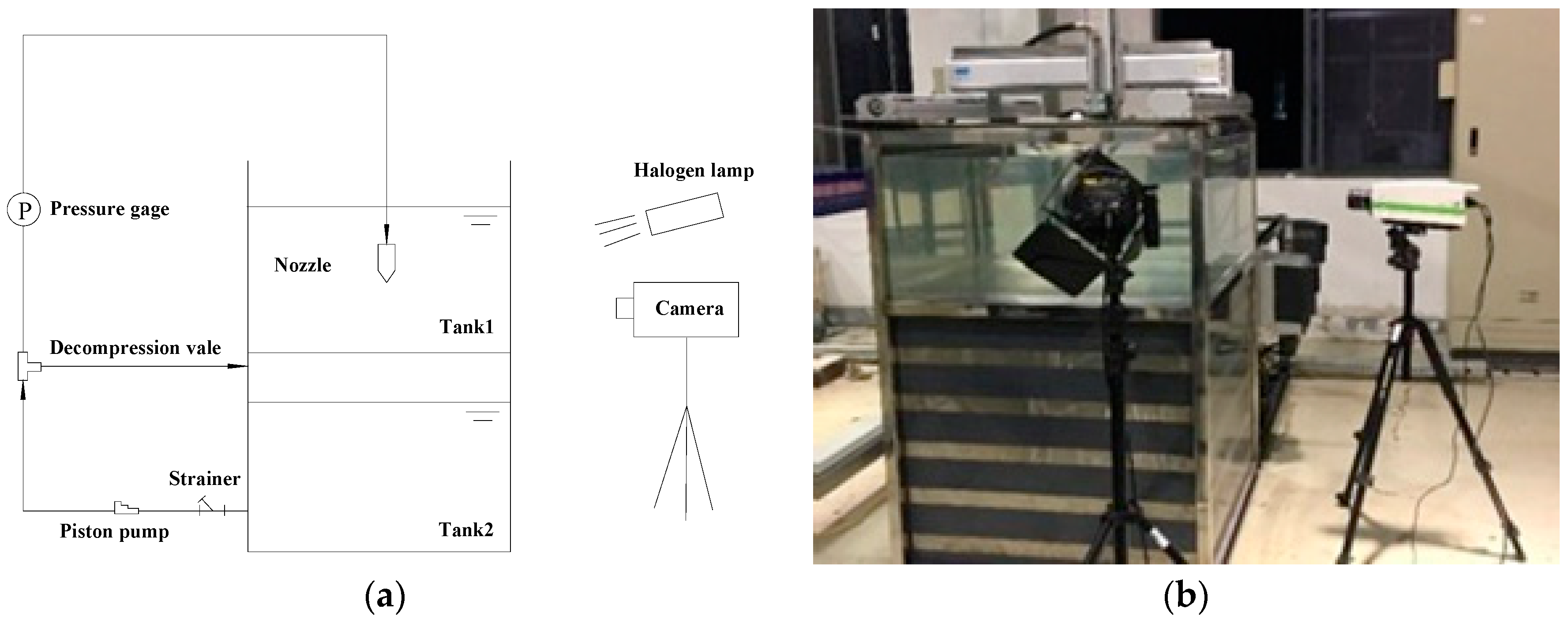
Figure 2.
Schematic diagram of the nozzle.

Figure 3.
Nozzles used in experiments.
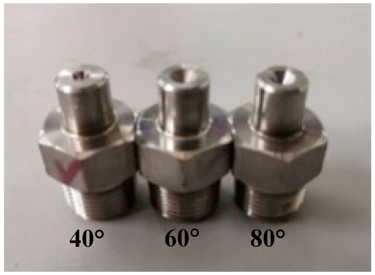
Figure 4.
Structure mesh of the submerged jet domain.

Figure 5.
Discharge coefficient predicted by CFD and tested by experiment.
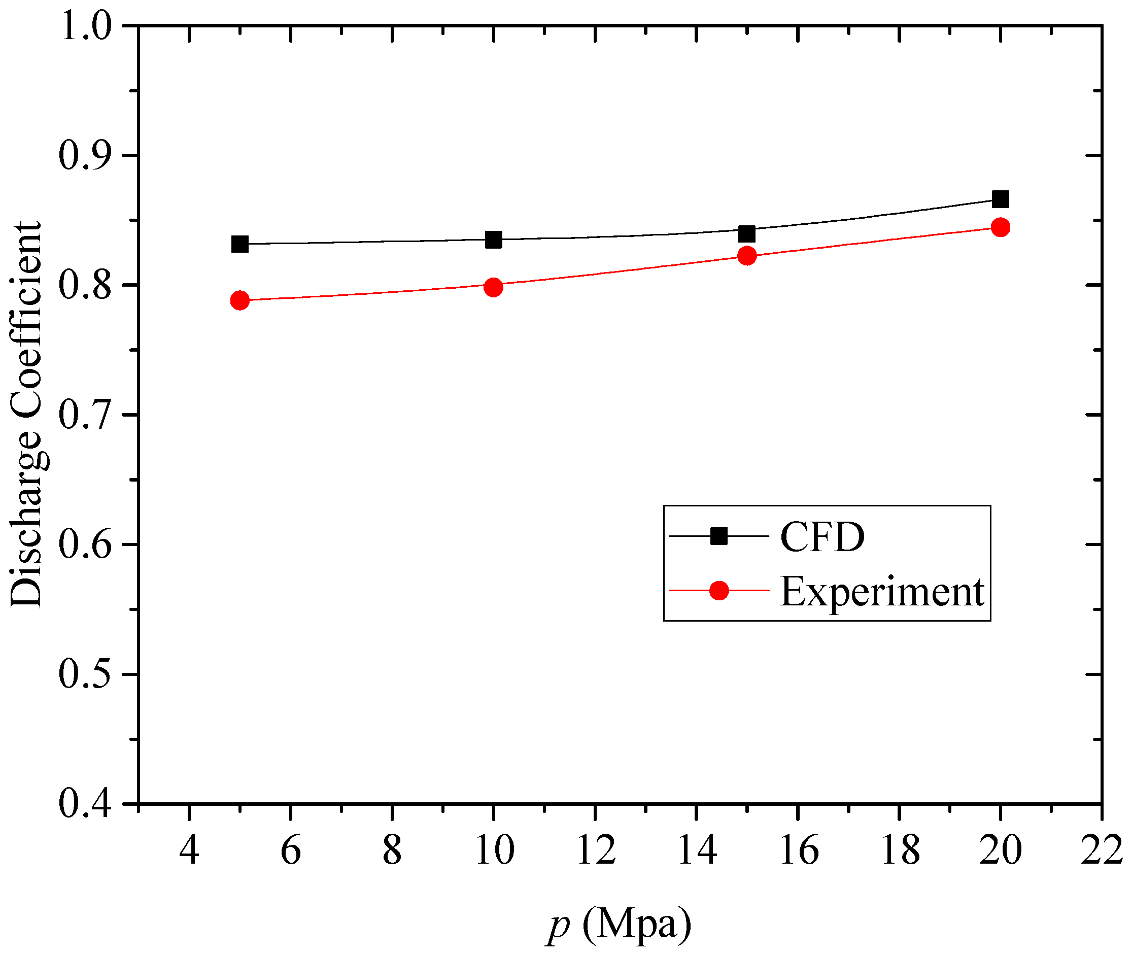
Figure 6.
Vapor volume fraction distribution of the submerged cavitation jet. (a) ZGB model, (b) current cavitation model, (c) experimental image
Figure 6.
Vapor volume fraction distribution of the submerged cavitation jet. (a) ZGB model, (b) current cavitation model, (c) experimental image

Figure 7.
Vapor volume fraction distribution of the submerged cavitation jet by experiment. (a) t = t0, (b) t = t0 + 250 μs, (c)t = t0 + 500 μs, (d)t = t0 + 750 μs, (e)t = t0 + 1000 μs, (f)t = t0 + 1250 μs.
Figure 7.
Vapor volume fraction distribution of the submerged cavitation jet by experiment. (a) t = t0, (b) t = t0 + 250 μs, (c)t = t0 + 500 μs, (d)t = t0 + 750 μs, (e)t = t0 + 1000 μs, (f)t = t0 + 1250 μs.

Figure 8.
Vapor volume fraction distribution of the submerged cavitation jet by CFD. (a) t = t0, (b) t =t0 + 250 μs, (c)t = t0 + 500 μs, (d)t = t0 + 750 μs, (e)t = t0 + 1000 μs, (f)t = t0 + 1250 μs.
Figure 8.
Vapor volume fraction distribution of the submerged cavitation jet by CFD. (a) t = t0, (b) t =t0 + 250 μs, (c)t = t0 + 500 μs, (d)t = t0 + 750 μs, (e)t = t0 + 1000 μs, (f)t = t0 + 1250 μs.

Figure 9.
Time-averaged vapor volume fraction of submerged jet from nozzle with different divergent angles. (a) 40° nozzle, (b) 60° nozzle, (c) 80° nozzle.
Figure 9.
Time-averaged vapor volume fraction of submerged jet from nozzle with different divergent angles. (a) 40° nozzle, (b) 60° nozzle, (c) 80° nozzle.

Figure 10.
Vapor volume fraction from a nozzle with different divergent angles. (a) 40° nozzle (b) 60° nozzle (c) 80° nozzle.
Figure 10.
Vapor volume fraction from a nozzle with different divergent angles. (a) 40° nozzle (b) 60° nozzle (c) 80° nozzle.

Figure 11.
Velocity profiles at different position downstream of nozzle exits. (a) 40° Original (b) 60° Original (c) 80° Original (d) 40° normalized (e) 60° normalized (f) 80° normalized.
Figure 11.
Velocity profiles at different position downstream of nozzle exits. (a) 40° Original (b) 60° Original (c) 80° Original (d) 40° normalized (e) 60° normalized (f) 80° normalized.
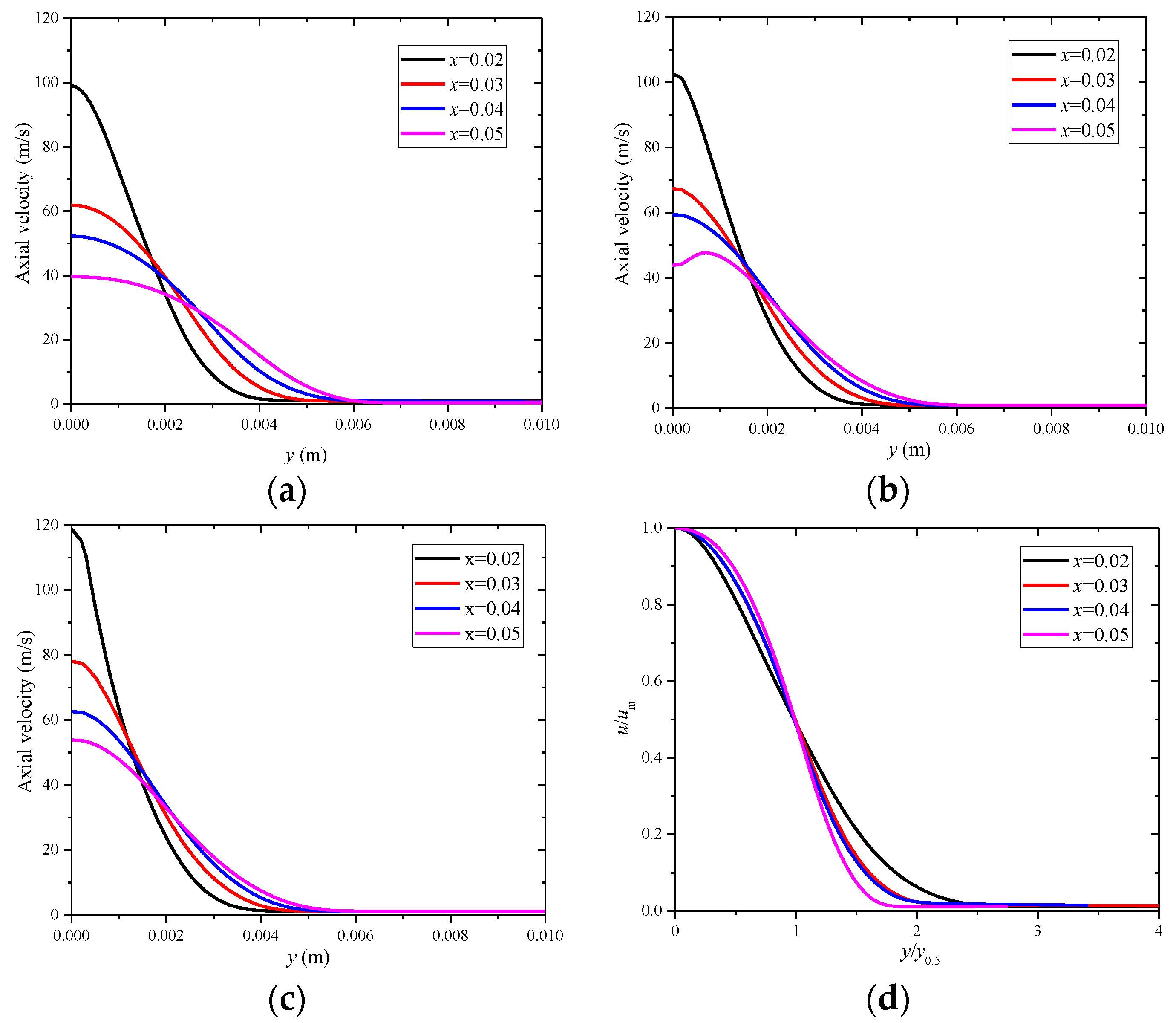

Figure 12.
Photograph of the aluminum surface after cavitation jet impingement using different nozzles with optimal distance: (a) p = 20 Mpa, s = 66 mm, α = 40°, t = 60 min; (b) p = 20 Mpa, s = 72 mm, α = 60°, t = 60 min; (c) p = 20 Mpa, s = 66 mm, α = 80°, t = 60 min.
Figure 12.
Photograph of the aluminum surface after cavitation jet impingement using different nozzles with optimal distance: (a) p = 20 Mpa, s = 66 mm, α = 40°, t = 60 min; (b) p = 20 Mpa, s = 72 mm, α = 60°, t = 60 min; (c) p = 20 Mpa, s = 66 mm, α = 80°, t = 60 min.
Figure 13.
Mass loss of the aluminum with different impingement times under the optimal distance. (a) 40° divergent angle (b) 60° divergent angle (c) 80° divergent angle.
Figure 13.
Mass loss of the aluminum with different impingement times under the optimal distance. (a) 40° divergent angle (b) 60° divergent angle (c) 80° divergent angle.


Table 1.
Factor level.
| Number | A L2 (mm) | B d (mm) | C L3 (mm) | D β (°) |
|---|---|---|---|---|
| 1 | 2 | 0.5 | 2 | 40 |
| 2 | 4 | 1.0 | 4 | 60 |
| 3 | 6 | 1.5 | 6 | 80 |
Table 2.
Orthogonal test schemes.
| Number | A | B | C | D |
|---|---|---|---|---|
| 1 | 2 | 0.5 | 2 | 40 |
| 2 | 2 | 1.0 | 4 | 60 |
| 3 | 2 | 1.5 | 6 | 80 |
| 4 | 4 | 0.5 | 4 | 80 |
| 5 | 4 | 1.0 | 6 | 40 |
| 6 | 4 | 1.5 | 2 | 60 |
| 7 | 6 | 0.5 | 6 | 60 |
| 8 | 6 | 1.0 | 2 | 80 |
| 9 | 6 | 1.5 | 4 | 40 |
Table 3.
Orthogonal calculation result.
| Number | 1 | 2 | 3 | 4 | 5 | 6 | 7 | 8 | 9 |
|---|---|---|---|---|---|---|---|---|---|
| VOF | 0.039 | 0.049 | 0.091 | 0.023 | 0.069 | 0.199 | 0.019 | 0.064 | 0.179 |
Table 4.
Range analysis of vapor volume fraction.
| Number | A | B | C | D |
|---|---|---|---|---|
| K1 | 1.027146 | 0.264775 | 1.071998 | 1.169487 |
| K2 | 1.058102 | 1.089607 | 0.96127 | 0.953527 |
| K3 | 0.979006 | 1.709872 | 1.030986 | 0.94124 |
| k1 | 0.342382 | 0.088258 | 0.357333 | 0.389829 |
| k2 | 0.352701 | 0.363202 | 0.320423 | 0.317842 |
| k3 | 0.326335 | 0.569957 | 0.343662 | 0.313747 |
| R | 0.026365 | 0.481699 | 0.036909 | 0.076082 |
© 2019 by the authors. Licensee MDPI, Basel, Switzerland. This article is an open access article distributed under the terms and conditions of the Creative Commons Attribution (CC BY) license (http://creativecommons.org/licenses/by/4.0/).
Share and Cite
MDPI and ACS Style
Yang, Y.; Li, W.; Shi, W.; Zhang, W.; A. El-Emam, M. Numerical Investigation of a High-Pressure Submerged Jet Using a Cavitation Model Considering Effects of Shear Stress. Processes 2019, 7, 541. https://doi.org/10.3390/pr7080541
AMA Style
Yang Y, Li W, Shi W, Zhang W, A. El-Emam M. Numerical Investigation of a High-Pressure Submerged Jet Using a Cavitation Model Considering Effects of Shear Stress. Processes. 2019; 7(8):541. https://doi.org/10.3390/pr7080541
Chicago/Turabian StyleYang, Yongfei, Wei Li, Weidong Shi, Wenquan Zhang, and Mahmoud A. El-Emam. 2019. "Numerical Investigation of a High-Pressure Submerged Jet Using a Cavitation Model Considering Effects of Shear Stress" Processes 7, no. 8: 541. https://doi.org/10.3390/pr7080541
Note that from the first issue of 2016, this journal uses article numbers instead of page numbers. See further details here.