High Pressure Injection of Chemicals in a Gravel Beach
by
 ,
,
Xiaolong Geng
1, 
Ali Abdollahi-Nasab
1,
Chunjiang An
2,
Zhi Chen
2,
Kenneth Lee
3 and
Michel C. Boufadel
1,* 1
Center for Natural Resources, Department of Civil and Environmental Engineering, Newark College of Engineering, New Jersey Institute of Technology, Newark, NJ 07102, USA
2
Department of Building, Civil and Environmental Engineering, Concordia University, Montreal, QC H4B 1R6, Canada
3
Department of Fisheries and Oceans, Dartmouth, NS B2Y 4A2, Canada
*
Author to whom correspondence should be addressed.
Processes 2019, 7(8), 525; https://doi.org/10.3390/pr7080525
Submission received: 19 June 2019
/
Revised: 18 July 2019
/
Accepted: 5 August 2019
/
Published: 8 August 2019
(This article belongs to the Special Issue Water Quality Modelling)
Abstract
:The remediation of beaches contaminated with oil includes the application of surfactants and/or the application of amendments to enhance oil biodegradation (i.e., bioremediation). This study focused on evaluating the practicability of the high pressure injection (HPI) of dissolved chemicals into the subsurface of a lentic Alaskan beach subjected to a 5 m tidal range. A conservative tracer, lithium, in a lithium bromide (LiBr) solution, was injected into the beach at 1.0 m depth near the mid-tide line. The flow rate was varied between 1.0 and 1.5 L/min, and the resulting injection pressure varied between 3 m and 6 m of water. The concentration of the injected tracer was measured from four surrounding monitoring wells at multiple depths. The HPI associated with a flow rate of 1.5 L/min resulted in a Darcy flux in the cross-shore direction at 1.15 × 10⁻⁵ m/s compared to that of 7.5 × 10⁻⁶ m/s under normal conditions. The HPI, thus, enhanced the hydraulic conveyance of the beach. The results revealed that the tracer plume dispersed an area of ~12 m2 within 24 h. These results suggest that deep injection of solutions into a gravel beach is a viable approach for remediating beaches.
1. Introduction
The 1989 Exxon Valdez oil spill in Prince William Sound (PWS) released around 37,000 metric tons of Alaskna North Slope crude oil onto the water. The spill reached 750 km to the southwest Deepthike, et al. [1], and polluted around 2000 km of shorelines in the Gulf of Alaska. Short, et al. [2,3] estimated that between 60 and 100 tons of oil still persist in many PWS beaches initially polluted with Exxon Valdez oil. The evidence of oil persistence in these beaches was also reported in various studies [4,5,6]. The persistent oil contains a considerable portion of polycyclic aromatic hydrocarbons (PAH), which are known to cause adverse ecological impact on wildlife upon exposure. Bodkin, et al. [7] reported that the increase in sea otter subpopulation was not at the expected rate in the heavily oiled northern Knight Island (NKI) area of PWS. Esler, et al. [8] reported that following the Exxon Valdez oil spill, the winter mortality of harlequin ducks in the NKI area and adjacent oiled areas of western Green Island and mainland between Crafton Island and Foul Bay increased more than expected. Techniques dealing with oil entrapped in beaches range from mechanical removal of contaminated sediments [9], to applying surface washing agents [10,11], and finally to in situ bioremediation [12,13,14]. The advantage of the latter technique, if applied onto the beach surface, is that it does not displace any of beach sediments or oil; it simply relies on delivery of needed chemicals (e.g., nutrients and dissolved oxygen) to the oil-contaminated zone [15]. However, the method could require major installations on gravel beaches, as was the case during the bioremediation of the Exxon Valdez oil spill [13]
The deficiency of nutrients (e.g., nitrate and phosphate) on these beaches was reported early during clean-up of the spill (from 1989 through 1992), due to which around 55 tons of nutrients have been applied on beaches of PWS [12]. Boufadel, et al. [16] demonstrated that the low oxygen concentration was a major cause for the negligible biodegradation of the oil. Short, et al. [2] estimated that the biodegradation rate of the oil was less than 4% per year.
Boufadel and Bobo [17], henceforth, BB2011, explored delivering nutrients and oxygen deep into the beach using high pressure injection (HPI) of solutions, and they used solutions of lithium bromide, where lithium was the conservative tracer, as the background bromide concentration (in seawater) is large. Deep injection of chemicals into aquifers is a common technique, but not much has been done in beaches.
Kloppmann, et al. [18] performed a 38-d injection test with Bromide, Boron and Lithium isotopes in a sandy aquifer to evaluate the transport dynamics of emerging chemical pollutants. Liu, et al. [19] conducted a Single-Well Injection-Withdrawal (SWIW) bromide tracer experiment to examine transport behavior at the Macrodispersion Experiment (MADE) site on Columbus Air Force Base in Mississippi. Damgaard, et al. [20] performed enhanced reductive dechlorination (ERD) by injecting molasses and dechlorinating bacteria into a clay till site contaminated with chlorinated ethenes. Most recently, Watson, et al. [21] conducted an injection test in an unconfined aquifer to assess the capacity of one-time emulsified vegetable oil (EVO) to maintain bioreduction of uranium in a highly permeable gravel layer.
If surfactant application or bioremediation were to be adopted on beaches, it would be during the summer, as winter temperatures are not conducive for oil biodegradation, and there is a possibility that the delivery will be conducted over multiple years, because one summer might not be sufficient for achieving the desired level of oil translocation and/or biodegradation. One of the crucial questions is whether the beach properties change drastically from year to year, requiring very different values of design parameters, such as flow rate or requiring even different designs. The tracer study of BB2011 was conducted in the Summer of 2009, and we report herein a similar tracer study conducted a year later, in the Summer of 2010. Our hypothesis was that the beach properties had not changed considerably over the year.
This study focused on a beach located on Eleanor Island, labeled EL056C (147°34′17.42″ W, 60°33′45.57″ N). The studied beach was 40 m wide in the along-shore direction and 50 m long in the across-shore direction (Figure 1). The beach was severely contaminated by the Exxon Valdez oil spill, and extensive treatment was implemented on it [5]. The oil residuals were considered to persist in this beach [3]. According to recent investigations, oil is located on the right (looking landward) side of the beach between the mid-tide level and the low-tide level, while the left side of the beach is clean [6,16]. Measurements in this beach at depths ranging from 0.50 to 0.80 m confirmed the lack of nutrients and the existence of near-anoxic conditions [16].
2. Methods and Materials
2.1. Field Setup
The depth of the bedrock in the beach was estimated at 2.0 to 3.0 m. Five pits were excavated in the beach (Figure 1a,b). One was used to place the injection well, and the remaining four surrounded the injection well and included the observation wells, labeled as “InjSea,” “InjLand,” “InjLeft,” and “InjRight,” which represented the locations of sea side, land side, left side, and right side of the tracer injection well, respectively (Figure 1b). A PVC pipe, a multiport sampling well, and two sampling boxes (SBs) were deployed in each pit. The PVC pipe (I.D. = 1″) was slotted across over its entire length to allow pore water passage. A pressure transducer (Mini-Diver, dataLogger) was deployed at the bottom of the PVC pipe to measure the water pressure at 10-min intervals. An air-pressure sensor (BaroLogger, DL-500, Schlumberger, Houston, TX) was used to monitor barometric pressure. The groundwater table’s pressure was determined by subtracting the barometric pressure from the water pressure recorded from the pressure transducers. The multiport sampling wells contained sampling ports (SPs) at intervals of 0.23 m, which were labeled A, B, C, and D from the bottom up. Water samples were collected at the top of the pipe from a tygon tube connected to each port location through a tube. The sampling box (SB) was made of two perforated concentric cylinders between which uniform sands were filled [17]. The depths of SPs and SBs for the observation wells are shown in Table 1.
2.2. HPI Conservative Tracer
Lithium as technical grade anhydrous (ReagentPlus grade, assay >99%) lithium bromide (LiBr) was selected as the conservative tracer for our study. It was successfully used in previous tracer studies for aquifer beach systems [22]. The design of tracer injection was to maintain a constant concentration of 100 mg/L for 33 h and then suddenly reduce it to 0.0 mg/L by pumping only seawater in order to analyze the flushing process of the tracer. The concentration of lithium was determined by analysis using atomic absorption spectroscopy with an air-acetylene flame at 670.8 nm. The pressure used for the tracer injection was adjusted by the flow rate pumped through the injection well.
The operational pressure and associated flow rate injected into the beach had to be less than the blow-out values (i.e., maximum), which were 3.0 L/min for the flow and 196 kPa for the pressure. The blow-out values for the design were determined by BB2011 through injection of pressurized seawater to assess the beach capacity until failure or fracturing of soil. Hence, using a flow rate higher than that of BB2011 would have led to fractures with higher permeability and eventually forced the system to rapidly escalate into a blow-out either in the higher layer or in the surface of the beach.
The injection lasted for 44 h, from 12:00, 20 August, 2010—08:00, 22 August, 2010. The flow rate was elevated from 1.0 to 1.5 L/min and the corresponding pressure fluctuated between 3 m (29 kPa) and 6 m (58 kPa). Measurements from the sampling wells began once the injection started, and lasted for 53 h (i.e., 9 h after the injection had stopped). The sampling was dependent on several factors, such as logistics, human power, and the tide level. Further technical details on the used instruments and sampling wells can be found in BB2011.
3. Results
The starting time of the experiment, 12:00, 20 August, 2010, was set as time t = 0 for all the figures. We first report the results of the total head variation with time, followed by those of the concentration. Figure 2 shows variation of the flow rate and total head at the well during the injection period. The flow rate was 1.0 L/min for 20 h during which the variation of pressure head was mainly controlled by tide fluctuations. At t = 10 h, for instance, the pressure head increased to 5.0 m following the high tide which reached 4.5 m. At t = 20 h, the injection rate was elevated to 1.5 L/min and remained constant until the end of the injection process. At t = 25 h, the injection started to put a higher pressure on the sediment than that from tide. The increase in the flow rate increased the pressure head to 6 m at high tide (t = 35 h) compared to that of 5 m for the same tide and when the flow rate was 1.0 L/min (t = 10 h).
Due to logistical constraints, it was not feasible to maintain the concentration at 100 mg/L. Our field experiments recorded that eight measurements of the concentration in the tanks had an average concentration of 88 mg/L with a standard deviation of 14 mg/L (Figure 3). The variance of the concentration was sufficiently small compared to the change of concentration from 100 to 0.0 mg/L for overall experimental design. Herein, 10% of the maximum tracer concentration was used to delineate the ‘edge of the plume.’ This is a subjective criterion, but it was needed in the absence of a numerical model. A justification for it was provided by BB2011, Boufadel and Bobo [17], and publications therein. With a maximum of 88 mg/L, values larger than 8.8 mg/L were viewed as part of the injected plume, whereas values smaller than 8.8 mg/L were assumed to be “not effective” for remediating the beach. The lithium concentration measured from all the sampling wells is reported in Table S1. Figure 4 shows the temporal change of the lithium concentration at various depths during the injection process at well InjSea. The concentration reached its peak of 60 mg/L at SB Shallow, 80 mg/L at SP_A, and 95 mg/L at SB Deep at t = 33 h. The continuous increase in concentration at all the sampling locations before t = 33 h reflects the lithium injection process. At t ≈ 53 h (i.e., the last sample event), the concentration decreased in almost all the sampling locations to 20 mg/L because the injected concentration decreased from 100 mg/L (88 mg/L ± 14 mg/L) to 0.0 mg/L at t = 33 h. The travel time for the injected water to reach the different sampling depths of well InjSea varied between 6 h for SP_A, and 20 h for SB Deep and SB Shallow (Figure 4). This difference in travel time is most likely due to the local heterogeneity of the beach. From this range of time of arrival, and based on the distance between the injection well and well InjSea (Figure 1a), one deduces that the travel speed of the tracer plume in the seaward direction was between 3 m/d and 10 m/d. Note that this estimation for organic compounds would be affected by interaction with soil and sand through adsorption and desorption processes.
Figure 5 shows that the tracer reached 10% (8.8 mg/L) of the maximum injected concentration in well InjLand at t = 24 h. Therefore, the landward transit speed of the plume was approximately 1.6 m/d, which was estimated by the distance between well Inj and well InjLand divided by arrival time of the tracer at Well InjLand. Note that the injection was implemented at time t = 0. The concentration at SB Shallow, first rose to ~10 mg/L at t = 27 h, and then dropped to ~2.0 mg/L at t = 53 h. In contrast, the concentration at SP_A and SB Deep, first increased to 5 mg/L at t = 27 h, and then decreased to 2 mg/L at t = 53 h. This was because the injection concentration decreased from 88 mg/L to 0.0 mg/L at t = 33 h. In addition, Figure 5 indicates a considerable depth of 0.74 m that the tracer reached at landward of the injection well. That suggests that these injection techniques should sustain such a concentration landward of the applications, based on the mass conservation principle.
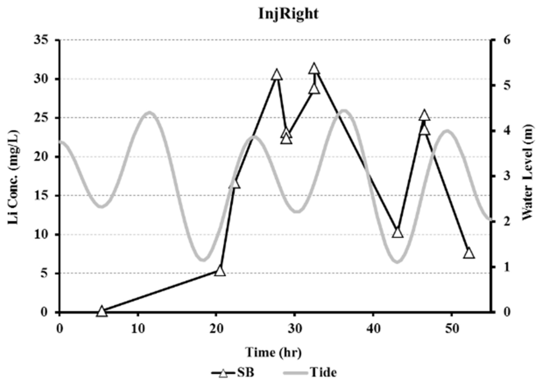
The tracer movement was also quantified between wells InjLeft and InjRight, representing the movement in the along-shore direction. The objective was to isolate the effect of tide which caused cross-shore transport, but not in the along-shore direction [6]. Figure 6 reports that prior to t = 20 h, the concentration in the sampling sensors at different locations was less than 2 mg/L, which is too small to represent the tracer plume. However, it indicates a certain mobility of the tracer after the pumping started. The concentrations first reached the peaks at t = 27 h for all the sampling locations, which were 34 mg/L, 47 mg/L, 20 mg/L, and 25 mg/L at SP_A, SP_B, SB Deep, and SB Shallow, respectively. Afterward, it dropped to less than 10 mg/L, which is because of the decrease in the source lithium concentration from ~88 mg/L to 0.0 mg/L at t = 33 h. Our results indicate that the transit time of the tracer plume to well InjLeft was between 20 h and 30 h, resulting in an average long-shore migration speed of ~2.0 m/d. In the Well InjRight, only one SB was available at 0.52 m below the surface, and using arguments adopted for Figure 6 and Figure 7 indicates that the transit speed of the tracer plume in the long-shore right direction was ~1.8 m/d.
Figure 8 shows the migration of the injected plume as percentage of the injection concentration. The plume contours were obtained as follows: Temporal variations of the maximum concentrations at each monitoring well from all SPs and SBs were plotted. Focus was placed on t = 6.5 h and t = 21 h, because many measurements occurred around that time due to logistics (access and tide). Linear interpolation was conducted from the time series, and then, the values were projected on the corresponding well locations. Then, the concentration contours at t = 6.5 h and 21 h were obtained using SURFER software.
The upper panel of Figure 8 indicates that within 6 h from injection, the plume occupied a considerable area (12 m2). One can also note that there was no significant change in the spreading of the plume at t = 21 h, notably in the landward direction (Figure 8, lower panel). This indicates that the spreading rate of the plume was high initially but the subsequent rate dropped fast. This is most likely due to: (1) Increased interaction with “clean” water as the tracer moved away from the injection point; and (2) the radial geometry of the plume as a result of the injection led to a faster decrease in tracer mass per unit peripheral length.
4. Discussion
The temporal variation of the concentrations, measured in four monitoring wells around the injection well, portrayed the tracer migration in the beach. The concentrations in the monitoring wells first reached their peaks within 35 h due to the tracer injection and then dropped when the tracer concentration was switched from 88 mg/L into 0.0 mg/L at time t = 33 h. The concentration peaks measured in all the monitoring wells were above 10% of the average injected concentration (88 mg/L). This indicates that the design of a HPI system was feasible to deliver dissolved chemicals, such as nutrients and oxygen, to the oiled zone of Beach EL056C. The measurements also showed that the impact of tide fluctuation was negligible on the temporal variation of the tracer concentrations in almost all the monitoring wells. This result was consistent with the investigation carried out by BB2011. The beach has a two-layered hydraulic structure: A surface layer with high permeability, underlain by a low-permeability lower layer. The oil was trapped in the lower layer of the beach with the low hydraulic conductivity of 5 × 10⁻⁵ m/s [6]. The low permeability was limiting the hydraulic conveyance of the oiled zone, and in addition to the near-anoxic condition, pointed out the low seawater–groundwater mixing in the lower layer of the beach. It could, to some extent, support the feasibility of HPI system for delivering either surfactants or nutrients (in case of bioremediation) to the oil region, as the dissolved chemicals would not be diluted by seawater when the injection is conducted in the lower layer of the beach.
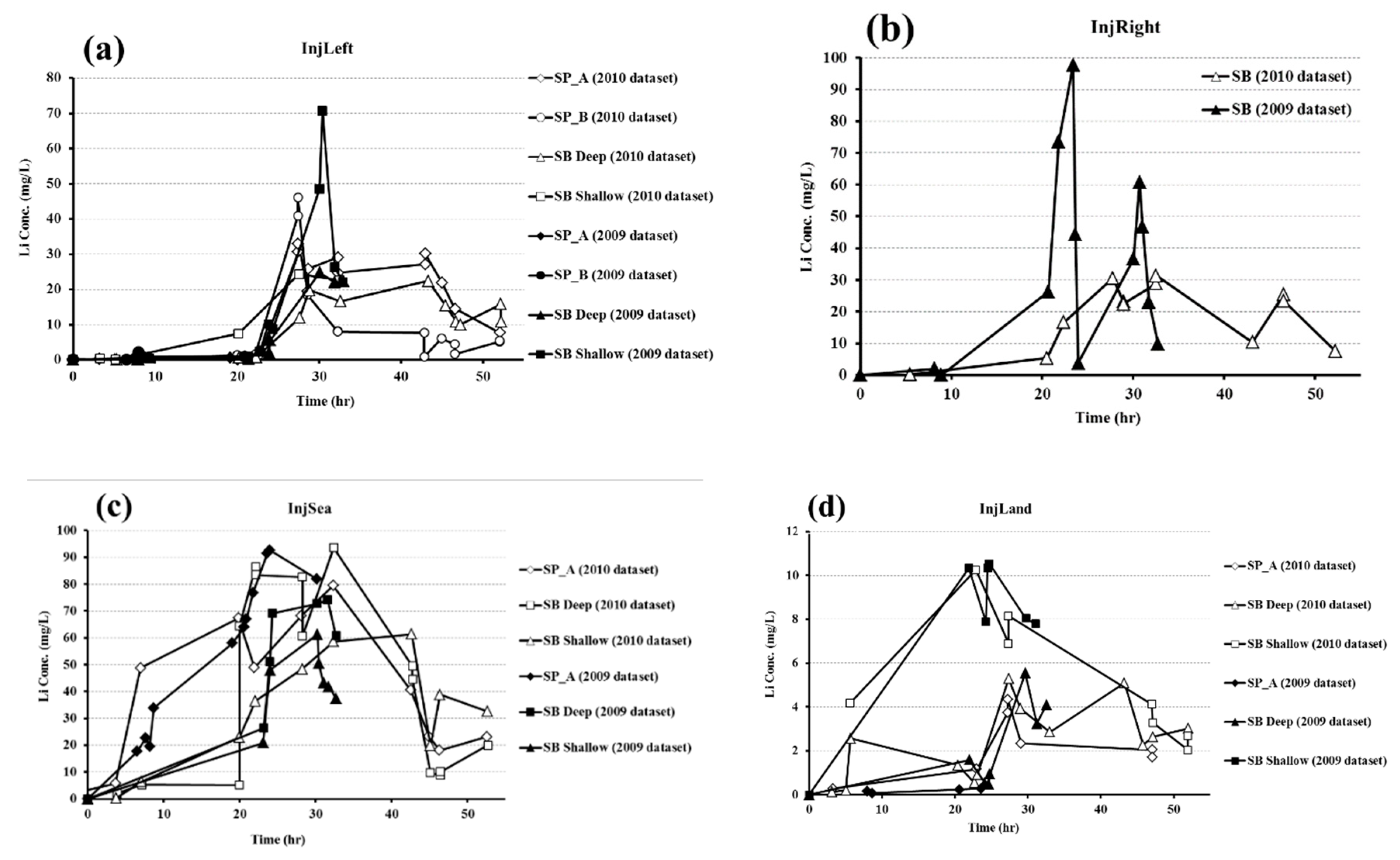
The observed data were also comparable to those of BB2011 that were obtained a year earlier (2009) on the same beach using similar injection procedures and experimental setup (Figure 9). The good agreement shows that the general dynamic behavior of the tracer and its travel time in the 2010 dataset were consistent with those measured in 2009 (Figure 9). However, the concentrations in the along-shore direction were significantly different at the shallow sampling locations (Figure 9a). In the BB2011 dataset, the concentration at SB Shallow of well InjLeft reached its peak value of 70 mg/L at t = 30 h, whereas in 2010 the concentration reached a much smaller peak value 25 mg/L at a comparable time (t = 27 h). In contrast, there was almost no concentration difference at SB Deep of well InjLeft. A similar behavior was noted in well InjRight, in which the concentration at SB reached its peak value of 98 mg/L at t = 23 h in 2009 and 30 mg/L at t = 27 h in 2010 (Figure 9b). This difference is most likely due to the local heterogeneity of the beach, which could result in different spreading rates of the tracer. In contrast to those in the along-shore direction, the concentrations at the sampling locations in the cross-shore direction did not show a significant difference between 2009 and 2010 (Figure 9c,d). This is probably because the large hydraulic gradient caused by tide action (5 m tide range) diminished the effect of local heterogeneity on tracer movement. One notes that even though these uncertainties impacted the concentration at certain shallow sampling locations in 2010, the peak concentration in all monitored wells was still above 10% of the maximum, which we used to delineate the plume edge. The results, thus, strengthen the feasibility of delivering dissolved chemicals by HPI to the oil-contaminated zone.
The comparison of water heads between this dataset and the one carried out by BB2011 (not shown in this paper for brevity) shows that when the flow rate is equal to 1.0 L/min and the well was submerged by high tide, the water head was almost similar to that of the tide level. Therefore, one can conclude that the buildup pressure of injection would be negligible in comparison to tidal effect.
The magnitude of the hydraulic gradient (HG) of the beach, negative in the seaward direction and positive in the landward one, decreased during high tide and increased during low tide. The cross-shore distance of intertidal zone, used to estimate the hydraulic gradient, was approximately 36 m and the tidal range was around 5.5 m. Therefore, the estimated hydraulic gradient without injection ranged from 0 at high tide to −0.16 at low tide. With injection, the cross-shore distance between the injection well and the low tide (20 m) was used to calculate the HG. The flow rate of 1 L/min, as reported earlier, had minimal impact on the water head and, hence, on the HG. When the flow rate increased to 1.5 L/min and during high tide, the water head increased by 1.5 m above the tide level and the estimated HG was −0.075. For the same flow (1.5 L/min) and during low tide, the water head increased by 4 m above the tide level which resulted in a HG equal to −0.23. The hydraulic conductivity (i.e., K) in the oil-trapped layer (i.e., the lower layer of the beach) was estimated to be 5.0 × 10⁻⁵ m/s [6]. Therefore, the HPI associated with a flow rate of 1.5 L/min resulted in a maximum Darcy flux (q = −K × (ΔH/L)) in the cross-shore direction at 1.15 × 10⁻⁵ m/s (i.e., 5.0 × 10⁻⁵ m/s × 0.23), compared to that of 8.0 × 10⁻⁶ m/s (i.e., 5.0 × 10⁻⁵ m/s × 0.16) under normal conditions. The results suggest that HPI, under appropriate flow rates, enhanced the hydraulic conveyance of the beach, which is an indicator implying that the HPI of chemicals (e.g., nutrients and dissolved oxygen) would enhance oil biodegradation and/or the HPI of surfactants would allow dislodgement of entrapped oil.
The diameter of the influence of the well from HPI was found to be approximately 3.0 m (Figure 8), which is consistent with the results obtained by BB2011. The migration diameter of both datasets confirms that delivery of chemicals via injection is logistically practical. In terms of the findings on this beach, the estimated oil-contaminated area was ~25 m2. Therefore, two to three injection wells would be needed for complete coverage of oil-contaminated zone by the injected chemicals in order to achieve an effective remediation. In order to minimize the impact of precipitation, setting injection wells along cross-shore directions is recommended.
5. Conclusions
The remediation of beaches contaminated with oil includes the application of surfactants and/or the application of amendments to enhance oil biodegradation (i.e., bioremediation). This study focused on evaluating the feasibility of the high pressure injection (HPI) of dissolved chemicals (e.g., nutrients and dissolved oxygen) into the subsurface of a lentic Alaskan beach subjected to a 5 m tidal range, and to compare the results to those obtained the prior year. The hypothesis was that beach hydrogeology did not change within one year. A conservative tracer, lithium, in a lithium bromide (LiBr) solution, was injected into the beach at about 1-m deep location near the mid-tide line. The flow rate was varied between 1.0 and 1.5 L/min, and the resulting injection pressure varied between 3 m and 6 m of water. The concentration of injected tracer was measured at different depths from four surrounding monitoring wells. The measurement results agreed with the prior study. The HPI associated with a flow rate of 1.5 L/min resulted in a Darcy flux in the cross-shore direction, at 1.15 × 10⁻⁵ m/s compared to that of 7.5 × 10⁻⁶ m/s under normal conditions, an increase of 50% in the water velocity. The HPI, thus, enhanced the hydraulic conveyance of the beach. The results revealed that the tracer plume spread over an area of 12 m2 within 24 h. These results suggest that deep injection of solutions into a gravel beach is a viable approach for remediating beaches.
Supplementary Materials
The supplementary materials are available online at https://www.mdpi.com/2227-9717/7/8/525/s1.
Author Contributions
M.C.B. conceived and designed the experiments; A.A.N. and X.G. performed the experiments; M.C.B. and X.G. analyzed the data and wrote the paper. K.L., C.A., and Z.C. contributed the conception of the work and to improving the overall quality of the work and manuscript.
Funding
This research received no external funding.
Acknowledgments
This research was made possible, in part, by MPRI Project 2.01 from the Multi Partner Research Initiative Project Oil Translocation from the Department of Fisheries and Oceans, Canada. However, it does not necessarily reflect the views of the funding entity; no official endorsement should be inferred.
Conflicts of Interest
The authors declare no conflict of interest.
References
- Deepthike, H.U.; Tecon, R.; Kooten, G.v.; Meer, J.R.v.d.; Harms, H.; Wells, M.; Short, J. Unlike PAHs from Exxon Valdez crude oil, PAHs from Gulf of Alaska coals are not readily bioavailable. Environ. Sci. Technol. 2009, 43, 5864–5870. [Google Scholar]
- Short, J.; Maselko, J.; Lindeberg, M.; Harris, P.; Rice, S. Vertical distribution and probability of encountering intertidal Exxon Valdez oil on shorelines of three embayments within Prince William Sound, Alaska. Environ. Sci. Technol. 2006, 40, 3723–3729. [Google Scholar] [CrossRef]
- Short, J.W.; Lindeberg, M.R.; Harris, P.M.; Maselko, J.M.; Pella, J.J.; Rice, S.D. Estimate of oil persisting on the beaches of Prince William Sound 12 years after the Exxon Valdez oil spill. Environ. Sci. Technol. 2004, 38, 19–25. [Google Scholar] [CrossRef]
- Irvine, G.V.; Mann, D.H.; Short, J.W. Persistence of 10-year old Exxon Valdez oil on Gulf of Alaska beaches: The importance of boulder-armoring. Mar. Pollut. Bull. 2006, 52, 1011–1022. [Google Scholar] [CrossRef] [PubMed]
- Taylor, E.; Reimer, D. Oil persistence on beaches in Prince William Sound—A review of SCAT surveys conducted from 1989 to 2002. Mar. Pollut. Bull. 2008, 56, 458–474. [Google Scholar] [CrossRef] [PubMed]
- Li, H.; Boufadel, M.C. Long-term persistence of oil from the Exxon Valdez spill in two-layer beaches. Nature Geosci. 2010, 3, 96–99. [Google Scholar] [CrossRef]
- Bodkin, J.L.; Ballachey, B.E.; Coletti, H.A.; Esslinger, G.G.; Kloecker, K.A.; Rice, S.D.; Reed, J.A.; Monson, D.H. Long-term effects of the ‘Exxon Valdez’ oil spill: Sea otter foraging in the intertidal as a pathway of exposure to lingering oil. Mar. Ecol. Prog. Ser. 2012, 447, 273–287. [Google Scholar] [CrossRef]
- Esler, D.; Bowman, T.D.; Trust, K.A.; Ballachey, B.E.; Dean, T.A.; Jewett, S.C.; O’Clair, C.E. Harlequin duck population recovery following the ‘Exxon Valdez’ oil spill: Progress, process and constraints. Mar. Ecol. Prog. Ser. 2002, 241, 271–286. [Google Scholar] [CrossRef]
- Owens, E.H.; Davis, I.A., Jr.; Michel, J.; Stritzke, K. Beach cleaning and the role of technical support in the 1993 tampa bay spill. In Proceedings of the 2005 International Oil Spill Conference, Miami Beach, FL, USA, 15–19 May 2005; pp. 566–583. [Google Scholar]
- Taylor, E.; Owens, E.H. Specialized mechanical equipment for shoreline cleanup. In Proceedings of the International Oil Spill Conference, Washington, DC, USA, 7–11 April 1997; pp. 79–87. [Google Scholar]
- Stegemeier, G. Improved Oil Recovery by Surfactant and Polymer Flooding; Shah, D.O., Schechter, R.S., Eds.; Academic Press: New York, NY, USA, 1977; Volume I. [Google Scholar]
- Bragg, J.R.; Prince, R.C.; Harner, E.J.; Atlas, R.M. Effectiveness of bioremediation for the Exxon Valdez oil spill. Nature 1994, 368, 413–418. [Google Scholar] [CrossRef]
- Boufadel, M.C.; Geng, X.; Short, J. Bioremediation of the Exxon Valdez oil in Prince William Sound beaches. Mar. Pollut. Bull. 2016. [Google Scholar] [CrossRef] [PubMed]
- Lee, K.; Tremblay, H. Bioremediation: Application of slow-release fertilizers on low energy shorelines. In Proceedings of the 1993 International Oil Spill Conference, Washington, DC, USA, 29 March–1 April 1993; pp. 449–454. [Google Scholar]
- Venosa, A.D.; Suidan, M.T.; Wrenn, B.A.; Strohmeier, K.L.; Haines, J.; Eberhart, B.L.; King, D.; Holder, E. Bioremediation of an experimental oil spill on the shoreline of Delaware Bay. Environ. Sci. Technol. 1996, 30, 1764–1775. [Google Scholar] [CrossRef]
- Boufadel, M.C.; Sharifi, Y.; Van Aken, B.; Wrenn, B.A.; Lee, K. Nutrient and Oxygen Concentrations within the Sediments of an Alaskan Beach Polluted with the Exxon Valdez Oil Spill. Environ. Sci. Technol. 2010, 44, 7418–7424. [Google Scholar] [CrossRef]
- Boufadel, M.C.; Bobo, A.M. Feasibility of high pressure injection of chemicals into the subsurface for the bioremediation of the exxon valdez oil. Ground Water Monit. Remediat. 2011, 31, 59–67. [Google Scholar] [CrossRef]
- Kloppmann, W.; Chikurel, H.; Picot, G.; Guttman, J.; Pettenati, M.; Aharoni, A.; Guerrot, C.; Millot, R.; Gaus, I.; Wintgens, T. B and Li isotopes as intrinsic tracers for injection tests in aquifer storage and recovery systems. Appl. Geochem. 2009, 24, 1214–1223. [Google Scholar] [CrossRef]
- Liu, G.; Zheng, C.; Tick, G.R.; Butler, J.J., Jr.; Gorelick, S.M. Relative importance of dispersion and rate-limited mass transfer in highly heterogeneous porous media: Analysis of a new tracer test at the Macrodispersion Experiment (MADE) site. Water Resour. Res. 2010, 46, W03524. [Google Scholar] [CrossRef]
- Damgaard, I.; Bjerg, P.L.; Jacobsen, C.S.; Tsitonaki, A.; Kerrn-Jespersen, H.; Broholm, M.M. Performance of Full-Scale Enhanced Reductive Dechlorination in Clay Till. Groundwater Monit. Remediat. 2013, 33, 48–61. [Google Scholar] [CrossRef]
- Watson, D.B.; Wu, W.; Mehlhorn, T.; Tang, G.; Earles, J.; Lowe, K.; Gihring, T.M.; Zhang, G.; Phillips, J.; Boyanov, M. In situ bioremediation of uranium with emulsified vegetable oil as the electron donor. Environ. Sci. Technol. 2013, 47, 6440–6448. [Google Scholar] [CrossRef] [PubMed]
- Wrenn, B.A.; Suidan, M.T.; Strohmeier, K.L.; Eberhart, B.L.; Wilson, G.J.; Venosa, A.D. Nutrient transport during bioremediation of contaminated beaches: Evaluation with lithium as a conservative tracer. Water Res. 1997, 31, 515–524. [Google Scholar] [CrossRef]
Figure 1.
(a) The injection well along with four surrounding sampling wells in the field. Note that the sea is to the left in this figure. (b) Top view showing the topographic contours of Beach EL056C. The injection well (labeled Inj) is at the approximate location x = 25 m, y = 28 m. It is surrounded by four observation wells: On the landward side (InjLand), on the seaward side (InjSea), on the left (InjLeft), and on the right (InjRight).

Figure 2.
Variation of the flow rate and pressure during tracer injection. The injection occurred until t = 44 h. The average injection concentration between 0.0 h and 33 h was 88 mg/L, after which it was reduced to 0.0 mg/L.
Figure 2.
Variation of the flow rate and pressure during tracer injection. The injection occurred until t = 44 h. The average injection concentration between 0.0 h and 33 h was 88 mg/L, after which it was reduced to 0.0 mg/L.

Figure 3.
Variation of injected concentration as a function of time at the injection well. The eight measurements of the concentration in the tanks had an average of 88 mg/L with a standard deviation of 14 mg/L.
Figure 3.
Variation of injected concentration as a function of time at the injection well. The eight measurements of the concentration in the tanks had an average of 88 mg/L with a standard deviation of 14 mg/L.

Figure 4.
Variation of the concentration at various vertical locations at InjSea, which was 2.5 m seaward of the injection well (Figure 1). The depth of each sampling Ports (SP) and sampling Box (SB) is reported in Table 1.

Figure 5.
Variation of the concentration at various vertical locations at InjLand, which was 1.6 m landward of the injection well. The depth of each SP and SB is reported in Table 1.
Figure 5.
Variation of the concentration at various vertical locations at InjLand, which was 1.6 m landward of the injection well. The depth of each SP and SB is reported in Table 1.

Figure 6.
Variation of the concentration at various vertical locations at InjLeft, which was 1.7 m landward of the injection well. The depth of each SP and SB is reported in Table 1.
Figure 6.
Variation of the concentration at various vertical locations at InjLeft, which was 1.7 m landward of the injection well. The depth of each SP and SB is reported in Table 1.

Figure 7.
Variation of the concentration at various vertical locations at InjRight, which was 1.5 m right (looking landward) of the injection well. Only one SB was placed at this location.
Figure 7.
Variation of the concentration at various vertical locations at InjRight, which was 1.5 m right (looking landward) of the injection well. Only one SB was placed at this location.

Figure 8.
Empirical contours of lithium concentration as a percentage of the maximum at two different times, 6.5 and 21 h. The injection point was at the approximate location x = 25 m, y = 28 m. The edge of the plume was delineated where the concentration was 10% of the maximum. The figure indicates that at t = 21 h, the injected plume occupied an approximate area of 12 m2.

Figure 9.
Comparison between the concentration values from the sampling wells, InjLeft (a), InjRight (b), InjSea (c), and InjLand (d), for the 2010 dataset and a dataset obtained in a prior year using similar experimental and injection procedures [17].
Figure 9.
Comparison between the concentration values from the sampling wells, InjLeft (a), InjRight (b), InjSea (c), and InjLand (d), for the 2010 dataset and a dataset obtained in a prior year using similar experimental and injection procedures [17].


Table 1.
Surface elevations and depths of sampling boxes (SBs) and sampling ports (SPs) from the surface for the corresponding well locations.
Table 1.
Surface elevations and depths of sampling boxes (SBs) and sampling ports (SPs) from the surface for the corresponding well locations.
| Location | Surface Elevation (m) | Depth of SP_A (m) | Depth of SP_B (m) | Depth of SB_Deep (m) | Depth of SB_SH (m) |
|---|---|---|---|---|---|
| InjLand | 3.66 | 0.54 | 0.35 | 0.74 | 0.40 |
| InjSea | 3.12 | 0.69 | 0.50 | 0.84 | 0.56 |
| InjLeft | 3.30 | 0.63 | 0.44 | 0.77 | 0.56 |
| InjRight | 3.30 | - | - | - | 0.52 |
© 2019 by the authors. Licensee MDPI, Basel, Switzerland. This article is an open access article distributed under the terms and conditions of the Creative Commons Attribution (CC BY) license (http://creativecommons.org/licenses/by/4.0/).
Share and Cite
MDPI and ACS Style
Geng, X.; Abdollahi-Nasab, A.; An, C.; Chen, Z.; Lee, K.; Boufadel, M.C. High Pressure Injection of Chemicals in a Gravel Beach. Processes 2019, 7, 525. https://doi.org/10.3390/pr7080525
AMA Style
Geng X, Abdollahi-Nasab A, An C, Chen Z, Lee K, Boufadel MC. High Pressure Injection of Chemicals in a Gravel Beach. Processes. 2019; 7(8):525. https://doi.org/10.3390/pr7080525
Chicago/Turabian StyleGeng, Xiaolong, Ali Abdollahi-Nasab, Chunjiang An, Zhi Chen, Kenneth Lee, and Michel C. Boufadel. 2019. "High Pressure Injection of Chemicals in a Gravel Beach" Processes 7, no. 8: 525. https://doi.org/10.3390/pr7080525
Note that from the first issue of 2016, this journal uses article numbers instead of page numbers. See further details here.