Measuring Efficiency of Generating Electric Processes

Abstract

Electric energy sources are the foundation for supporting for the industrialization and modernization; however, the processes of electricity generation increase CO₂ emissions. This study integrates the Holt–Winters model in number cruncher statistical system (NCSS) to estimate the forecasting data and the undesirable model in data envelopment analysis (DEA) to calculate the efficiency of electricity production in 14 countries all over the world from past to future. The Holt–Winters model is utilized to estimate the future; then, the actual and forecasting data are applied into the undesirable model to compute the performance. From the principle of an undesirable model, the study determines the input and output factors as follows nonrenewable and renewable fuels (inputs), electricity generation (desirable output), and CO₂ emissions (undesirable output). The empirical results exhibit efficient/inefficient terms over the period from 2011–2021 while converting these fuels into electricity energy and CO₂ emissions. The efficiency reveals the environmental effect level from the electricity generation. The analysis scores recommend a direction for improving the inefficient terms via the principle of inputs and undesirable outputs excess and desirable outputs shortfalls in an undesirable model.

1. Introduction

In recent years, the electricity industry has been extended to meet the demands of growth economic sustainably [1], which provides an energy source for lighting, heating, cooling, transportation, information exchange, i.e., electrical energy is derived from nonrenewable and renewable fuels [2], whereas the renewable fuels include sun, wind, and water, and nonrenewable fuels include oil and natural gas [3]. These fuels are processed to convert to the electricity via rotating turbines; simultaneously, CO₂ emissions are produced in electricity production [4]. Thus, the operation process not only generates the electric energy to enhance the economic development [5] but also emits CO₂ emissions to increase pollutants and climate change [6]. The aim of this study is to evaluate the conversion valuation from renewable and nonrenewable fuels to electricity and CO₂ emissions of 14 countries all over the world from the past to future; thus, we integrate the Holt–Winters and undesirable models to observe the efficiency of the conversion process.

The Holt–Winters model in number cruncher statistical system (NCSS) is used for calculating the forecasting data during the period from 2018–2021 because it can predict the future based on the long time-series, trends, and seasonality [7]. The estimated data are tested by parameters such as alpha, beta, and gamma, and the mean absolute percentage (MAPE) indicator. Next, all actual and estimated data are applied into the undesirable model in data envelopment analysis (DEA) to figure out the performance of the conversion process from fuels to electricity generation and CO₂ emissions. In DEA, the function of the undesirable model is as same as the directional distance model deal with good (desirable) and bad (undesirable) outputs; however, the directional distance model requires complex input and output factors, i.e., nondirectional input and output variables; further, the undesirable model can solve with desirable and undesirable outputs independently [8]. Moreover, this model presents slacks of each variable in every decision-making unit (DMU), which suggest the improvement direction to the inefficient terms, i.e., increasing the desirable outputs, deducting the inputs and undesirable outputs [9]. By the way, the research discovers the transformation valuation from the primary fuels to the electrical energy and CO₂ emissions from past to future. The empirical results assess the efficiency of electricity generation; in addition, they also point out the effect level of electricity production on the environment. Moreover, the analysis results offer a feasible solution to raise the efficiency and reduce the bad effects.

Therefore, to have an electrical energy source that provides for electronic equipment and machines, all primary sources including nonrenewable and renewable, must be put into a production process. This process creates not only electricity production but also CO₂ emissions. To reckon out the efficiency of electricity generation from past to future, the Holt–Winters model in NCSS software with the function of forecasting data based on the historical time-series helps to estimate the future data; besides, the undesirable model with the principle of solving both desirable and undesirable outputs equips us to compute the performance of electricity generation in every term.

The research is disposed as follows: Section 1 indicates the basic description of electricity generation, Holt–Winters and undesirable models; Section 2 shows the concept of electricity and the major elements that relate to manufacture the electrical energy, and common application of Holt–Winters and undesirable models; Section 3 explores the source of data and builds up the research methods; Section 4 points out the empirical analysis results and seeks out methods to solve inefficient terms; Section 5 shows the key results, limitations, and future research.

2. Literature Review

Electricity is a necessary energy source that assists the daily activities of living, industrial manufacturing, and business. The electrical energy is generated by two kinds of fuels including nonrenewable and renewable fuels, whereas nonrenewable fuels are formed and cannot replenish in a short term; renewable fuels can replenish but the limitation of amount. The primary energy is converted into the electricity by the electric generator and turbine [10]. When the combustion of fuels in the power plants captures CO₂ emissions [11,12] that are harmful for environment. As the previous researches, the coal-fired power plant in central Taiwan provided 19% of electricity consumption in Taiwan, simultaneously emitted large CO₂ emissions which caused a serious air pollution in Taichung and neighboring areas [6]. An investigation of CO₂ emissions from coal in India power plant showed that one ton of fossil fuels are burned, three quarters of a tone CO₂ emissions are emitted [13]. The combustion of fossil fuels generate heat needed to power steam turbines as electricity production, this electricity generation produced approximately 40% of global CO₂ emissions [14]. As a result, these primary fuels are transformed into both electricity and CO₂ emissions, the electrical energy source is a useful output which provides energy for light, heating, machine, i.e.; the CO₂ emission is an undesirable output of electricity generation process because this emission causes bad effects on environment such as pollutant, and climate change. The usage level of fuels and outputs from electricity production activities in the future is predict by Holt–Winters model in this paper.

NCSS is a statistics software that integrates the exponential smoothing to escalate the prediction data based on the time series, the exponential smoothing consists three procedures, i.e., horizontal, trend, and trend/seasonal [7]. The horizontal only works with the short-term of time series when utilizing a weighted average of the most recent observations without trends or seasonal patterns [15]. The trend expands the forecast series with upward and downward trends; however, this model restricts no seasonality [16]. The trend/seasonal procedure can reckon out the upward and downward trends, and seasonal technique with using the Holt–Winters exponential smoothing algorithm [17]. Therefore, the Holt–Winters model was utilized to forecast the future in various researches. For instance, a prediction of Bayesian depended on the additive Holt–Winters model [18]; an investigation of the rainfall pattern in Langat River Basin, Malaysia with the time series within more than 25 years was chosen to discover the future [19]; a forecasting of revenue of Bangabandhu Multipurpose Bridge was computed when focusing on the monthly time series data [20]; a research of future cloud resource provisioning was employed by the algorithm of the Holt–Winters exponential smoothing method to model clod workload with multi-seasonal cycles [21]; and a study of the amount of income at the Department of Transportation Yoyakarta was estimated by the Holt–Winters model and confirmed by the parameters and MAPE indicator [22]. With these characteristics, the Holt–Winters model is a high accuracy forecasting tool with trend and seasonality when observing the long time series. The estimated data are checked by parameters including alpha, beta, and gamma, next the MAPE indicator is also calculated to confirm the accuracy of forecasting valuation. From the previous researches and the rule of Holt–Winters model, the research uses Holt–Winters model for estimating the prediction data based on the selected data of relative factors to electricity generation within seven years.

Slack-based measure (SBM) in DEA can measure the performance with the input excesses and the output shortfalls of decision making unit (DMU) [23], the maximum efficiency is equal 1. Then, the efficiency of SBM is enlarged in order to overcome a limitation for highest score. Its maximum score can be higher than 1 and no DMU has the same score; nevertheless, the super-SBM only approaches desirable outputs [24]. Therefore, Tone (2003) [25] proposed the undesirable model with the presence of bad outputs. This model can solve directly the input and undesirable output excesses and desirable output shortfalls. In the operation process, the bad elements are produced, i.e., carbon dioxit, methan, waste, and so on, thus the undesirable model supports for measuring the productivity efficiency with the presence of bad output factors. For instance, in terms of agriculture, farming not only produces the food but also causes the bad impacts for the environment, Kuo utilized the undesirable model to evaluate the economic and environment factors and recommended the reduction of pollution through the slack analysis of DEA [26]; generating the electricity in nuclear power plants emitted CO₂ emissions, the measurement of operational efficiency was applied by the undesirable model [27]; manufacturing cement caused the pollutant environment because of producing CO₂ emissions, Ozkan gave an effect level of cement factories in Turkey and suggested a solution to improve the environment based on the efficiency values [28]. As regards the presence of undesirable output, this research uses the undesirable model for assessing the productivity efficiency of generating electricity.

3. Methods

3.1. Data Collection

Electricity is generated by renewable and nonrenewable fuels that provide an energy source for the light, cooling, heating, and machines. The efficient transformation from these fuels to electricity generation and CO₂ emission is analyzed particularly in the study. The selected data of inputs and outputs in 14 countries over the world from 2008 to 2017 are posted on BP [29] (names of the 14 countries are shown in

Table 1. Name of country.

No.	Country	No.	Country
1	Argentina	8	India
2	Brazil	9	Mexico
3	Canada	10	South Korea
4	China	11	Spain
5	Finland	12	Sweden
6	France	13	United Kingdom
7	Germany	14	United State

Source: BP [29].

).

With the principle of dealing among inputs, desirable output, and undesirable output, the undesirable model is a good tool to measure the efficiency of operation processes that produces both good and bad factors. Thus, to measure the efficiency of electricity generation, this study selected nonrenewable and renewable as inputs, generation electricity as desirable output, and CO₂ emissions as undesirable output. The basic characteristics of variables are given as follows:

○

Nonrenewable (input): Coal, natural gas, oil, and nuclear energy are nonrenewable [30] which take part in producing electricity process. The fuels were formed from the buried remains of plants and animals that lived millions of years ago; they cannot replenish in a short time. The equation of nonrenewable fuels is given as follows:

$$Nonrenewable={\displaystyle \sum (coal+gas+oil+nuclear)}$$

(1)

○

Renewable (input): Renewable energy sources are available and virtually inexhaustible in duration, but the amount of energy is limited. The main kinds of renewable energy are biomass, hydropower, geothermal, wind, and solar [31]. The equation of renewable fuels is given as follows:

$$\mathrm{Re}newable={\displaystyle \sum (biomass+hydropower+geothermal+wind+solar)}$$

(2)

○

Electricity generation (desirable output): The nonrenewable and renewable fuels are metabolized into electricity energy.

○

CO₂ emissions (undesirable output): The heat or combustion of fuels in electricity generation process produces CO₂ emissions. These emissions are undesirable elements that cause bad effects such as environmental pollution and climate change.

3.2. Holt–Winters Model

Holt–Winters model is a prediction tool of exponential smoothing with one for level, one for trend, and one for seasonality in NCSS that was integrated by two methods of Holt (1957) [32] and Winters (1960) [33]. This model allows to calculate short-term forecast with the presence of long-term time series in previous term. Thus, the actual data which relate to electricity generation in 14 countries all over the world with the long time series from 2008 to 2017 are applied into the Holt–Winters model to estimate the short future term from 2018 to 2021. The model can help users to select the best optimal smoothing parameters including $\alpha ,\beta ,\gamma$ from available valuations to compute an authentic forecasting when depending on the historical time series.

The primary time series is set up as $A_t,A_{t+1},\dots ,A_{t+n}\left(t=0,1,2,\dots ,n\right)$, and the prediction time series is observed as $P_t,P_{t+1},\dots ,P_{t+n}\left(t=0,1,2,\dots ,n\right)$ “n is the size of the sample”). In the history and forecasting time series, $t$ is also started at a time point with the value from 0 to 1, and the original algorithm of exponential smoothing is established by the following formula:

$$\begin{gathered} P_{t+1}=\alpha A_t+(1-\alpha )P_t \\ (0\le \alpha \le 1) \end{gathered}$$

(3)

With the multiplicative seasonality, the seasonal variation is adjusted with the proportional to the level of the time series, the seasonal adjustment is divided by the component. We set up the exponential smoothing with one for level $l_t$, one for trend $d_t$, and one for seasonality $y_t$. The mathematical prediction equation is given as below:

The exponential smoothing estimate of the level at time t:

$$\begin{gathered} l_t=\alpha \left(\frac{A_t}{P_{t-n}}\right)+(1-\alpha )\left(l_{t-1}+d_{t-1}\right) \\ 0<\alpha \le 1 \end{gathered}$$

(4)

The exponential smoothing estimate of the change with the trend at time t:

$$\begin{gathered} d_t=\beta \left(l_t-l_{t-1}\right)+(1-\beta )d_{t-1} \\ 0<\beta \le 1 \end{gathered}$$

(5)

The exponential smoothing estimate of the seasonal component at time t:

$$\begin{gathered} y_t=\gamma \frac{P_t}{\left(l_{t-1}+d_{t-1}\right)}+\left(1-\gamma \right)y_{t-n} \\ 0<\gamma \le 1 \end{gathered}$$

(6)

Let step ahead prediction at time $t$ is $h$. Hence, the forecasting algorithm at the time $t$ is given as follows:

$$P_{t+h}=\left(l_t+h{d}_t\right)y_{t+h-n}$$

(7)

To have high accuracy, the forecasting values must be checked by the mean absolute percentage error (MAPE) index.

$$MAPE=\frac{1}{n}{\displaystyle \sum _{t=1}^n\left|\frac{A_t-P_t}{A_t}\right|}\times 100$$

(8)

The categorization of MAPE indicator shows that the forecasting value is highly accuracy when the MAPE is lower than 10%; the indicator between 10% and 20% is a good prediction valuation; the reasonable forecasting value is from 20% to 50%; the prediction data are inaccurate when being more than 50% [34]. Therefore, the model or data will be reselected if the forecasting valuations receive MAPE above 50%, or optimal smoothing parameters without range from 0 to 1.

3.3. Undesirable Model

In data envelopment analysis, the undesirable model is an extended model that provides a solution of non-parametric DEA scheme for measuring the efficiency among inputs, good outputs and bad outputs variables, this model deals with the undesirable outputs of production. In this study, we use the undesirable model for solving the electricity generation in 14 countries all over the world. The countries are called DMU_s; nonrenewable and renewable are called inputs; electricity generation and CO₂ emissions are called good, and bad outputs, respectively. We set up DMUs with three factors including inputs $U=(u_{ij})\in R^{+}$, good output $V^g=(v_{ij}^g)\in R^{+}$, bad output $V^b=(v_{ij}^b)\in R^{+}$. Selected data set are positive so that $U,V^g, \mathrm{and} V^b$ are higher than 0. The production possibility of A DMU is given as follows:

$$P=(u,v^g,v^b)$$

(9)

whereas

$$u\ge U\lambda ,v^g\le V^g\lambda ,v^b\ge V^b\lambda ,\lambda \ge 0$$

A $DMU\left(u_0,v_0^g,v_0^b\right)$ has efficiency when there is no vector $(u,v^g,v^b)\in P$, and $u_0\ge u,v_0^g\ge v^g,v_0^b\ge v^b$.

The slacks, i.e., $s^{-},s^b,s^{+}$ are inputs and undesirable output excesses, and desirable output shortfall, respectively; and $\lambda$ is the weight vector. The number of inputs, desirable output, and undesirable output factors are $h,s_1,s_2$ respectively. Based on the equation of SBM model [23], the undesirable outputs model is modified as below:

$${\rho }^{*}=\min \frac{1-\frac{1}{h}{\displaystyle {\sum }_{i=1}^h\frac{s_i^{-}}{u_{i0}}}}{1+\frac{1}{s_1+s_2}\left({\displaystyle {\sum }_{r=1}^{s_1}\frac{s_r^g}{v_{r0}^g}+{\displaystyle {\sum }_{r=1}^{s_2}\frac{s_r^b}{v_{r0}^b}}}\right)}$$

(10)

whereas

$$u_0=U\lambda +s^{-};v_0^g=V^g\lambda -s^g;v_0^b=V^b\lambda +s^b;s^{-}\ge 0,s^g\ge 0,s^b\ge 0,\lambda \ge 0$$

All slacks and $\lambda$ are positive.

When $w_i,w_r^g,w_r^b$ are weights to input $i$, desirable output $w_r^g$, and undesirable output $w_r^b$, respectively, the equation of undesirable outputs model [24,25] is given as below:

$${\rho }^{*}=\min \frac{1-\frac{1}{h}{\displaystyle {\sum }_{i=1}^h\frac{w_i^{-}{s}_i^{-}}{u_{i0}}}}{1+\frac{1}{s_1+s_2}\left({\displaystyle {\sum }_{r=1}^{s_1}\frac{w_r^g{s}_r^g}{v_{r0}^g}+{\displaystyle {\sum }_{r=1}^{s_2}\frac{w_r^b{s}_r^b}{v_{r0}^b}}}\right)}$$

(11)

whereas

$${\displaystyle {\sum }_{r=1}^{s_1}{w}_r^g}=s_1;{\displaystyle {\sum }_{r=1}^{s_2}{w}_r^b}=s_2;(w_r^g\ge 0,w_r^b\ge 0)$$

The value of ${\rho }^{*}$ is between 0 and 1. Set up an optimal solution, the parameters are ${\lambda }^{*},s^{-*},s^{g+*},\mathrm{and}{s}^{b+*}$. When ${\rho }^{*}=1$, simultaneously $s^{-*}=0,s^{g+*}=0,\mathrm{and}{s}^{b+*}=0$, A $DMU\left(u_0,v_0^g,v_0^b\right)$ obtains the efficiency. If ${\rho }^{*}<1$, A $DMU\left(u_0,v_0^g,v_0^b\right)$ is inefficient. Hence, the productivity efficiency value is worse and needs to improve, the efficiency of A $DMU\left(u_0,v_0^g,v_0^b\right)$ must be improved to reach the efficiency by deleting the excesses in inputs and bad outputs, and rising the shortfalls in good outputs as follows:

$$\begin{array}{l}{u}_0-s^{-*}\Rightarrow u_0\\ v_0^g+s^{g*}\Rightarrow v_0^g\\ v_0^b-s^{b*}\Rightarrow v_0^b\end{array}$$

(12)

According to Equation (12), in this research, the inefficient terms will be treated by increasing electricity generation, and deducting renewable fuels, nonrenewable fuels, and CO₂ emissions. Moreover, the environmental efficiency value will be better when CO₂ emissions are cut down.

Next, set the dual variable vectors $x,y^d,y^u$. The dual program in the variable $x,y^d,y^u$ for constant return to scale [24] is determined basing on the dual side of the linear program.

$$\max y^g{v}_0^g-x{u}_0-y^b{v}_0^b$$

(13)

where

$$\begin{array}{l}{y}^g{V}^g-xU-y^b{V}^b\le 0\\ x\ge \frac{1}{h}\left[\frac{1}{u_0}\right]\\ y^g\ge \frac{1+y^g{v}_0^g-x{u}_0-y^b{v}_0^b}{s}\left[\frac{1}{v_0^g}\right]\\ y^b\ge \frac{1+y^g{v}_0^g-x{u}_0-y^b{v}_0^b}{s}\left[\frac{1}{v_0^b}\right]\end{array}$$

The virtual prices of inputs and bad outputs are $x$ and $y^b$, respectively, and the price of good outputs is $y^g$. The optimal virtual costs and prices for DMU₀ approach the dual program when the profit $y^g{v}_0^g-x{u}_0-y^b{v}_0^b$ does not exceed zero. The weights of desirable and undesirable variables [24] are presented as below:

$${\rho }^{*}=\min \frac{1-\frac{1}{h}{\displaystyle {\sum }_{i=1}^h\frac{w_i^{-}{s}_{io}^{-}}{u_{io}}}}{1+\frac{1}{s_1+s_2}\left({\displaystyle {\sum }_{r=1}^{s_1}\frac{w_r^g{s}_r^g}{v_{ro}^g}+{\displaystyle {\sum }_{r=1}^{s_2}\frac{w_r^b{s}_r^b}{v_{ro}^b}}}\right)}$$

(14)

whereas

$$\begin{array}{l}h={\displaystyle {\sum }_{i=1}^h{w}_i^{-}},(w_i^{-}\ge 0)\\ s_1+s_2={\displaystyle {\sum }_{r=1}^{s_1}{w}_r^g}+{\displaystyle {\sum }_{r=1}^{s_2}{w}_r^b},(w_r^g\ge 0;w_r^b\ge 0)\end{array}$$

Variables including $w_i,w_r^g,$ and $w_r^b$ are the weights to input $i$; and $r$ is desirable and undesirable output, these weights are positive data.

DMU₀ has efficiency if ${\rho }^{*}=1$. On the other hand, DMU₀ does not have inefficiency if ${\rho }^{*}<1$. Thus, the efficiency will be improved if the input excesses are reduced; the output shortfalls are increased.

4. Results

4.1. Data Analysis

From the list of 14 countries and selected variables in Section 3.2, we calculate the actual valuation of each factor in every country based on primary data [30]. Argentina is chosen as an example.

From (1), the value of nonrenewable fuels:

$$Nonrenewable={\displaystyle \sum 1.5+37.1+25.5+1.7}$$

From (2), the value of renewable fuels:

$$\mathrm{Re}newable={\displaystyle \sum 0.635+8.4+(geothermal+wind+solar)0.4}$$

The output variables, including electricity generation and CO₂ emissions are available to post on BP [29]. The summarized data of 14 countries over the period 2008–2017 are presented in

Table A1. Description of historical data over the period of 2008–2012.

Indicator	Year	REL (Mtons)	NRL (Mtons)	CO2 (Mtons)	EGN (TWh)
Max	2008	151.690	2181.400	7351.800	4390.100
Min		1.150	25.200	57.400	77.900
Average		42.280	466.610	1342.850	913.870
SD		46.990	688.120	2166.050	1265.210
Max	2009	151.520	2179.300	7680.700	4206.500
Min		1.360	24.300	53.900	72.500
Average		43.380	461.630	1329.730	909.810
SD		48.650	687.280	2184.110	1266.610
Max	2010	178.480	2314.400	8104.900	4394.300
Min		1.810	26.400	57.000	81.100
Average		47.230	483.960	1393.680	976.610
SD		53.670	721.690	2295.140	1375.740
Max	2011	180.470	2511.700	8792.300	4713.000
Min		1.910	23.900	53.500	73.700
Average		50.240	496.970	1439.470	1020.180
SD		57.070	752.410	2425.530	1457.840
Max	2012	226.700	2574.400	8966.300	4987.600
Min		2.080	21.900	50.300	70.500
Average		54.030	500.420	1447.790	1045.390
SD		64.310	756.710	2440.610	1498.040

and

Table A2. Description of historical data over the period of 2013–2017.

Indicator	Year	REL (Mtons)	NRL (Mtons)	CO2 (Mtons)	EGN (TWh)
Max	2013	250.450	2659.000	9204.200	5431.600
Min		2.520	22.300	49.000	71.400
Average		57.590	512.840	1483.610	1085.410
SD		69.370	780.740	2508.360	1585.880
Max	2014	291.510	2684.600	9206.500	5649.600
Min		3.040	21.100	45.800	68.200
Average		61.840	516.860	1490.500	1109.860
SD		77.890	789.920	2519.750	1634.970
Max	2015	318.950	2693.500	9163.200	5814.600
Min		3.590	20.600	44.300	68.800
Average		64.760	517.460	1480.660	1128.480
SD		83.800	788.820	2495.860	1664.680
Max	2016	344.510	2704.700	9113.600	6133.200
Min		4.090	21.400	46.900	68.800
Average		68.740	520.460	1479.260	1158.490
SD		91.100	789.040	2477.970	1730.360
Max	2017	370.350	2763.900	9232.600	6495.100
Min		4.710	20.500	45.000	67.900
Average		73.270	526.060	1493.240	1188.810
SD		98.260	799.380	2501.370	1796.990

. The valuations of input and output factors are ranged from 1.146 to 9232.6, so that they are positive and meaning. Hence, these values are highly appraised utilizing the Holt–Winters model to predict the future and the undesirable model for determining the efficiency.

4.2. Forecasting Valuations

Based on the historical data, the research carries out an investigation of future terms. An accuracy prediction valuation of the Holt–Winters model in exponential smoothing must be satisfied with the space of smoothing constants from 0 to 1. In this study, the parameters, including alpha, beta, and gamma, are set up as standard points, i.e., 0.3, 0.4, and 0.001, respectively. Moreover, the forecasting data will be rechecked by MAPE index to ensure a high accuracy level.

Table 2. MAPE indications of forecasting valuations.

Country	NRL (Mtons)	REL (Mtons)	EGN (TWh)	CO2 (Mtons)
Argentina	2.61%	4.40%	1.57%	2.82%
Brazil	6.58%	3.31%	3.69%	7.60%
Canada	2.17%	2.36%	2.06%	2.48%
China	3.95%	5.33%	4.57%	4.36%
Finland	3.90%	7.00%	3.23%	6.55%
France	1.39%	6.04%	2.13%	3.17%
Germany	2.45%	3.73%	1.98%	1.96%
India	1.23%	4.82%	1.52%	1.26%
Mexico	2.21%	9.95%	1.34%	2.30%
South Korea	2.45%	4.31%	3.26%	3.36%
Spain	5.01%	13.88%	1.49%	5.68%
Sweden	3.43%	5.68%	4.08%	3.35%
United Kingdom	1.88%	9.31%	1.53%	3.90%
United State	1.51%	4.01%	1.22%	1.95%
Average	3.74%

Note: NRL: Nonrenewable; REL: Renewable; EGN: Electricity generation; CO₂: CO₂ emissions.

expresses the classification of MAPE indications of prediction values. The percentages of nonrenewable, renewable, electricity, and CO₂ emissions in 14 countries are from 1.22% to 17.67%, and their average is 3.74%. By the way, the MAPEs of the forecasting data receive an appreciate qualification. Therefore, the Holt–Winters model is a good forecasting tool of electricity aspects in 14 countries over the world during the term from 2018–2021; these valuations are highly accurate and will be used for employing the performance measurement in the future time for the next step. The forecasting results are presented in

Table A3. Prediction values of 14 countries in 2018.

Country	NRL (Mtons)	REL (Mtons)	EGN (TWh)	CO2 (Mtons)
Argentina	81.26	13.21	153.8	198.26
Brazil	213.19	125.39	633.56	530.81
Canada	249.84	101.55	685.86	553.95
China	2923.33	445.59	7154.89	9743.92
Finland	19.89	7.78	66.96	42.19
France	213.37	26.54	565.97	300.54
Germany	280.23	57.41	662.76	761.88
India	743.59	55.15	1617.32	2494.94
Mexico	184.01	12.72	330.23	489.67
South Korea	302.31	5.59	599.16	700.69
Spain	108.87	26.85	271	275.28
Sweden	32.91	22.38	167.7	46.05
United Kingdom	165.18	27.44	326.33	396.08
United State	2090.91	198.62	4367.92	5109.01

,

Table A4. Prediction values of 14 countries in 2019.

Country	NRL (Mtons)	REL (Mtons)	EGN (TWh)	CO2 (Mtons)
Argentina	81.11	13.83	156.72	197.39
Brazil	213.31	126.45	636.56	530.44
Canada	250.09	104.66	701.89	552.9
China	3000.26	469.16	7574.8	9936.29
Finland	19.13	7.58	64.74	39.9
France	210.48	25.49	558.64	296.26
Germany	275.53	63.05	657.07	752.73
India	777.14	59.5	1716.54	2615.76
Mexico	183.97	11.54	333.37	487.96
South Korea	305.1	6.36	606.48	708.29
Spain	107.27	26.31	265	274.9
Sweden	31.61	22.57	165.43	44.3
United Kingdom	159.11	35.18	319.99	373.97
United State	2067.36	216.23	4306.83	5006.32

,

Table A5. Prediction values of 14 countries in 2020.

Country	NRL (Mtons)	REL (Mtons)	EGN (TWh)	CO2 (Mtons)
Argentina	84.12	13.77	160.67	204.89
Brazil	221.04	128.21	657.96	550.18
Canada	256.1	105.33	704.45	565.09
China	3041.58	559.47	8031.01	9986.88
Finland	18.95	8.42	65.04	39.05
France	208.26	28.4	563.34	291.42
Germany	277	68.5	674.34	758.73
India	817.27	61.96	1846.08	2757.14
Mexico	187.49	13.64	342.59	496.78
South Korea	312.33	7.62	623.2	719.94
Spain	106.97	27.48	264.55	272.97
Sweden	32.91	23.01	171.55	44.46
United Kingdom	156.47	38.77	315.46	364.17
United State	2086.24	222.26	4361.02	5027.5

and

Table A6. Prediction values of 14 countries in 2021.

Country	NRL (Mtons)	REL (Mtons)	EGN (TWh)	CO2 (Mtons)
Argentina	83.96	14.43	163.72	203.97
Brazil	221.15	129.29	661.02	549.74
Canada	256.34	108.58	720.94	564
China	3121.72	587.73	8502.27	10184.25
Finland	18.22	8.19	62.89	36.94
France	205.45	27.23	556.05	287.27
Germany	272.36	75.24	668.51	749.62
India	854.1	66.87	1959.11	2890.56
Mexico	187.45	12.33	345.83	495.04
South Korea	315.21	8.63	630.78	727.73
Spain	105.39	26.93	258.7	272.59
Sweden	31.61	23.21	169.22	42.77
United Kingdom	150.74	50.08	309.33	343.91
United State	2062.74	242.11	4300.05	4926.57

.

4.3. Productivity Efficiency

Nonrenewable and renewable fuels are utilized to generate the electrical energy that supports the daily life and activities in manufacturing process. However, the electricity generation process emits CO₂ emissions which are derived from combusting fuels. The productivity efficiency from fuels to electricity and CO₂ emissions in 14 countries is determined by undesirable model.

From the actual and estimated data of 14 countries during the period 2008–2021, the research applied the undesirable model in DEA into counting the efficiency of generating electricity process. According to the principle of DEA, input and output factors must have an isotonic relationship. The undesirable model is proposed by a non-parametric DEA scheme for measuring the efficiency [24] so the rank correlation coefficient of Spearman with a nonparametric measure of rank correlation is utilized to assess the relationship between variables, their correlations are from −1 to +1. When the correlation is equal 1, it will have a perfect monotonic relationship. Francis et al indicated that there are three types of correlation in DEA including between inputs and outputs; among inputs only; among outputs only [35], but this study explores five types of correlation including between inputs and desirable output; between inputs and undesirable output; among inputs only; among desirable outputs only; and among undesirable outputs only, their values are ranged from 0.75768 to 1 as shown in

Table A7. Correlation over the period of 2008–2011.

Variable	Year	REL (Mtons)	NRL (Mtons)	CO2 (Mtons)	EGN (TWh)
REL (Mtons)	2008	1	0.75768	0.77861	0.75977
NRL (Mtons)		0.75768	1	0.98410	0.99290
CO2 (Mtons)		0.77861	0.98410	1	0.9579
EGN (TWh)		0.75977	0.99290	0.95790	1
REL (Mtons)	2009	1	0.77524	0.77863	0.78978
NRL (Mtons)		0.77524	1	0.98345	0.99295
CO2 (Mtons)		0.77863	0.98345	1	0.95714
EGN (TWh)		0.78978	0.99295	0.95714	1
REL (Mtons)	2010	1	0.80595	0.81691	0.81697
NRL (Mtons)		0.80595	1	0.98469	0.99615
CO2 (Mtons)		0.81691	0.98469	1	0.96781
EGN (TWh)		0.81697	0.99615	0.96781	1
REL (Mtons)	2011	1	0.82944	0.81951	0.84875
NRL (Mtons)		0.82944	1	0.98535	0.99717
CO2 (Mtons)		0.81951	0.98535	1	0.97215
EGN (TWh)		0.84875	0.99717	0.97215	1

and

Table A8. Correlation over the period of 2012–2021.

Variable	Year	REL (Mtons)	NRL (Mtons)	CO2 (Mtons)	EGN (TWh)
REL (Mtons	2012	1	0.85974	0.86648	0.87249
NRL (Mtons)		0.85974	1	0.98524	0.99775
CO2 (Mtons)		0.86648	0.98524	1	0.97446
EGN (TWh)		0.87249	0.99775	0.97446	1
REL (Mtons)	2013	1	0.87951	0.88855	0.89565
NRL (Mtons)		0.87951	1	0.98592	0.99895
CO2 (Mtons)		0.88855	0.98592	1	0.98336
EGN (TWh)		0.89565	0.99895	0.98336	1
REL (Mtons)	2014	1	0.89626	0.91316	0.91220
NRL (Mtons)		0.89626	1	0.98655	0.99903
CO2 (Mtons)		0.91316	0.98655	1	0.98699
EGN (TWh)		0.91220	0.99903	0.98699	1
REL (Mtons)	2015	1	0.89945	0.92038	0.91707
NRL (Mtons)		0.89945	1	0.98594	0.99885
CO2 (Mtons)		0.92038	0.98594	1	0.98795
EGN (TWh)		0.91707	0.99885	0.98795	1
REL (Mtons)	2016	1	0.90685	0.92432	0.92826
NRL (Mtons)		0.90685	1	0.98612	0.99802
CO2 (Mtons)		0.92432	0.98612	1	0.99105
EGN (TWh)		0.92826	0.99802	0.99105	1
REL (Mtons)	2017	1	0.92175	0.93392	0.94388
NRL (Mtons)		0.92175	1	0.98692	0.99664
CO2 (Mtons)		0.93392	0.98692	1	0.99385
EGN (TWh)		0.94388	0.99664	0.99385	1
REL (Mtons)	2018	1	0.92470	0.94471	0.95030
NRL (Mtons)		0.92470	1	0.98739	0.99573
CO2 (Mtons)		0.94471	0.98739	1	0.99514
EGN (TWh)		0.95030	0.99573	0.99514	1
REL (Mtons)	2019	1	0.93467	0.94914	0.95893
NRL (Mtons)		0.93467	1	0.98769	0.99438
CO2 (Mtons)		0.94914	0.98769	1	0.99611
EGN (TWh)		0.95893	0.99438	0.99611	1
REL (Mtons)	2020	1	0.93012	0.95159	0.96158
NRL (Mtons)		0.93012	1	0.98791	0.99233
CO2 (Mtons)		0.95159	0.98791	1	0.99681
EGN (TWh)		0.96158	0.99233	0.99681	1
REL (Mtons)	2021	1	0.93875	0.95468	0.96768
NRL (Mtons)		0.93875	1	0.9882	0.99076
CO2 (Mtons)		0.95468	0.98820	1	0.99699
EGN (TWh)		0.96768	0.99076	0.99699	1

. These results denote that the inputs, desirable and undesirable outputs have a strong positive and meaningful relationship. In particular, the relationships among inputs only; among desirable outputs only; and among undesirable outputs only have a perfect monotonic correlation when their values are equal 1; remaining relationships have a good monotonic correlation when their values are ranged from 0.75768 to 0.99699. Thus, these variables have an appreciate qualification.

Observing

Table 3. Productivity efficiency over the period 2008–2014.

Country	2008	2009	2010	2011	2012	2013	2014
Argentina	0.484	0.499	0.464	0.428	0.479	0.485	0.455
Brazil	0.503	0.524	0.508	0.488	0.476	0.476	0.487
Canada	0.603	0.627	0.593	0.582	0.571	0.566	0.569
China	0.405	0.409	0.439	0.463	0.469	0.533	0.552
Finland	0.852	1.000	1.000	0.833	0.798	0.831	0.806
France	1.000	1.000	1.000	1.000	1.000	1.000	1.000
Germany	0.646	0.627	0.629	0.574	0.607	0.602	0.595
India	0.481	0.458	0.466	0.505	0.492	0.505	0.561
Mexico	0.442	0.441	0.436	0.447	0.446	0.452	0.469
Korea	1.000	1.000	1.000	1.000	1.000	1.000	1.000
Spain	0.685	0.678	0.625	0.568	0.63	0.632	0.591
Sweden	1.000	1.000	1.000	1.000	1.000	1.000	1.000
United Kingdom	0.553	0.565	0.562	0.559	0.521	0.510	0.521
United State	0.720	0.711	0.691	0.637	0.684	0.647	0.637

and

Table 4. Productivity efficiency over the period 2015–2021.

Country	2015	2016	2017	2018	2019	2020	2021
Argentina	0.472	0.498	0.479	0.487	0.483	0.499	0.494
Brazil	0.471	0.481	0.479	0.471	0.469	0.468	0.467
Canada	0.576	0.555	0.555	0.541	0.546	0.532	0.536
China	0.568	0.618	0.630	0.642	0.650	0.658	0.671
Finland	0.774	0.770	0.757	0.718	0.719	0.665	0.669
France	1.000	1.000	1.000	1.000	1.000	1.000	1.000
Germany	0.576	0.597	0.562	0.565	0.542	0.550	0.528
India	0.596	0.657	0.656	0.696	0.711	0.774	0.785
Mexico	0.514	0.498	0.510	0.519	0.552	0.555	0.595
Korea	1.000	1.000	1.000	1.000	1.000	1.000	1.000
Spain	0.587	0.585	0.581	0.570	0.559	0.560	0.549
Sweden	1.000	1.000	1.000	1.000	1.000	1.000	1.000
United Kingdom	0.536	0.564	0.550	0.508	0.461	0.453	0.418
United State	0.656	0.666	0.631	0.650	0.638	0.654	0.643

, most efficiencies of 14 countries during the period 2008–2021 fluctuate consecutively excluding France, Korea, and Sweden. Three countries including France, Korea, and Sweden always obtain the performance and keep a stable valuation while converting fuels into electricity and CO₂ emissions. The productivity efficiency is proved by their slacks, the excesses and shortfall are equal 0. Besides, Finland received the efficiency in two years 2009–2010 when its score was 1; and its slacks were 0. As a result, these terms have a high effectiveness in electric generation process; in addition, the CO₂ emissions are emitted while producing renewable and nonrenewable fuels, they reach a standard and balance level.

On the other hand, others countries and remaining terms of Finland reach the shortfalls as 0, but their scores are under 1; and most excesses are more than 0. The empirical results show that the efficiencies have a downward and upward trend smoothly within 0.405 and 0.785, simultaneously reveal inefficient terms. India and Mexico have a same performance movement, they also augment the efficiency in four consecutive years with the previous term 2013–2016 and four years in future time. Although, they make efforts, the maximum efficiency of India and Mexico is 0.785 and 0.595, respectively. Remaining terms of Finland display a large fluctuation, it has a period that is decreased in five continual years 2014–2018; the forecasted score shows that it can be dropped deeply to 0.665 in 2020. Brazil and United Kingdom exhibit a similar dramatic efficiency increase and then reduce smoothly in whole term except 2013 and 2015. Argentina and United State rise and deduct with a same variation over the period of 2010–2012 and 2014–2021; besides, Argentina extended its score in 2009 and 2013, United State reserved back. Germany has an unceasing change, i.e., one year rises and one year decreases softly except the period 2011–2015 was felt consecutively. China always expands with previous time and future time, but its score is still at the median values from 0.405 to 0.671. The scores of Canada are between 0.532 and 0.627, its efficiency was downed within four continual years from 2010 to 2013. Spain only advances in 2013 and 2020, in contrary slumps in others terms.

The above analysis denotes that the average valuation of Argentina is lowest; China is a unique country that always raises its scores with the large exertion. The scores in Table 3 and Table 4 describe the efficient/inefficient terms of every country during the period from 2008 to 2021 particularly; whereas many inefficient terms are pointed out. Based on the rule of undesirable model, the inefficient terms are suggested to improve their scores by reducing the excesses such as nonrenewable, renewable, and CO₂ emissions; or deducting these excesses, simultaneously increasing the shortfall (electricity generation).

4.4. Discussion

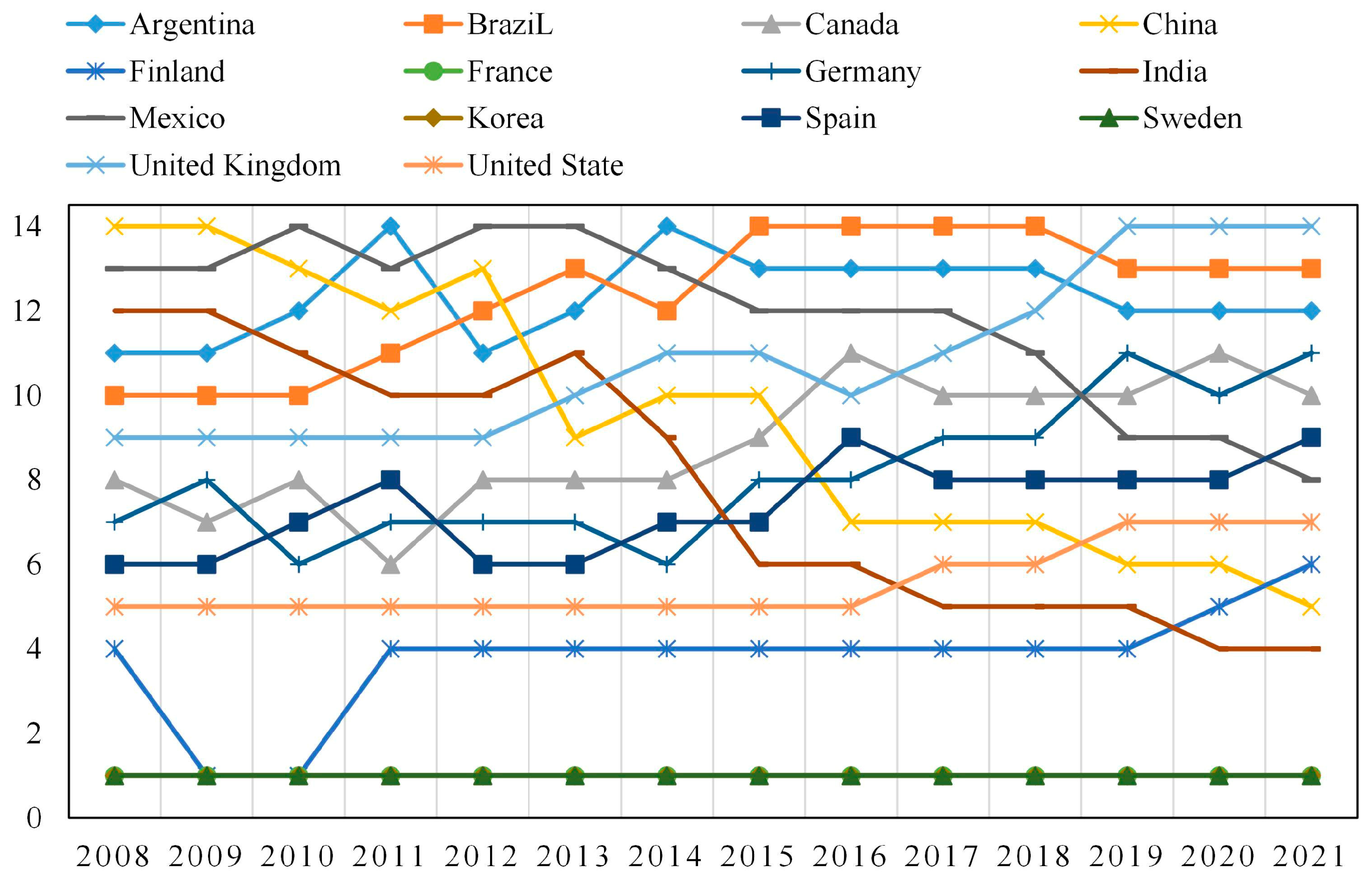
The position of the pathway of the production in 14 countries from past to future is shown in Figure 1.

France, Korea, and Sweden over the period from 2008–2021, and Finland from 2009 to 2010 are explored to obtain a good productivity efficiency of conversation progress from nonrenewable and renewable fuels to electricity and CO₂ emissions through electric generators and turbines. France, Korea, and Sweden are excellent countries, as their scores always maintain a stable and qualified valuation. The empirical results denote that Finland from 2009 to 2010 and these countries are ranked in the first position of electricity generation.

In contrary, the remaining countries and terms of Finland do not attain the productivity efficiency because their estimated scores are less than 1 and always fluctuate in every year. According to the final analysis result, 12 remaining countries, excluding Finland, always have the worst performance. These countries do not approach the top ranking, which only ranges from 5 to 14 from past to future. Especially, the forecasting scores indicate that the efficiency of Argentina, Brazil, Canada, Germany, and the United Kingdom will be dropped consecutively in the future; in addition, their position will remain at the bottom points. China and India demonstrate an upward trend over the whole term, and they can increase sharply in the future; however, their efforts have not reached the productivity efficiency. Mexico, Spain, and United State display fluctuations smoothly in every year.

The empirical results discover some inefficient terms that they must be improved. Section 4.3 suggests a solution based on the principle of an undesirable model. According to the previous researches, the CO₂ emissions from the renewable fuels are less than non-renewable fuels [36]. Thus, the CO₂ emissions can be cut down by augmenting the renewable fuels and by reducing the non-renewable fuels. By the way, the air pollutants from emissions will be reduced, and the environment will be restored.

5. Conclusions

Economic development requires a large demand of electricity energy sources to operate machines in households and factories, so the extension of electricity generation is necessary to meet with the need of users. Augmenting the electrical energy is accompanied by increasing CO₂ emissions. The efficient conversation from primary fuels to electricity generation and CO₂ emissions over the period from 2008 to 2021 is employed by combining the Holt–Winters and undesirable models.

Estimated data in the period of 2018–2021 are calculated by the Holt–Winters model based on the historical data over the period from 2008–2017. The forecasting result describes the usage of nonrenewable and renewable fuels, electricity generation, and CO₂ emissions in the future. The prediction data reveal high accuracy valuations when the average of MAPE indicator is 3.74%.

From the actual and estimated data of variables, including nonrenewable fuel, renewable fuel, electricity generation, and CO₂ emissions in 14 countries all over the world during the period from 2008–2021, the study observes the scores that are calculated by the undesirable model to evaluate the productivity efficiency of the electricity production process in electricity industry. The empirical results manifest the impact level of electricity industry on the environment. In addition, the slacks propose a solution to improve the inefficient terms.

The study determines the productivity efficiency while converting the primary fuels to electricity generation and CO₂ emissions, but limitations remain. First, inputs and outputs are not posted, so the next study needs to have more variables, e.g., employees, equipment, and profit, to assess depth and specification of electricity generation. Second, the undesirable model only gives the maximum efficiency as 1; and, as any countries (DMU) approach the performance, they are at the same top position. Thus, ranking countries will be more specific if the further research applies a super-SBM model into computing the scores. Moreover, estimating the efficiency change of each country will more specific, and future research should use models such as Windows, Malmquist Productivity Index, or bootstrap DEA [37].

References

- Hui, Z.; Danxiang, A. Environment, energy and sustainable economic growth. Proced. Eng. 2011, 21, 513–519. [Google Scholar] [CrossRef]
- Timothy, G.W.; Michael, R.W.W.; Petar, S.V.; Jiři, J.K. Energy ratio analysis and accounting for renewable and non-renewable electricity generation: A review. Renew. Sustain. Energy Rev. 2018, 98, 328–345. [Google Scholar]
- Bob, E.; Godfrey, B.; Stephen, P.; Janet, R. Energy Systems and Sustainability; Oxford University: New York, NY, USA, 2003. [Google Scholar]
- Murillo, V.B.; Cassiano, M.P.; Sntonio, C.D.F. Carbon Footprint of Electricity Generation in Brazil: An Analysis of the 2016–2026 Period. Energies 2018, 11, 1412. [Google Scholar] [CrossRef]
- Jiang, L.; Gang, H.; Alexandria, Y. Economic rebalancing and electricity demand in China. Electr. J. 2016, 29, 48–54. [Google Scholar] [CrossRef] [Green Version]
- Chen, T.L. Air Pollution Caused by Coal-fired Power Plant in Middle Taiwan. Int. J. Energy Power Eng. 2017, 6, 121–124. [Google Scholar] [CrossRef]
- Time Series and Forecasting Methods in NCSS. Available online: https://www.ncss.com (accessed on 29 September 2018).
- Seyed Esmaeili, F.; Rostamy-Malkhalifed, M. Data Envelopment Analysis with Fixed Inputs, Undesirable Outputs and Negative Data. J. Data Envel. Anal. Decis. Sci. 2017, 1, 1–6. [Google Scholar] [CrossRef]
- Lawrence, M.S.; Joe, Z. Modeling Undesirable Factors in Efficiency Evaluation. Eur. J. Oper. Res. 2002, 142, 16–20. [Google Scholar] [CrossRef]
- Ekundayo, G. Review of Sustainable Energy and Electricity Generation from Non—Rewneable Energy Sources. J. Energy Technol. Policy 2015, 5, 53–57. [Google Scholar]
- Thomas, A.A.; Leila, H.; Pranav, B.M.; Ikenna, J.O. Comparison of CO2 Capture Approaches for Fossil-Based Power Generation: Review and Meta-Study. Processes 2017, 5, 44. [Google Scholar] [CrossRef]
- Benjamin, D.N.; Su, L.; Jinfeng, L. Improving Flexibility and Energy Efficiency of Post-Combustion CO2 Capture Plants Using Economic Model Predictive Control. Processes 2018, 6, 135. [Google Scholar] [CrossRef]
- Raghuvanshi, S.P.; Chandra, A.; Raghav, A.K. Carbon dioxide emissions from coal based power generation in India. Energy Convers. Manag. 2006, 47, 427–441. [Google Scholar] [CrossRef]
- Lamiaa, A.; Tarek, E.S. Reducing Carbon Dioxide Emissions from Electricity Sector Using Smart Electric Grid Applications. J. Eng. 2013, 2013, 845051. [Google Scholar] [CrossRef]
- Ostertagová, E.; Qstertag, O. The Simple Exponential Smoothing Model. In Proceedings of the Modelling of Mechanical and Mechatronic Systems 2011, Herlany, Slovak Republic, 20–22 September 2011. [Google Scholar]
- Taylor, J.W. Exponential Smoothing with a Damped Multiplicative Trend. Int. J. Forecast. 2003, 19, 715–725. [Google Scholar] [CrossRef]
- Taylor, J.W. Short-Term Electricity Demand Forecasting Using Double Seasonal Exponential Smoothing. J. Oper. Res. Soc. 2003, 54, 799–805. [Google Scholar] [CrossRef]
- Berm’udez, J.D.; Segura, J.V.; Vercher, E. Bayesian forecasting with the Holt–Winters model. J. Oper. Res. Soc. 2010, 61, 164–171. [Google Scholar] [CrossRef]
- Puah, Y.J.; Huang, Y.F.; Chua, K.C.; Lee, T.S. River catchment rainfall series analysis using additive Holt–Winters method. J. Earth Syst. Sci. 2016, 125, 269–283. [Google Scholar] [CrossRef]
- Rahman, M.H.; Salma, U.; Hossain, M.M.; Khan, M.T.F. Revenue Forecasting using Holt–Winters Exponential Smoothing. Res. Rev. J. Stat. 2017, 5, 19–25. [Google Scholar]
- Ashraf, A.S. Using Multiple Seasonal Holt-Winters Exponential Smoothing to Predict Cloud Resource Provisioning. Int. J. Adv. Comput. Sci. Appl. 2016, 7, 91–96. [Google Scholar] [CrossRef]
- Medy, W.P.; Ema, U. Analysis of Moving Average and Holt-Winters Optimaization by Using Golden Section for Ritase Forecasting. J. Theor. Appl. Inf. Technol. 2017, 95, 6575–6584. [Google Scholar]
- Tone, K. A slacks-based measure of efficiency in data envelopment analysis. Eur. J. Oper. Res. 2001, 130, 498–509. [Google Scholar] [CrossRef] [Green Version]
- Tone, K. A slack-based measure of super-efficiency in data envelopment analysis. Eur. J. Oper. Res. 2002, 143, 34–41. [Google Scholar] [CrossRef]
- Tone, K. Dealing with Undesirable Outputs in DEA: A Slacks-Based Measure (SBM) Approach; National Graduate Institute for Policy Studies: Tokyo, Japan, 2003. [Google Scholar]
- Kuo, H.F.; Chen, H.L.; Tsou, K.W. Analysis of Farming Environmental Efficiency Using a DEA Model with Undesirable Outputs. APCBEE Procedia 2014, 10, 154–158. [Google Scholar] [CrossRef]
- Goto, M.; Takahashi, T. Operational and Environmental Efficiencies of Japanese Electric Power Companies from 2003 to 2015: Influence of Market Reform and Fukushima Nuclear Power Accident. Math. Probl. Eng. 2017, 2017, 4936595. [Google Scholar] [CrossRef]
- Ozkan, N.F.; Ulutas, B.H. Efficiency analysis of cement manufacturing facilities in Turkey considering undesirable outputs. J. Clean. Prod. 2017, 156, 932–938. [Google Scholar] [CrossRef]
- BP Statistical Review of World Energy. Available online: https://www.bp.com (accessed on 30 September 2018).
- Nonrenewable Sources. Available online: https://www.eia.gov (accessed on 28 September 2018).
- Renewable Sources. Available online: https://www.eia.gov (accessed on 28 September 2018).
- Beverton, R.J.H.; Sidney, J.H. On the Dynamics of Exploited Fish Populations; Great Britain Fishery Investment: London, UK, 1957. [Google Scholar]
- Winter, P.R. Forecasting Sale by Exponentially Weighted Moving Averages. Manag. Sci. 1960, 6, 324–342. [Google Scholar] [CrossRef]
- Lewis, C.D. Industrial and Business Forecasting Methods: A Practical Guide to Exponential Smoothing and Curve Fitting; Butterworth Scientific: London, UK, 1982. [Google Scholar]
- López, F.J.; Ho, J.C.; Ruiz-Torres, A.J. A computational analysis of the impact of correlation and data translation on DEA efficiency score. J. Ind. Prod. Eng. 2016, 33, 192–204. [Google Scholar] [CrossRef]
- Robert, J.P. Cutting carbon emissions from electricity generation. Electr. J. 2017, 30, 41–61. [Google Scholar] [CrossRef]
- Badunenko, O.; Tauchmann, H. Simar and Wilson Two-Stage Efficiency Analysis for Stata; FriedrichAlexander-Universität Erlangen-Nürnberg, Institute for Economics: Erlangen, German, 2018. [Google Scholar]
Figure 1.
Ranking the pathway of production.