A High-Order Numerical Manifold Method for Darcy Flow in Heterogeneous Porous Media

Abstract

One major challenge in modeling Darcy flow in heterogeneous porous media is simulating the material interfaces accurately. To overcome this defect, the refraction law is fully introduced into the numerical manifold method (NMM) as an a posteriori condition. To achieve a better accuracy of the Darcy velocity and continuous nodal velocity, a high-order weight function with a continuous nodal gradient is adopted. NMM is an advanced method with two independent cover systems, which can easily solve both continuous and discontinuous problems in a unified form. Moreover, a regular mathematical mesh, independent of the physical domain, is used in the NMM model. Compared to the conforming mesh of other numerical methods, it is more efficient and flexible. A number of numerical examples were simulated by the new NMM model, comparing the results with the original NMM model and the analytical solutions. Thereby, it is proven that the proposed method is accurate, efficient, and robust for modeling Darcy flow in heterogeneous porous media, while the refraction law is satisfied rigorously.

1. Introduction

Heterogeneity is the natural property of the geologic structure in groundwater systems. A real groundwater system can be regarded as a combination of several homogeneous subdomains. However, the contrast between the hydraulic conductivities of two adjacent subdomains presents a great challenge for numerical modeling. The two major limitations of modeling Darcy flow in heterogeneous porous media by conventional numerical methods are as follows. (1) The precision of the Darcy velocity (also known as specific discharge) is deficient, as the existing method usually solves the hydraulic head first, then computes the Darcy velocity by taking the derivation of the hydraulic head field. (2) The refraction law, which is expressed as the continuity of normal flux and discontinuity of tangential flux on the interface [1], can be hardly achieved. For the first limitation, the precision of the Darcy velocity decreases to a low order after derivation, and that leads to the discontinuity of the Darcy velocity around a node. For the second limitation, Cainelli et al. [2] summarized the accuracy of classic numerical schemes, such as the finite element method (FEM) [3,4] and finite volume method (FVM) [5,6,7], for modeling flow in heterogeneous formations. Results show that the above methods cannot satisfy the refraction law rigorously when the contrast of conductivities is large, hence the local computation error can be non-negligible.

In order to improve the first limitation (i.e., the lack of precision of the velocity solution), there are two different approaches. The first way is using some post-processing techniques to improve the velocity solution after the hydraulic head is solved [8,9,10]. These methods are efficient, as they can be easily modified from the original FEM approach. For example, in Yeh’s model [9], the head solution is substituted into the variational formula of Darcy’s law, which is then directly solved by the same FEM approach. Although normal flux across the interface is continuous, the tangential component still cannot satisfy refraction law when facing contrasting hydraulic conductivities. The other way is to solve the head and velocity simultaneously, which is known as the mixed finite element method (MFEM) [11,12]. However, iterations are still required for MFEM, making the calculation time-consuming [13].

Imposing the refraction law to the governing equation as an additional constraint condition is an efficient approach to dealing with the second limitation. For example, Zhou et al. [14] proposed a modified Yeh’s method using a post-processing scheme to enforce the refraction law across material interfaces. Thus, iterations are required for the scheme to achieve convergence. Additionally, Xie et al. [15] developed a domain decomposed finite element method for solving the Darcy velocity in heterogeneous porous media without iterations. The basic idea is to separate the problem domain into several subdomains by material interfaces with coercive refraction law. Nevertheless, the above FEM-based methods are still mesh-dependent, which is inconvenient for pre-processing, especially when material interfaces are complex.

The numerical manifold method (NMM) first presented by Shi [16,17] can be regarded as a generalization to the conventional FEM. Due to the feature of solving both continuous and discontinuous problems in a unity frame, NMM is widely used in mechanical analysis, such as crack propagation [18,19,20,21], rock slopes failure [22,23,24], and dynamic problems [25,26,27,28]. NMM also played an important role in fluid flow modeling. Ohnishi et al. [29] presented a node shift method based on NMM for 2D saturated–unsaturated unsteady seepage simulation. Zhang et al. [30] solved Navier–Stokes equations directly by NMM, modeling unsteady incompressible viscous flow. Furthermore, NMM models for unconfined seepage flow in homogeneous media were reported [31,32]. However, it cannot exploit the properties of NMM to deal with homogeneous problems, compared with other continuous methods like FEM. Aiming to simulate Darcy flow in heterogeneous media, Hu et al. [33,34,35] developed a continuous approach with jump functions and a discontinuous approach with Lagrange multipliers, by enforcing the continuity of normal flux across material interfaces, while the refraction law for tangential flux is ignored. Zheng et al. [36] also proposed an NMM model for unconfined seepage flow by adopting the moving least squares (MLS) interpolation. Hence, NMM is an efficient approach for heterogeneous seepage problems. However, improving the accuracy of modeling, that is still a great challenge.

In this work, we developed a high-order NMM model for Darcy flow in heterogeneous porous media with a nodal-continuous weight function, as well as a local cover function derived by first order approximation of Taylor expansion. Then we introduced refraction law into the NMM model as an a posteriori constraint condition entirely to ensure that material interfaces are simulated correctly. The proposed NMM model has the following advantages. (1) The accuracy of the Darcy velocity solution is high and keeps continuous around a node, both of which are significant for modeling underground flow as well as solute transport. (2) The treatment of material interfaces in the NMM model is accurate and efficient, especially when facing various materials with interfaces intersecting each other, by taking full advantage of NMM’s dual cover systems. More details of the proposed NMM model will be discussed in the following sections.

The framework of this paper is organized as follows. Section 2 briefly introduces some basic concepts of the original NMM theory. Then, the new NMM formation for Darcy flow in heterogeneous porous media is derived in Section 3. With the aim of testing the reliability of the proposed NMM model, numerical examples are simulated in Section 4. Finally, main conclusions and discussions are given in Section 5.

2. Basic Theory of NMM

Basic concepts of NMM are introduced in this section, including the dual cover systems and the manifold elements. The local approximation on physical covers and the global approximation on manifold elements are proposed next. This section shows that the NMM is suitable for modeling discontinuous problems because of the efficient meshing algorithm and the treatment of discontinuous boundaries.

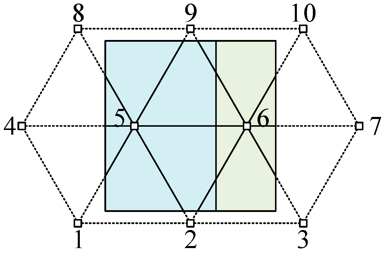
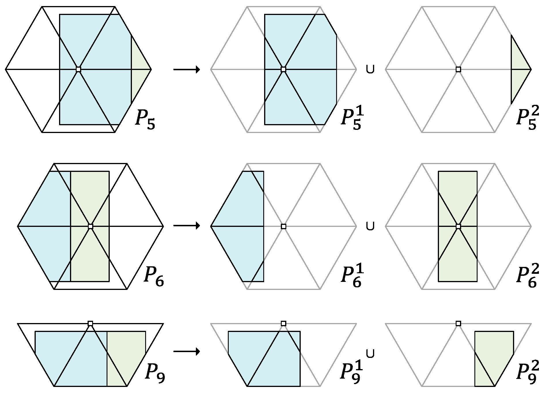
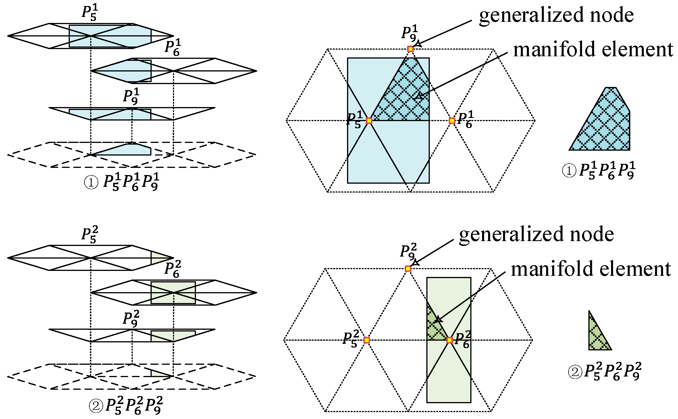
2.1. Dual Cover Systems and Manifold Elements

The basic concepts of NMM include mathematical cover (MC), physical cover (PC), and manifold element (ME). The mathematical cover system is a set of patches which completely cover the whole physical domain. Thus, each patch is an MC. PCs are generated from MCs, cutting via boundaries or cracks and material interfaces inside the physical area. More remarkably, the shape of MC may be arbitrary, which is not necessary in coinciding with the boundaries as long as the whole domain is covered. Here, standard FEM mesh is used to generate MCs for convenience, and the density of mesh decides computational accuracy.

A simple example is given to illustrate the above concepts. As shown in Figure 1, a rectangular domain is divided into two different materials by a vertical interface. A regular triangular mesh is used to form MCs in this example. Each node in the mesh is defined as a star, and MCs are formed by triangles adjacent to a star, denoted as $P_i$, where the subscribe $i$ is the number of the star. Thus, the standard shape of MC in this example is a hexagon (i.e., $P_5$ and $P_6$) combined by six triangles. However, quadrangular or triangular MCs may be made using fewer triangles on the boundaries (i.e., $P_9$).

MCs are divided into independent parts by outside boundaries or material interfaces. Each part of MCs is regarded as a PC. This is denoted as $P_i^j$, where the superscript $j$ is the number of the PC belonging to the i-th MC. As illustrated in Figure 2, $P_5$ is divided into $P_5^1$ and $P_5^2$ by boundaries and material interface. Similarly, $P_6$ is divided into $P_6^1$ and $P_6^2$, and $P_9$ is divided into $P_9^1$ and $P_9^2$.

After generating the cover systems, manifold elements—the basic integral region of the weak form of the problems—are defined as the overlapping areas of PCs. As exhibited in Figure 3, MEs are regarded as the common area of three layers of PCs when adopting triangular finite element mesh. Therefore, the star of the corresponding PCs is considered as a generalized node of the ME in NMM. This is different to the concept of nodes in FEM. For simplicity, the generalized node will be termed as “node” for the rest of this paper. In addition, the shape of MEs are generally triangular, except for the MEs adjacent to boundaries or interfaces, which may have an arbitrary shape. As long as the MCs are based on triangular mesh, the number of generalized nodes of an ME is three. As shown in Figure 3, ME$①$ is overlapped by $P_5^1$, $P_6^1$, and $P_9^1$. Thus, ME$①$ is termed as $P_5^1{P}_6^1{P}_9^1$, and ME$②$ is similarly termed as $P_5^2{P}_6^2{P}_9^2$. In this way, the discontinuity of the triangular element cut by boundaries or material interface is presented by NMM.

Theoretically, NMM is a kind of partition of unity method (PUM). Its important feature is that the global approximation is established by combining local approximations using a PU function. According to the theory of NMM, local approximation is defined on each PC as a cover function, while global approximation on each ME is built through combining cover functions using weight functions, which are the same as PU functions. Details of NMM approximation is introduced in the following two subsections.

2.2. Local Approximation on Physical Covers

Local approximation is defined on each PC, representing the local field variables. That is, normally expressed as

$${\phi }_i\left(x\right)=p^T\left(x\right)·\mathit{a},i\in \left[1,n^{PC}\right]$$

(1)

where $n^{PC}$ is the total number of PCs, x are coordinates of points within the i-th PC, $\mathit{a}$ is a vector of unknown coefficients, and $p^T\left(x\right)$ is the vector of polynomials bases. The latter can be expressed as

$$\begin{gathered} p^T\left(x\right)=\left[1,x,y\right] \\ {p}^T\left(x\right)=\left[1,x,y,x^2,xy,y^2\right] \\ {p}^T\left(x\right)=\left[1,x,y,x^2,xy,y^2,\cdots ,x^n,\cdots ,y^n\right] \end{gathered}$$

(2)

for the first, second, and $n$-th order approximation, respectively, where $n$ is a positive integer representing the approximation order.

However, in contrast with polynomial bases, specific bases can be selected as $p^T\left(x\right)$ on each PC for achieving batter approximation. As a result, NMM has the ability to combine analytical solution with numerical method, that is to say, corresponding analytical solution can be chosen as the local approximation in the key position of problem domain, while polynomials bases are adopted on the rest of domain. Thus, a more accurate and efficient solution can be achieved. For example, Williams’ displacement series are usually used as the local approximation near a crack tip for crack problems, making the stress solution around tip more accurate and reliable [18,19].

2.3. Global Approximation on Manifold Elements

Based on the NMM theory, global approximation is defined on each ME. The field variables $\phi$ on MEs are obtained by taking a weighted average of local approximations on corresponding PCs. Therefore, global approximation can be expressed as

$$\phi \left(x,y\right)={\displaystyle \sum }_{i=1}^{N_{PC}}{w}_i\left(x,y\right){\phi }_i\left(x,y\right)$$

(3)

where $N_{PC}$ is the number of PCs on the ME and $w_i\left(x,y\right)$ is weight function of the i-th PC, which satisfies

$$\{\begin{array}{c}{w}_i\left(x,y\right)>0\left(x,y\right)\in U_i\\ w_i\left(x,y\right)=0\left(x,y\right)\notin U_i\end{array}$$

(4)

where $U_i$ is the geometric range of the i-th PC.

3. Steady Darcy Flow in Heterogeneous Porous Media by NMM

In this section, NMM formulation of steady Darcy flow in heterogeneous porous media is derived, including treatments for boundaries and material interfaces.

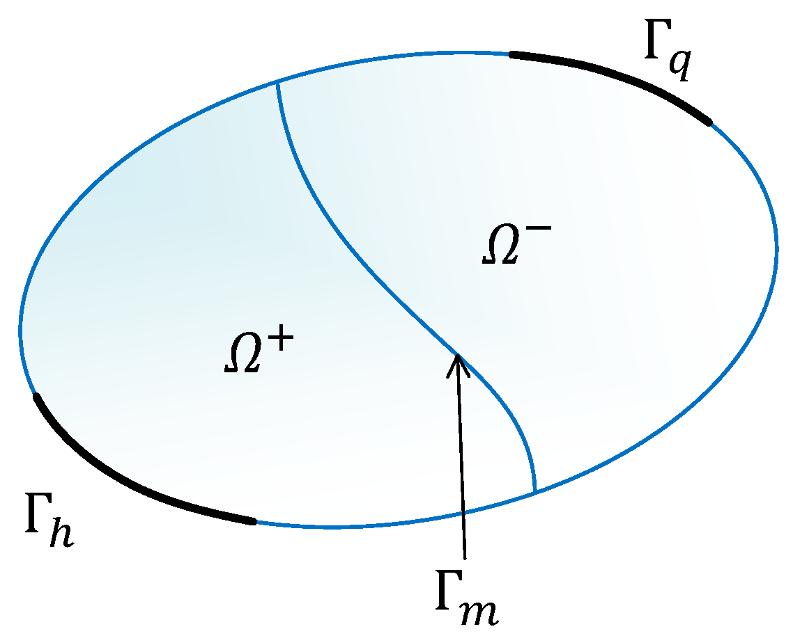
3.1. Governing Equations

Considering 2D steady Darcy flow in heterogeneous porous media, the continuity equation is derived using the conservation of mass, expressed as

$${\nabla }^T\mathit{v}+Q=0$$

(5)

where $\nabla$ is the gradient operator, $\mathit{v}$ is the Darcy velocity or specific discharge, and $Q$ is the source term. The constitutive equation for Darcy flow is Darcy’s law, which means there is a linear relationship between the Darcy velocity and the hydraulic gradient. This is given as

$$\mathit{v}=-\mathit{K}\nabla h$$

(6)

where $\mathit{K}$ is the permeability tensor and $h$ is the hydraulic head. Substituting Equation (6) into Equation (5), the governing differential equation can be rewritten as

$$-{\nabla }^T\left(\mathit{K}\nabla h\right)+Q=0.$$

(7)

As shown in Figure 4, the associated boundary conditions can be written as

$$h=\overline{h}$$

(8)

for the Dirichlet condition on ${\mathsf{\Gamma }}_h$,

$$q_n=\overline{q}$$

(9)

for the Neumann condition on ${\mathsf{\Gamma }}_q$, and

$$\begin{gathered} h^{+}=h^{-} \\ {v}_n^{+}=v_n^{-} \\ {v}_s^{+}·k^{-}=v_s^{-}·k^{+} \end{gathered}$$

(10)

for the refraction law across the material interface ${\mathsf{\Gamma }}_m$, where $\overline{h}$ is the given hydraulic head on ${\mathsf{\Gamma }}_h$, $q_n$ is normal flux on ${\mathsf{\Gamma }}_q$, $\overline{q}$ is the given flux, and $v_n$ and $v_s$ are normal and tangential components of the Darcy velocity, respectively. Superscript $+$ and $–$ represent the two sides of the material interface ${\mathsf{\Gamma }}_m$. In addition, $v_n$ and $v_s$ can be expressed as

$$v_n=\mathit{v}·\mathit{n}$$

(11a)

$$v_s=\mathit{v}·\mathit{s}$$

(11b)

where $\mathit{n}$ and $\mathit{s}$ are the normal unit vector and tangential unit vector, respectively.

The first two conditions of refraction law can be easy deduced. They represent the continuity of the hydraulic head and normal flux. Here we briefly prove the third condition for tangential flux. As shown in Figure 5, a rectangular domain is divided into two different materials ${\mathsf{\Omega }}_1$ and ${\mathsf{\Omega }}_2$, both of which are homogeneous and isotropic media. The permeability coefficients are $k^{+}$ and $k^{-}$. Suppose fluid flows upside to downside, and ${\theta }_1$ and ${\theta }_2$ are the angles between the direction of the Darcy velocity and the normal direction of the material interface in ${\mathsf{\Omega }}_1$ and ${\mathsf{\Omega }}_2$, respectively. From Equation (10) it follows that

$$j_s^{+}=j_s^{-}$$

(12)

across the material interface, where $j$ is hydraulic gradient. Thus, the tangential component of the hydraulic gradient is continuous across the material interface. According to Darcy’s law, the tangential component of the Darcy velocity can be expressed as

$$\begin{gathered} v_s^{+}=k^{+}·j_s^{+} \\ {v}_s^{-}=k^{-}·j_s^{-} \end{gathered}$$

(13)

Substituting Equation (13) into Equation (12) and considering the geometric condition, the tangential velocity in two sides of the interface satisfies

$$\frac{v_s^{+}}{v_s^{-}}=\frac{k^{+}}{k^{-}}=\frac{\tan {\theta }_1}{\tan {\theta }_2}$$

(14)

which is equivalent to the third condition in Equation (10).

Through this subsection, NMM formation for Darcy flow in heterogeneous media is derived. The main purpose of this study is to solve the differential equation of Darcy flow, Equation (7) with constraint conditions of Equations (8)–(10) for the hydraulic head and the Darcy velocity using NMM.

3.2. NMM Interpolations

In this paper, Taylor series expansion was applied to establish the local approximation on each PC. Thus, the base function on a PC can be adopted by first order approximation of the Taylor expansion of the corresponding node. According to Equation (1), the local approximation of the hydraulic head on each PC, $h_i\left(x\right)$, can be written as

$$h_i\left(x\right)=p^T\left(x\right)·\mathit{a},i\in \left[1,n^{PC}\right]$$

(15)

where $\mathit{a}$ is a vector of unknown coefficients, and bases are expressed as

$$p^T\left(x\right)=\left[1,x-x_i,y-y_i\right]$$

(16)

where $x_i$ and $y_i$ are coordinates of node i.

Substituting Equation (16) into Equation (15), the local approximation on PCs can be rewritten as

$$h_i\left(x\right)=h_i\left(x_i,y_i\right)+\left(x-x_i\right)\frac{\partial h_i\left(x_i,y_i\right)}{\partial x}+\left(y-y_i\right)\frac{\partial h_i\left(x_i,y_i\right)}{\partial y}.$$

(17)

Comparing with conventional polynomials bases, the exact physical meanings of the unknown coefficients, the corresponding hydraulic head, and the gradient on each node are achieved.

Then, global approximation on each ME can be derived as

$$h\left(x\right)={\displaystyle \sum }_{i=1}^3{w}_i\left(x\right)h_i\left(x\right)=\mathit{N}\mathit{a}$$

(18)

where $\mathit{N}$ is the shape function, expressed as

$$\mathit{N}={\displaystyle \sum }_{i=1}^3{w}_i\left(x\right)p^T\left(x\right)$$

(19)

and $w_i\left(x\right)$ is the weight function on the i-th PC, originally used in mechanics problems [37,38]. This is expressed as

$$w_i\left(x\right)=L_i+L_i^2\left(L_j+L_m\right)-L_i\left(L_j^2+L_m^2\right)$$

(20)

where $L_i$ ($i=1,2,3$) are area coordinates of the triangular finite element. The above weight function has four important features:

(1)

the Kronecker delta property ($w_i\left(x_j\right)={\delta }_{ij}$ ($i,j=1,2,3$)),

(2)

the non-negative property ($0\le w_i\left(x\right)\le 1$ ($x\in U_i$)),

(3)

the partition of the unity condition (${{\displaystyle \sum }}_{i=1}^3{w}_i\left(x\right)=1$),

(4)

and a nodal gradient of zero of the weight function.

Therefore, the gradient of the hydraulic head solution at a generalized node is continuous, because of the last property, which is of great importance in this study. A continuous Darcy velocity can be then derived by Darcy’s law at nodes. However, the discontinuity of velocity still exists on element edges.

3.3. Discrete Equations

The weak form of governing Equation (7) is derived by the weighted residual method, and then the functional expression derived by the variational principle can be written as [39]

$$\mathsf{\Pi }\left(h\right)={{\displaystyle \int }}_{\mathsf{\Omega }}^{}\left[\frac{1}{2}{\left(\nabla h\right)}^T\left(\mathit{K}\nabla h\right)-hQ\right]d\mathsf{\Omega }-{{\displaystyle \int }}_{{\mathsf{\Gamma }}_q}^{}h\overline{q}d\mathsf{\Gamma }.$$

(21)

In each ME, the hydraulic head, $h$, is defined as

$$h=\mathit{N}\mathit{a}$$

(22)

where $\mathit{N}$ is the shape function, and $\mathit{a}$ is the unknowns.

The hydraulic gradient, $\mathit{j}$, is defined as

$$\mathit{j}=\nabla h=\nabla \mathit{N}\mathit{a}=\mathit{B}\mathit{a}$$

(23)

where $\mathit{B}=\nabla \mathit{N}$.

The Darcy velocity, $\mathit{v}$, is expressed as

$$\mathit{v}=-\mathit{K}\mathit{j}=-\mathit{K}\mathit{B}\mathit{a}$$

(24)

where $\mathit{K}$ is the permeability tensor.

By substituting Equations (22)–(24) into Equation (21), the functional expression of each ME can be obtained.

$${\mathsf{\Pi }}^e={{\displaystyle \int }}_{{\mathsf{\Omega }}^e}^{}\frac{1}{2}{\mathit{a}}^T{\mathit{B}}^T\mathit{K}\mathit{B}\mathit{a}d\mathsf{\Omega }-{{\displaystyle \int }}_{{\mathsf{\Omega }}^e}^{}{\mathit{a}}^T{\mathit{N}}^{T}Qd\mathsf{\Omega }-{{\displaystyle \int }}_{{\mathsf{\Gamma }}_q}^{}{\mathit{a}}^T{\mathit{N}}^T\overline{q}d\mathsf{\Gamma }$$

(25)

where ${\mathsf{\Omega }}^e$ is the domain of each ME. Therefore, the functional expression of the whole problem domain, Equation (21), can be rewritten in a matrix form

$$\mathsf{\Pi }=\frac{1}{2}\left(\begin{array}{ccc}{a}_1& \cdots & a_n\end{array}\right)\left(\begin{array}{ccc}{C}_{11}& \dots & C_{1n}\\ ⋮& \ddots & ⋮\\ C_{n1}& \dots & C_{nn}\end{array}\right)\left(\begin{array}{c}{a}_1\\ ⋮\\ a_n\end{array}\right)-\left(\begin{array}{ccc}{a}_1& \cdots & a_n\end{array}\right)\left(\begin{array}{c}{F}_1\\ ⋮\\ F_n\end{array}\right)=\frac{1}{2}{\mathit{a}}^T\mathit{C}\mathit{a}-{\mathit{a}}^T\mathit{F}$$

(26)

where $n$ is the number of unknowns in the problem, $\mathit{C}$ is the conductivity matrix with $n\times n$ components, and $\mathit{F}$ is the flux term with $n$ components, expressed as

$$\mathit{C}={{\displaystyle \int }}_{\mathsf{\Omega }}^{}{\mathit{B}}^T\mathit{K}\mathit{B}d\mathsf{\Omega }$$

(27)

$$\mathit{F}={{\displaystyle \int }}_{\mathsf{\Omega }}^{}{\mathit{N}}^{T}Qd\mathsf{\Omega }+{{\displaystyle \int }}_{{\mathsf{\Gamma }}_q}^{}{\mathit{N}}^T\overline{q}d\mathsf{\Gamma }$$

(28)

respectively. Their components can be derived by taking the derivatives with the unknowns, expressed as

$$C_{ij}=\frac{{\partial }^2\mathsf{\Pi }}{\partial a_i\partial a_j}$$

(29)

$$F_i=-\frac{\partial \mathsf{\Pi }}{\partial a_i}.$$

(30)

According to the variational principle, the solution of the weak form of the differential equation is equivalent to a function $\mathit{a}$ which makes $\mathsf{\Pi }$ stationary with respect to arbitrary changes of $\mathsf{\delta }\mathit{a}$, that is

$$\mathsf{\delta }\mathsf{\Pi }=\frac{\partial \mathsf{\Pi }}{\partial a_1}\delta a_1+\frac{\partial \mathsf{\Pi }}{\partial a_2}\delta a_2+\dots +\frac{\partial \mathsf{\Pi }}{\partial a_n}\delta a_n=0$$

(31)

where $\delta a_1$, $\delta a_2$, …, $\delta a_n$ are arbitrary changes. Therefore, Equation (7) reduces to a standard linear form as

$$\frac{\partial \mathsf{\Pi }}{\partial a}=\left\{\begin{array}{c}\frac{\partial \mathsf{\Pi }}{\partial a_1}\\ ⋮\\ \frac{\partial \mathsf{\Pi }}{\partial a_n}\end{array}\right\}=0$$

(32)

which can be rewritten as a matrix form

$$\mathit{C}\mathit{a}=\mathit{F}$$

(33)

and

$$\left(\begin{array}{ccc}{C}_{11}& \dots & C_{1n}\\ ⋮& \ddots & ⋮\\ C_{n1}& \dots & C_{nn}\end{array}\right)\left\{\begin{array}{c}{a}_1\\ ⋮\\ a_n\end{array}\right\}=\left\{\begin{array}{c}{F}_1\\ ⋮\\ F_n\end{array}\right\}.$$

(34)

Therefore, the governing differential equation, Equation (7) is transformed a system of linear equations (Equation (34)), which can be easily solved. In addition, the hydraulic head and Darcy velocity can be obtained using Equations (22) and (24), respectively.

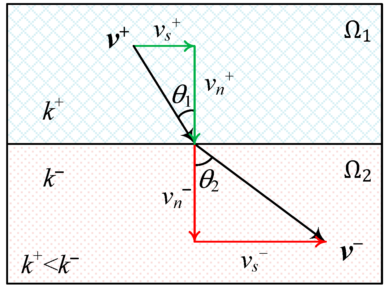
3.4. Treatments for Boundaries and Material Interfaces

In Section 3.3, the Dirichlet boundary condition and refraction law across material interfaces are not involved. The treatments for boundaries and material interfaces are introduced in this subsection. Generally, two basic methods to impose additional constraints are the Lagrange multiplier method and the penalty method. Although the Lagrange multiplier method can achieve an accurate solution, additional degrees of freedom must be introduced into the governing function, which usually leads to computational difficulties. The penalty method is more convenient as it does not require a change of the size of the coefficient matrix and is free of the above drawbacks of the Lagrange multiplier method. Note that the penalty number should be neither too small nor too large to enforce the constraints and avoid computational difficulties. In this study, the penalty method is adopted, and penalty number $\mathsf{\alpha }$ is determined as ${10}^6$. The accuracy and robustness are verified by a series of numerical tests.

In addition, the treatments of material interfaces by existing methods are inadequate. In this paper, additional constraints of the Dirichlet boundary condition and refraction law across the material interface are introduced by forming a new functional

$${\mathsf{\Pi }}^{\ast }=\mathsf{\Pi }+{\mathsf{\Pi }}_D+{\mathsf{\Pi }}_m$$

(35)

in which ${\mathsf{\Pi }}_D$ is the Dirichlet boundary condition term and ${\mathsf{\Pi }}_m$ is material interface term.

For the Dirichlet boundary condition, ${\mathsf{\Pi }}_D$ is expressed as

$${\mathsf{\Pi }}_D=\frac{\alpha }{2}{{\displaystyle \int }}_{{\mathsf{\Gamma }}_D}^{}{\left(h-\overline{h}\right)}^{2}d\mathsf{\Gamma }$$

(36)

where $\alpha$ is the penalty number. Thus, the components of the conductivity matrix, $C_{ij}$, and the flux term, $F_i$, for the equilibrium equation can be derived as

$$C_{ij}=\frac{{\partial }^2{\mathsf{\Pi }}_D}{\partial a_i\partial a_j}=\mathsf{\alpha }{{\displaystyle \int }}_{{\mathsf{\Gamma }}_D}^{}{\mathit{N}}^T\mathit{N}d\mathsf{\Gamma }$$

(37)

$$F_i=-\frac{\partial \mathsf{\Pi }}{\partial a_i}=\alpha {{\displaystyle \int }}_{{\mathsf{\Gamma }}_D}^{}{\mathit{N}}^T\overline{h}d\mathsf{\Gamma }.$$

(38)

For the material interface, ${\mathsf{\Pi }}_m$ can be written into three parts

$${\mathsf{\Pi }}_m={\mathsf{\Pi }}_m^a+{\mathsf{\Pi }}_m^b+{\mathsf{\Pi }}_m^c.$$

(39)

Each part of ${\mathsf{\Pi }}_m$ can be expressed as

$${\mathsf{\Pi }}_m^a=\frac{\alpha }{2}{{\displaystyle \int }}_{{\mathsf{\Gamma }}_m}^{}{\left(h^{+}-h^{-}\right)}^{2}d\mathsf{\Gamma }$$

(40a)

$${\mathsf{\Pi }}_m^b=\frac{\alpha }{2}{{\displaystyle \int }}_{{\mathsf{\Gamma }}_m}^{}{\left({\mathit{v}}_{\mathit{n}}^{+}-{\mathit{v}}_{\mathit{n}}^{-}\right)}^{2}d\mathsf{\Gamma }$$

(40b)

$${\mathsf{\Pi }}_m^c=\frac{\alpha }{2}{{\displaystyle \int }}_{{\mathsf{\Gamma }}_m}^{}{\left(\frac{{\mathit{v}}_{\mathit{s}}^{+}}{{\mathit{k}}^{+}}-\frac{{\mathit{v}}_{\mathit{s}}^{-}}{{\mathit{k}}^{-}}\right)}^{2}d\mathsf{\Gamma }.$$

(40c)

Thus, the components of the conductivity matrix can be respectively derived as

$$C_{ij}=\frac{{\partial }^2{\mathsf{\Pi }}_m^a}{\partial a_i\partial a_j}=\mathsf{\alpha }{{\displaystyle \int }}_{{\mathsf{\Gamma }}_m}^{}\left(\begin{array}{cc}{\left({\mathit{N}}^{+}\right)}^T{\mathit{N}}^{+}& -{\left({\mathit{N}}^{+}\right)}^T{\mathit{N}}^{-}\\ -{\left({\mathit{N}}^{-}\right)}^T{\mathit{N}}^{+}& {\left({\mathit{N}}^{-}\right)}^T{\mathit{N}}^{-}\end{array}\right)d\mathsf{\Gamma }$$

(41a)

$$C_{ij}=\frac{{\partial }^2{\mathsf{\Pi }}_m^b}{\partial a_i\partial a_j}=\mathsf{\alpha }{{\displaystyle \int }}_{{\mathsf{\Gamma }}_m}^{}\left(\begin{array}{cc}{\left({\mathit{K}}^{+}{\mathit{B}}^{+}\mathit{n}\right)}^T\left({\mathit{K}}^{+}{\mathit{B}}^{+}\mathit{n}\right)& -{\left({\mathit{K}}^{+}{\mathit{B}}^{+}\mathit{n}\right)}^T\left({\mathit{K}}^{-}{\mathit{B}}^{-}\mathit{n}\right)\\ -{\left({\mathit{K}}^{-}{\mathit{B}}^{-}\mathit{n}\right)}^T\left({\mathit{K}}^{+}{\mathit{B}}^{+}\mathit{n}\right)& {\left({\mathit{K}}^{-}{\mathit{B}}^{-}\mathit{n}\right)}^T\left({\mathit{K}}^{-}{\mathit{B}}^{-}\mathit{n}\right)\end{array}\right)d\mathsf{\Gamma }$$

(41b)

$$C_{ij}=\frac{{\partial }^2{\mathsf{\Pi }}_m^c}{\partial a_i\partial a_j}=\mathsf{\alpha }{{\displaystyle \int }}_{{\mathsf{\Gamma }}_m}^{}\left(\begin{array}{cc}{\left({\mathit{B}}^{+}\mathit{s}\right)}^T\left({\mathit{B}}^{+}\mathit{s}\right)& -{\left({\mathit{B}}^{+}\mathit{s}\right)}^T\left({\mathit{B}}^{-}\mathit{s}\right)\\ -{\left({\mathit{B}}^{-}\mathit{s}\right)}^T\left({\mathit{B}}^{+}\mathit{s}\right)& {\left({\mathit{B}}^{-}\mathit{s}\right)}^T\left({\mathit{B}}^{-}\mathit{s}\right)\end{array}\right)d\mathsf{\Gamma }.$$

(41c)

Because the constraints of refraction law are fully introduced into the NMM model as a posteriori conditions, the material interface can be simulated accurately. The following section will present some numerical examples to verify the new NMM model for Darcy flow in heterogeneous porous media.

4. Numerical Examples

To verify the proposed NMM model, a set of numerical examples are carried out. First, two rectangular homogeneous models with different boundaries are studied. They are compared with analytical solutions in order to demonstrate the accuracy in modeling homogeneous Darcy flow. Then, a heterogeneous model, with hydraulic conductivity varying smoothly within the computational domain, is simulated to verify the capability and accuracy of the model for continuous-heterogeneous problems. Lastly, the new model is applied to a heterogeneous problem with material interfaces, showing the accuracy and efficiency for Darcy flow in heterogeneous porous media.

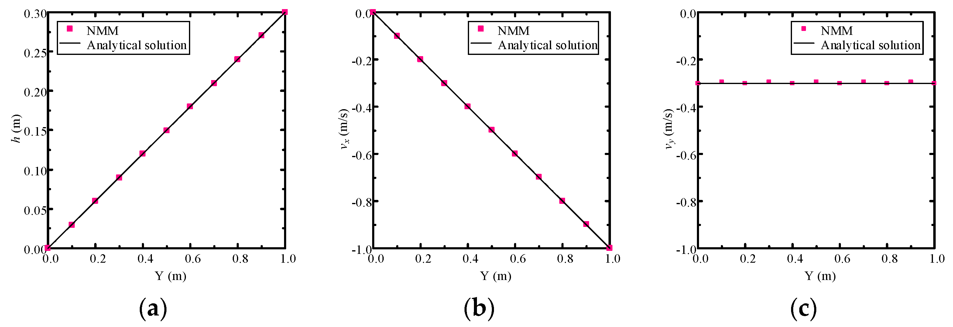
4.1. Example 1: Verification of Homogeneous Darcy Flow with an Analytical Solution

In order to verify the accuracy for a Darcy flow simulation before modeling heterogeneous problems, a homogeneous model is studied. As shown in Figure 6a, a $1\times 1\mathrm{m}$ rectangular domain with Dirichlet boundary conditions is as follows: $h\left(0,y\right)=0$, $h\left(x,0\right)=0$, $h\left(1,y\right)=y$, and $h\left(x,1\right)=x$. The model is homogeneous and isotropic with a permeability coefficient of $k\left(x,y\right)=1\mathrm{m}/\mathrm{s}$. The analytical solution of the hydraulic head is $h\left(x,y\right)=xy$. Thus, the Darcy velocity can be derived by Darcy’s law or Equation (6) as follows: $v_x=-k_x\frac{\partial h}{\partial x}=-y$, $v_y=-k_y\frac{\partial h}{\partial y}=-x$.

The numerical results solved by the proposed method with a 10-layers mesh are shown in Figure 7. Figure 7a shows the distribution of the hydraulic head in the problem domain, and Figure 7b,c are the distributions of the Darcy velocity component $v_x$ and $v_y$, respectively. It is obvious that the hydraulic head and Darcy velocity are both continuous in the problem domain. To realize the advanced feature of the new model, a contrast simulation using the conventional NMM model is studied. Figure 8a is the result of the hydraulic head, which is similar to Figure 7a. Compared with the continuous Darcy velocity in Figure 7b,c, the velocity field obtained though the conventional model is discontinuous both around nodes and across element edges (Figure 8b,c). Therefore, it is proven that the proposed NMM model can achieve a continuous nodal velocity.

Since the analytical solution is known in this problem, we can compare the numerical result with its exact result. Figure 9a shows the comparison of the hydraulic head solution along a profile located at x = 0.3 m, and Figure 9b,c are the comparison of the Darcy velocity component $v_x$ and $v_y$, respectively. It is indicated that the accuracy of the new NMM model is close to the analytical solution without a refined mesh.

Furthermore, in order to analyse the accuracy and convergence of the numerical solution, the relative error of the hydraulic head in the L² norm can be written as

$${\eta }_h=\frac{{\left[{{\displaystyle \int }}_{\mathsf{\Omega }}^{}{\left(h-\widehat{h}\right)}^2\mathrm{d}\mathsf{\Omega }\right]}^{\frac{1}{2}}}{{\left[{{\displaystyle \int }}_{\mathsf{\Omega }}^{}{\widehat{h}}^2\mathrm{d}\mathsf{\Omega }\right]}^{\frac{1}{2}}}\times 100\%$$

(42)

where $h$ is the numerical solution of the hydraulic head and $\widehat{h}$ is the analytical solution. Similarly, the relative error of the Darcy velocity in the L² norm is defined as

$${\eta }_v=\frac{{\left[{{\displaystyle \int }}_{\mathsf{\Omega }}^{}{\left(\mathit{v}-\widehat{\mathit{v}}\right)}^{\mathrm{T}}·\left(\mathit{v}-\widehat{\mathit{v}}\right)\mathrm{d}\mathsf{\Omega }\right]}^{\frac{1}{2}}}{{\left[{{\displaystyle \int }}_{\mathsf{\Omega }}^{}{\widehat{\mathit{v}}}^{\mathrm{T}}·\widehat{\mathit{v}}\mathrm{d}\mathsf{\Omega }\right]}^{\frac{1}{2}}}\times 100\%$$

(43)

where $\mathit{v}$ is the numerical solution of the Darcy velocity and $\widehat{\mathit{v}}$ is the analytical solution.

After convergence analysis for both the new NMM model and the conventional NMM model, the convergence curves of the hydraulic head and Darcy velocity are plotted in Figure 10a,b, respectively. As shown in Figure 10a, the two curves are almost coincident, indicating that they have the same accuracy and convergence rate for the solution of the hydraulic head. However, Figure 10b shows that the velocity solution of the new NMM model is more accurate than the convention NMM model, and their convergence rates are still the same. The values of relative error and convergence rate of both hydraulic head and Darcy velocity by the two NMM models are shown in

Table 1. Error in the L² norm of hydraulic head and Darcy velocity by the proposed NMM model.

kh 1	L2 Error of Hydraulic Head		L2 Error of Darcy Velocity
	Relative Error	Convergence Rate	Relative Error	Convergence Rate
5	2.18 × 10−3	–	4.84 × 10−2	–
10	5.47 × 10−4	−1.10	2.42 × 10−2	−0.55
15	2.44 × 10−4	−1.06	1.61 × 10−2	−0.53
20	1.29 × 10−4	−1.04	1.19 × 10−2	−0.50
25	8.36 × 10−5	−1.03	9.55 × 10−3	−0.52
30	5.86 × 10−5	−1.02	7.98 × 10−3	−0.52

¹ kh means the half number of mesh layers in the vertical direction.

and

Table 2. Error in the L² norm of hydraulic head and Darcy velocity by the convention NMM model.

kh	L2 Error of Hydraulic Head		L2 Error of Darcy Velocity
	Relative Error	Convergence Rate	Relative Error	Convergence Rate
5	2.05 × 10−3	–	6.07 × 10−2	–
10	5.14 × 10−4	−1.10	3.04 × 10−2	−0.55
15	2.29 × 10−4	−1.06	2.03 × 10−2	−0.53
20	1.21 × 10−4	−1.04	1.49 × 10−2	−0.50
25	7.84 × 10−5	−1.03	1.20 × 10−2	−0.52
30	5.49 × 10−5	−1.02	1.00 × 10−2	−0.52

, respectively.

To demonstrate the capability of handling complex boundaries by the proposed method, the same model with a quadratic Dirichlet boundary condition is simulated, as shown in Figure 6b. The boundary conditions are $h\left(0,y\right)=0$, $h\left(x,0\right)=0$, $h\left(1,y\right)=y^2$, and $h\left(x,1\right)=x$, and the permeability coefficient remains unchanged. Note that the source term in this model is $Q=2x$. The analytical solutions of the hydraulic head and Darcy velocity are $h\left(x,y\right)=x{y}^2$, $v_x=-y^2$, and $v_y=-2xy$, respectively.

First, the problem is simulated by the proposed NMM model with a 60-layers mesh. As shown in Figure 11, the distributions of the hydraulic head and Darcy velocity are presented. From Figure 11a, an obvious difference in hydraulic head distribution caused by the change of boundary conditions can be observed compared to Figure 8a. Furthermore, the velocity field is also continuous in the problem domain (Figure 11b,c).

By using different mesh densities, the accuracy of the proposed method for complex boundary conditions is verified. As shown in Figure 12a, the hydraulic head solution along a profile located at x = 0.3 m, in spite of different mesh densities, almost achieves its analytical solution. The Darcy velocity solution is also reliable compared with its analytical result (Figure 12b,c). In addition, when the mesh density reaches 60 layers, the Darcy velocity solution almost achieves its analytical solution.

Convergence analysis is performed both for hydraulic heads and velocities. Figure 13a shows the convergence curve of the hydraulic head, and Figure 13b shows the convergence curve of the Darcy velocity. However, there is no big difference with Figure 10, except that the relative errors of both the hydraulic head and Darcy velocity are larger than last examples, since the problem has more complex boundary conditions.

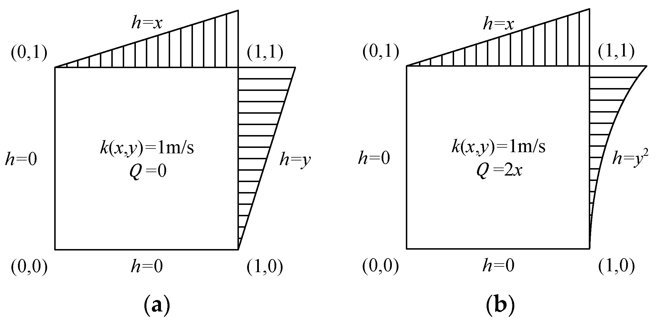
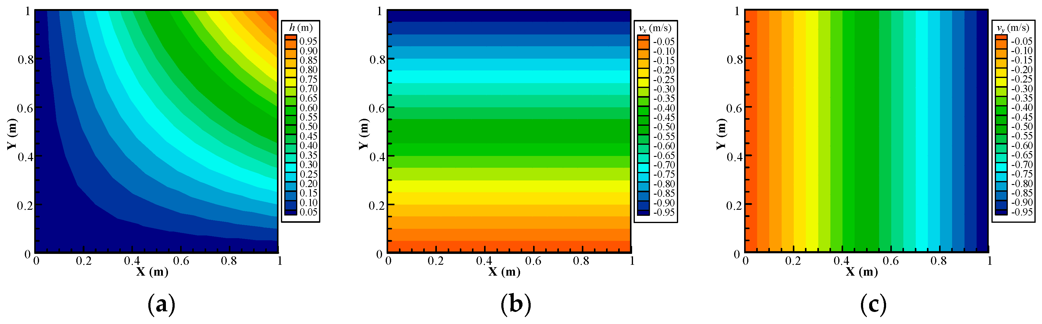
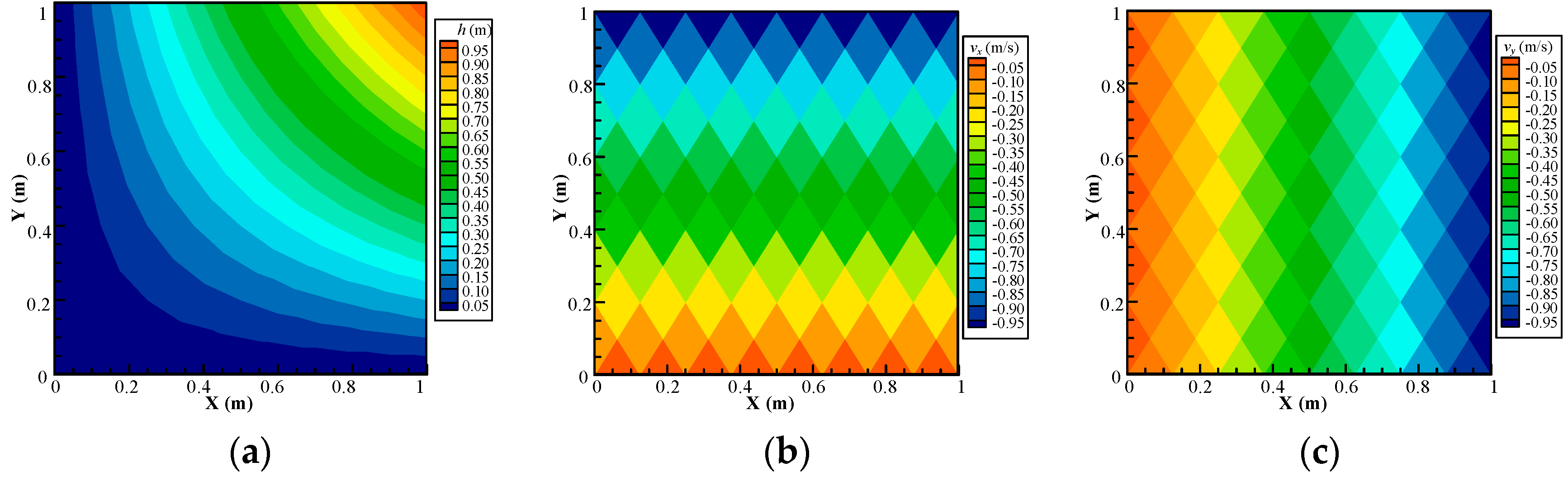
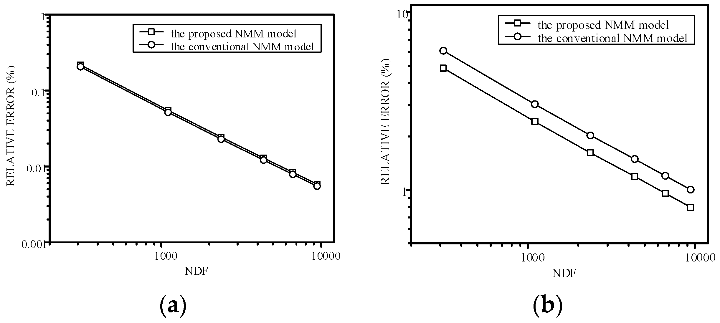
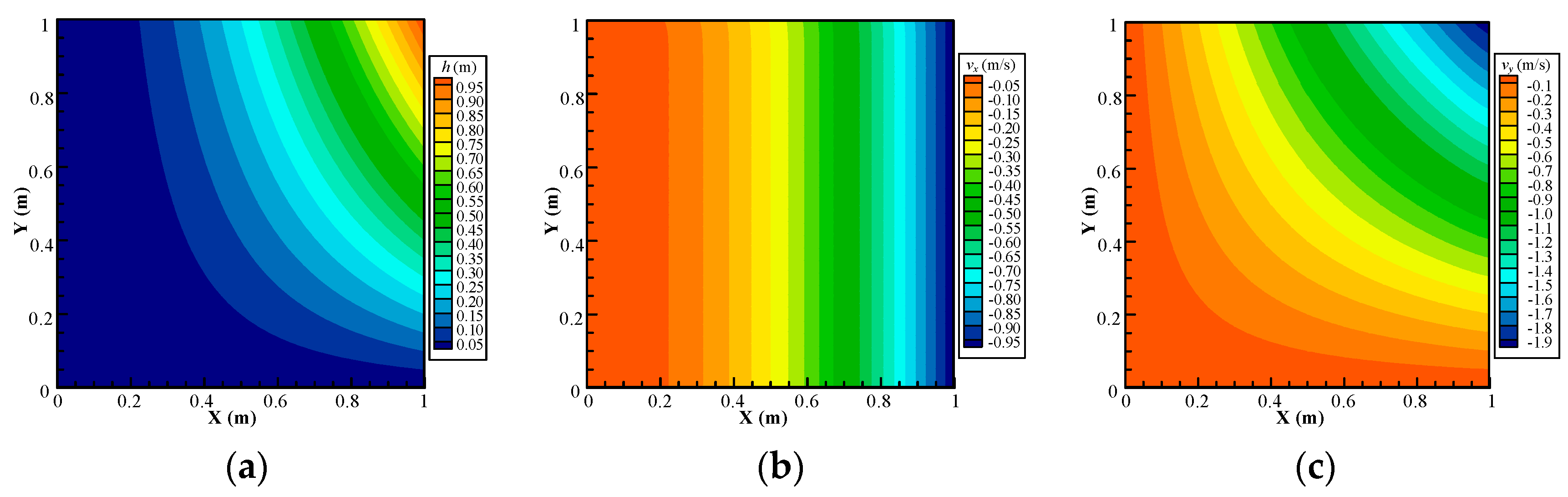
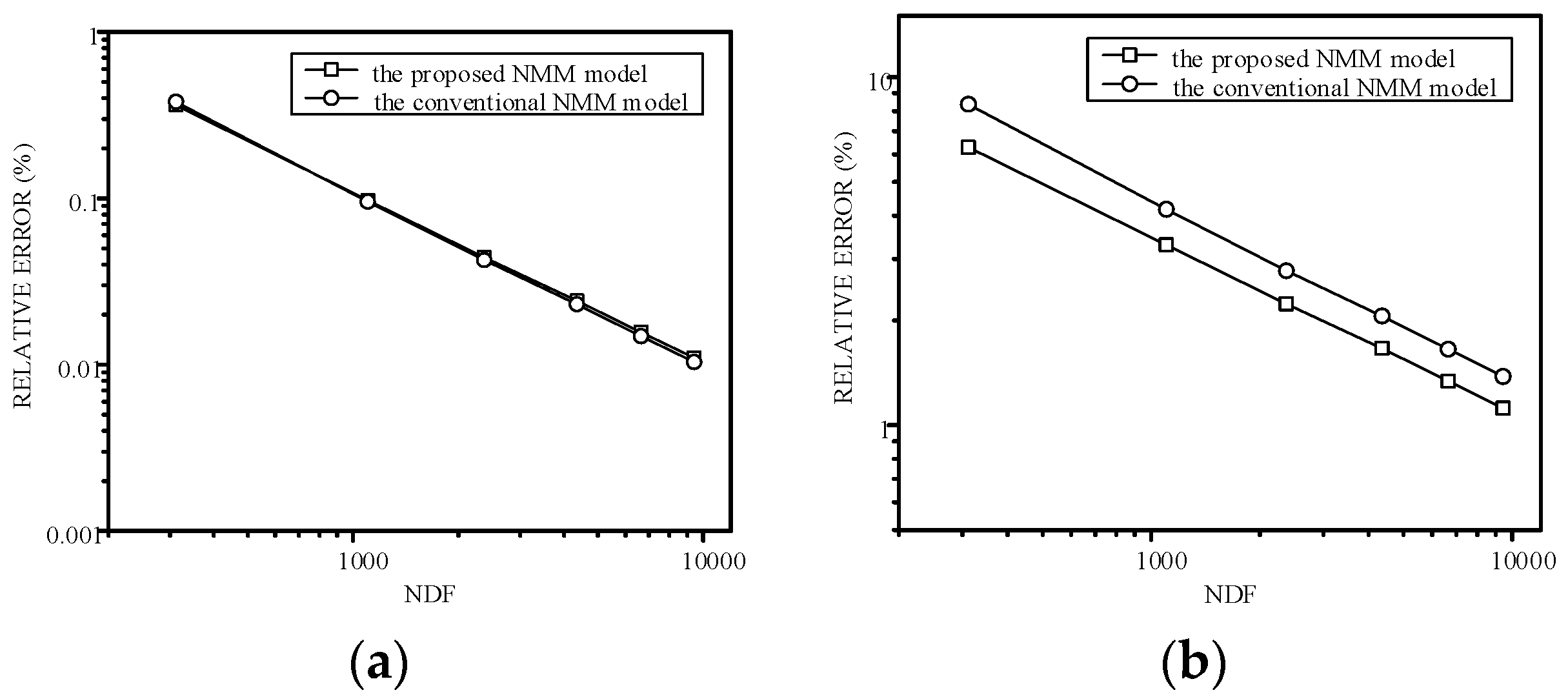
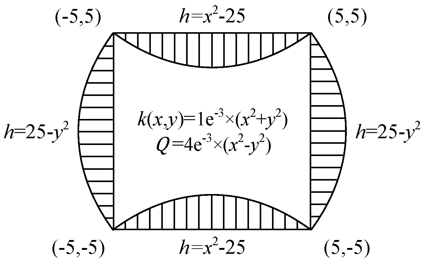
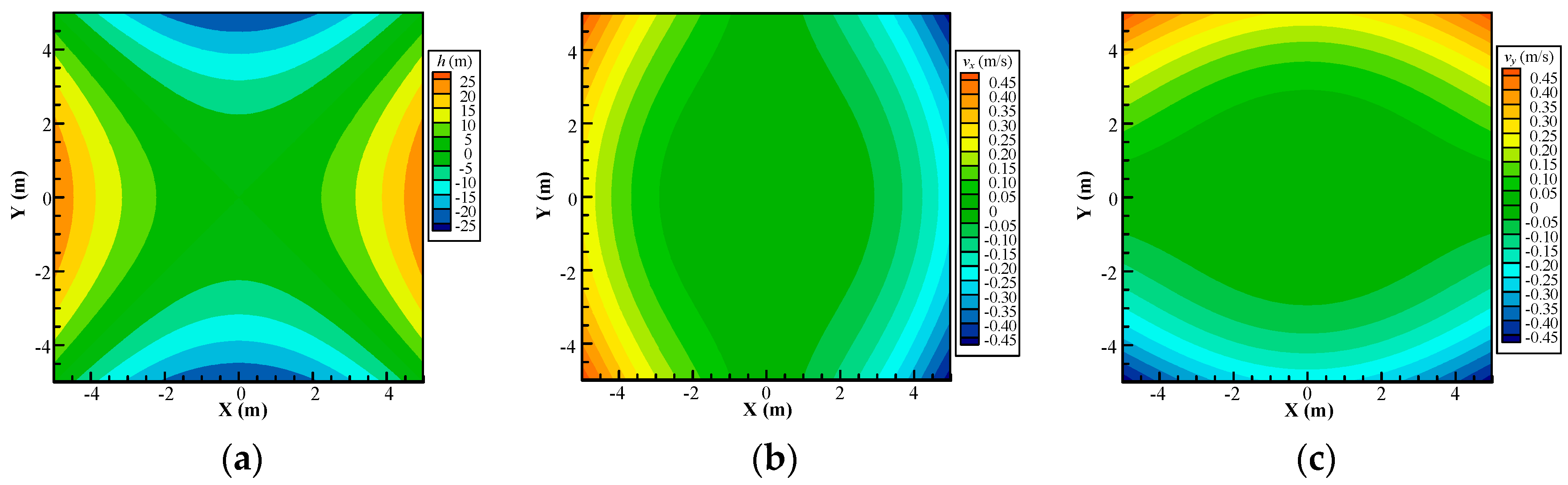
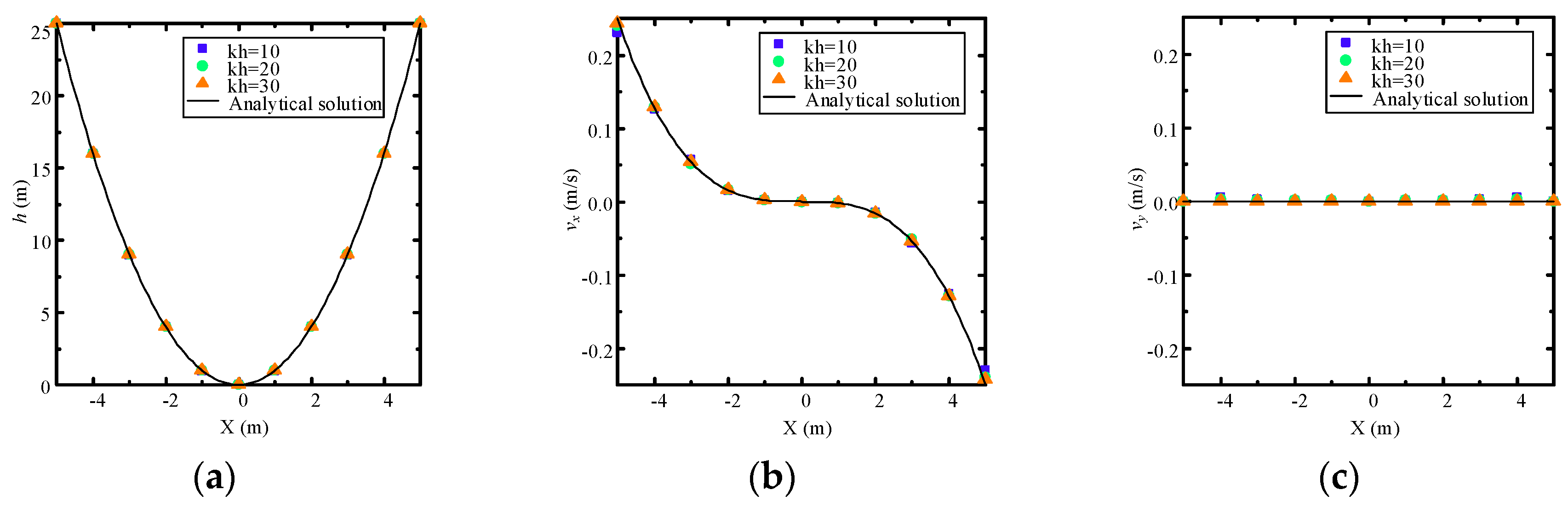
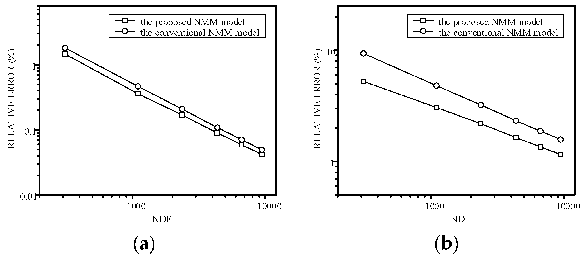
4.2. Example 2: Accuracy Darcy Velocity Solution for Continuous-Heterogeneous Media

A continuous-heterogeneous model, as shown in Figure 14, is simulated in this example. The boundary conditions are as follows: $h\left(x,-5\right)=h\left(x,5\right)=x^2-25$ and $h\left(-5,y\right)=h\left(5,y\right)=25-y^2$. The hydraulic conductivity varies smoothly within the problem domain, expressed as $\mathrm{k}\left(x,y\right)=1{\mathrm{e}}^{-3}\times \left(x^2+y^2\right)$. In addition, a source term $Q=4{\mathrm{e}}^{-3}\times \left(x^2-y^2\right)$, is included in this model. The analytical solution of hydraulic head is $h\left(x,y\right)=x^2-y^2$, and the solution of the velocity field can be derived as $v_x=-2{\mathrm{e}}^{-3}\times \left(x^3+x{y}^2\right)$ and $v_y=2{\mathrm{e}}^{-3}\times \left(x^{2}y+y^3\right)$.

Figure 15a shows the distribution of hydraulic head, whereas Figure 15b,c show the distribution of the Darcy velocity $v_x$ and $v_y$, respectively. The contour plots show that the distribution of numerical results is symmetric and continuous by the proposed model. In order to study the robustness of the cover system, numerical results along a profile at y = 0 m with 20, 40, and 60 layers of mesh are compared with the analytical solution. Figure 16a shows the comparison of the hydraulic head solution between the proposed NMM model and the analytical solution along a profile located at y = 0 m, indicating high precision for the hydraulic head solution. Furthermore, the Darcy velocity solution also shows good agreement with the analytical solution in this continuous-heterogeneous media in Figure 16b,c.

For this continuous-heterogeneous problem, convergence curves of both the hydraulic head and velocity are shown in Figure 17. According to Figure 17a, the hydraulic head solution found using the proposed NMM model is more accurate than that of the conventional NMM model, and the convergence rate is still the same. Moreover, the proposed high-order NMM model also shows better accuracy of the Darcy velocity solution than the conventional model, while their convergence rates are almost the same.

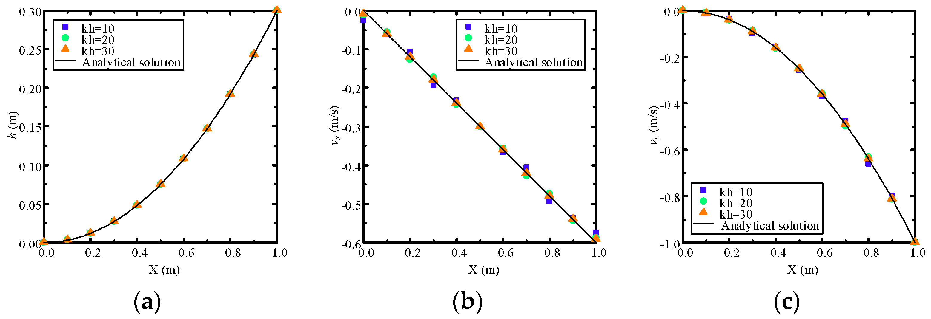
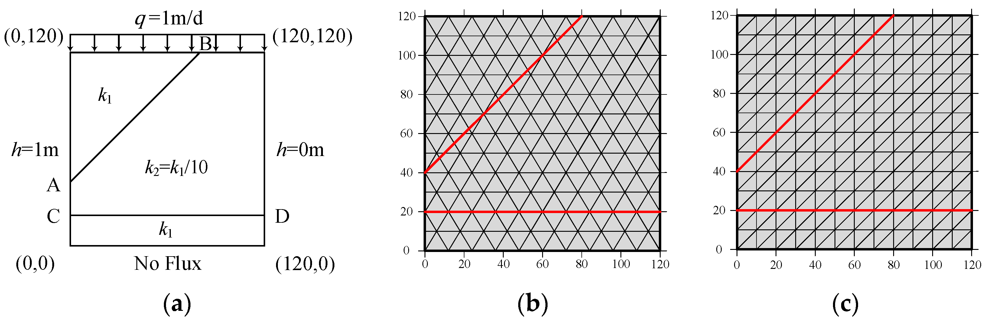
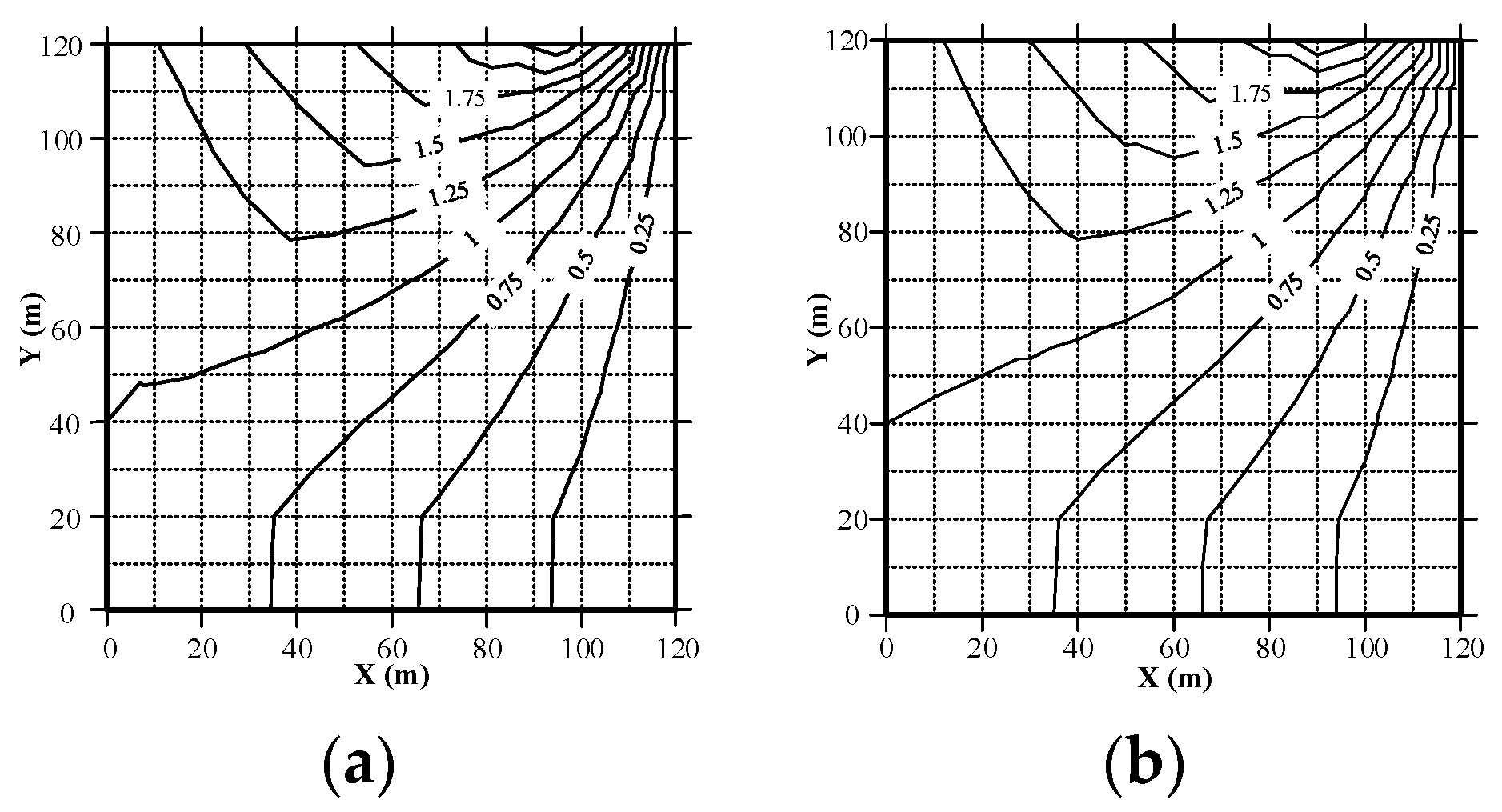
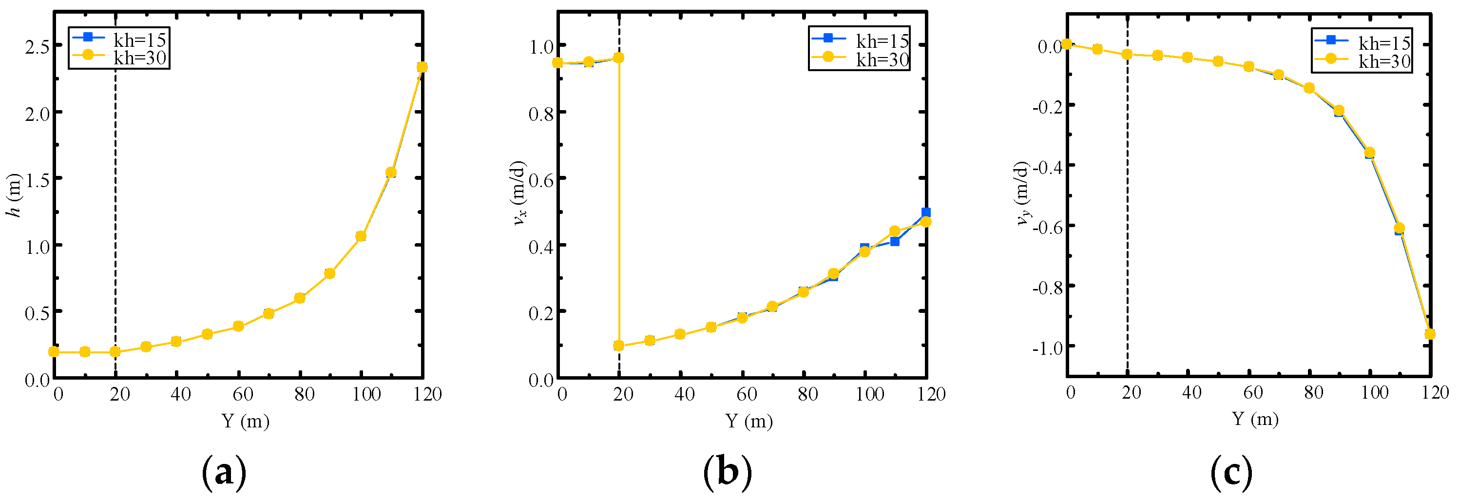
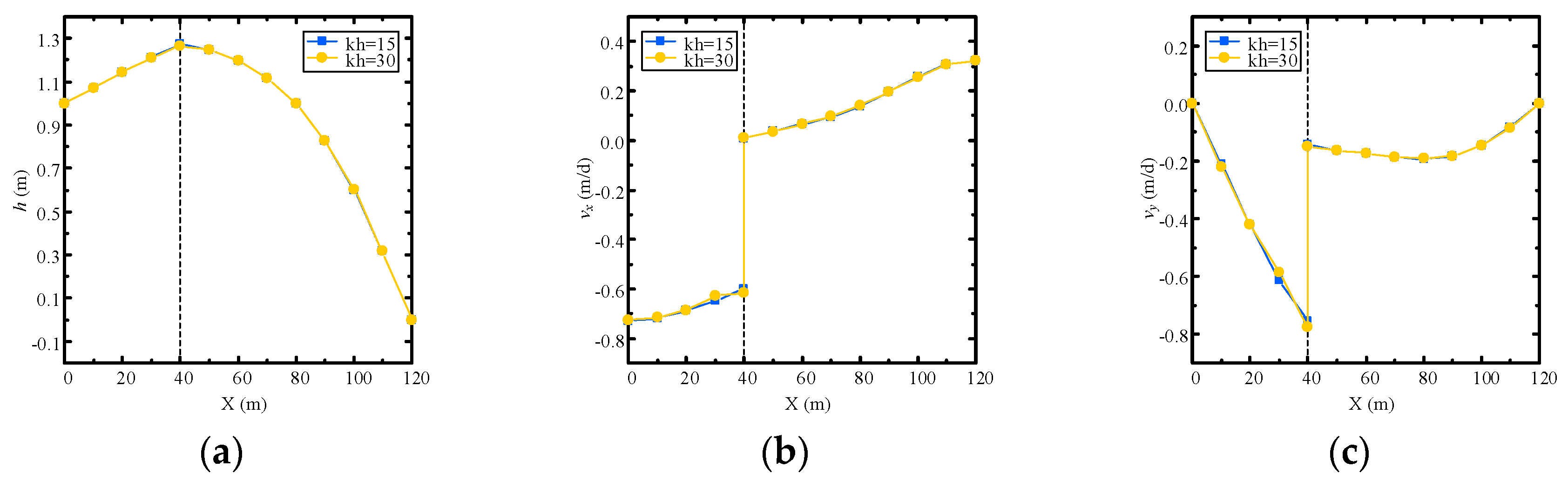
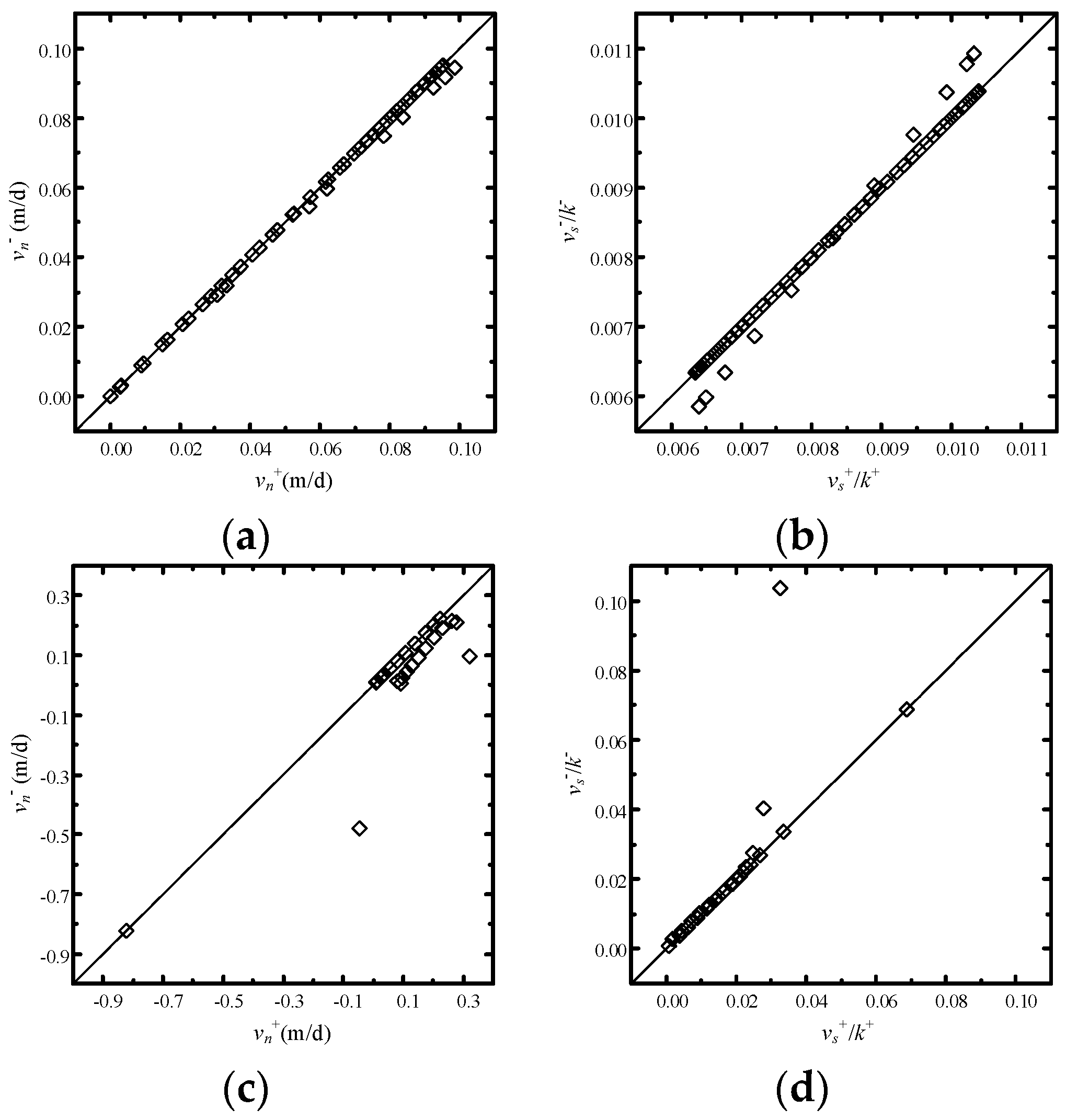
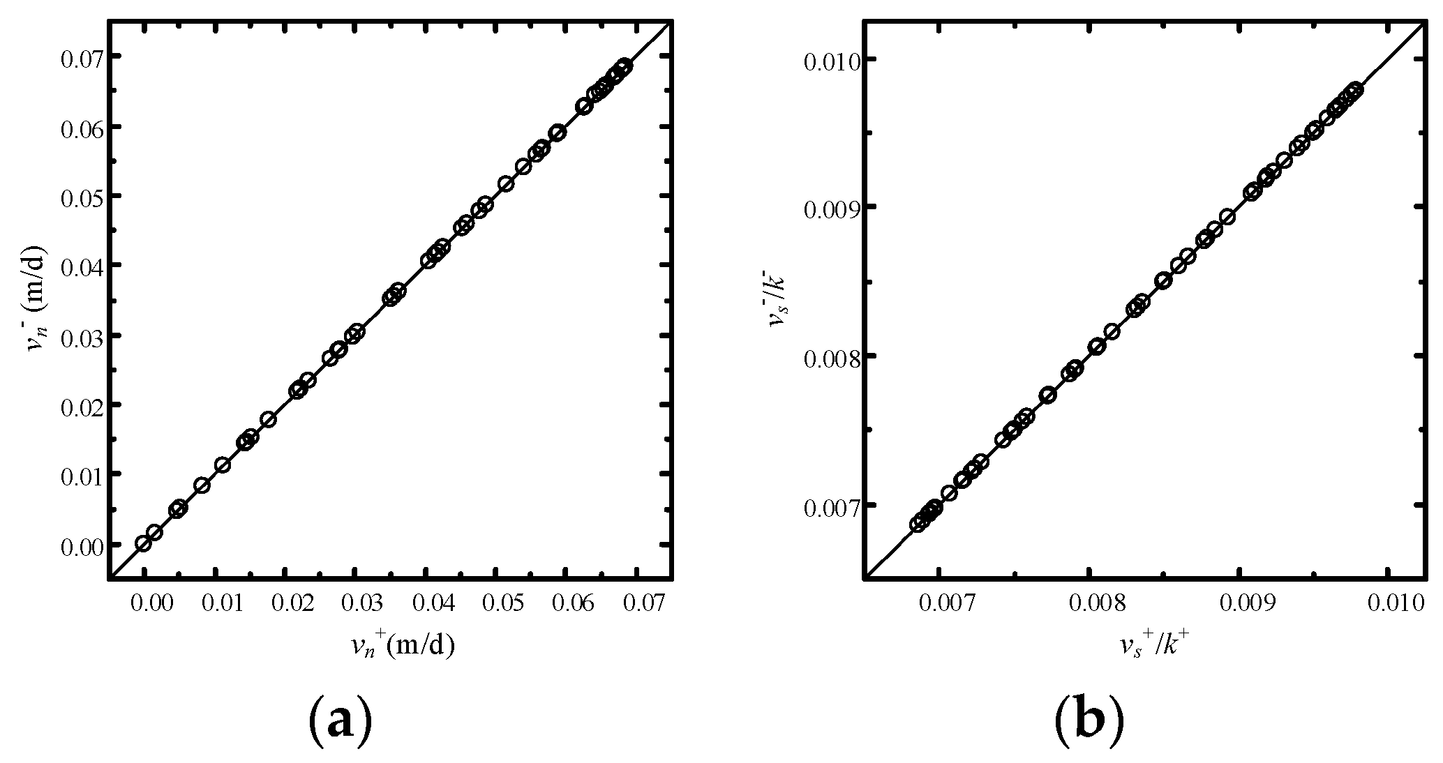
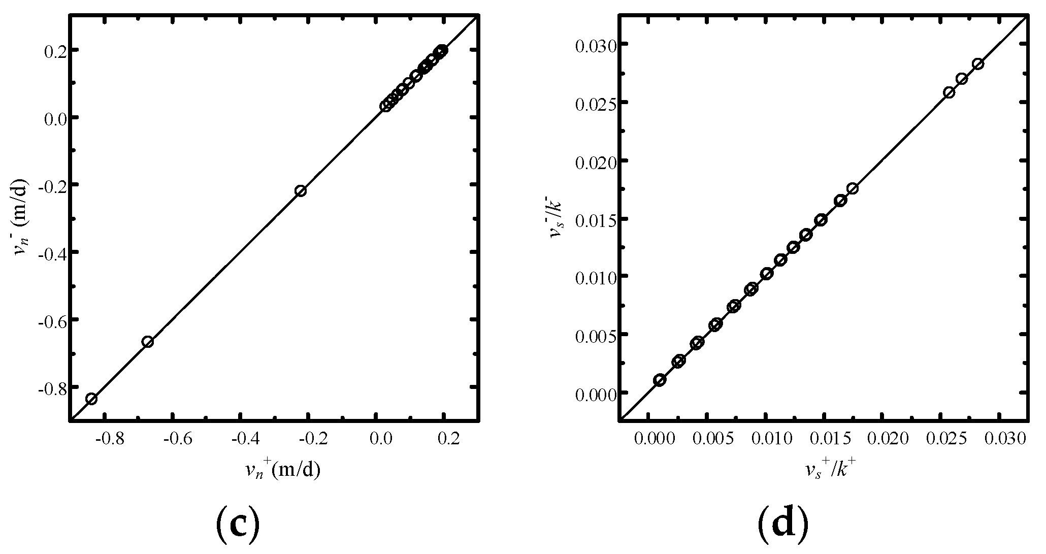
4.3. Example 3: Verification of Refraction Law for Discontinuous-Heterogeneous Media

The last example is to verify the refraction law across material interfaces [14], as shown in Figure 18a. Considering a rectangular domain of 120 × 120 m with material interfaces AB and CD, the permeability coefficients are $k_1=100\mathrm{m}/\mathrm{d}$ and $k_2=10\mathrm{m}/\mathrm{d}$, respectively. The hydraulic heads are fixed with 1 m on the left side and 0 m on the right side, while the top boundary has a specified inflow flux of $q=1\mathrm{m}/\mathrm{d}$. The bottom of the model is impermeable. Due to the dual cover systems, the NMM mesh (Figure 18b) does not need to conform with the material interfaces, unlike the conventional FEM mesh (Figure 18c).

The comparison of the hydraulic head distribution simulated by the proposed NMM model and Zhou’s FEM model with same mesh size is shown in Figure 19. The results show that the hydraulic head is continuous across the material interfaces AB and CD.

In order to study the influence of the material interface, numerical results with two different mesh densities along profiles at x = 100 m and y = 80 m are plotted in Figure 20 and Figure 21. As shown in Figure 20, the hydraulic head across the material interface is continuous, while the Darcy velocity is discontinuous. Similar results are shown by Figure 21, however, the Darcy velocity in the y direction is continuous as the material interface happens to be perpendicular to the y-axis.

For the purpose of verifying the accuracy of modeling refraction law across material interfaces, the velocity components of element nodes on the different sides of the material interface AB are plotted in Figure 22 and Figure 23. The results show that the requirement of the refraction law cannot be strictly met using the conventional NMM model (Figure 22). Thus, the numerical results may be unreliable. As shown in Figure 23, the velocity components solved by the proposed model fully satisfy the refraction law, as well as Zhou’s model [14].

As a result, the proposed NMM model can achieve the same precision of the Darcy velocity as Zhou’s method without iterations, while the dual cover systems of NMM model are more flexible and convenient without the need of conforming to material interfaces. Moreover, the new model is proven to be insensitive to mesh size, so that reliable results can be achieved through a sparse mesh. Therefore, the proposed NMM model is very suitable for modeling the Darcy flow in heterogeneous porous media.

5. Discussion and Conclusions

In this paper, a new high-order NMM model for the Darcy flow in heterogeneous porous media is presented. Due to the lack precision of measuring the velocity solution by ordinary methods, a new weight function with a continuous nodal gradient was adopted into the original NMM model. In order to achieve best precision when modeling material interfaces, the refraction law is fully introduced into the NMM model as an a posteriori requirement. Compared to other numerical schemes, the proposed NMM model has three major advantages as follows:

(1)

the solution of Darcy velocity is accurate, and continuous at each node;

(2)

the material interfaces exactly satisfy the refraction law, and thus the simulation results can be accurate and reliable; and

(3)

the pre-processing work is efficient, due to the two independent cover systems of NMM, in contrast with other numerical schemes. Especially for complex heterogeneous problems even with intersecting material interfaces, the proposed model provides a significant advantage.

Additionally, a set of numerical examples are modeled to verify the accuracy, efficiency, and robustness of the proposed high-order numerical manifold method. First, Darcy flow in homogeneous porous media with different boundary conditions is simulated. The numerical results show good precision compared with analytical solutions, which is the foundation for modeling heterogeneous problems. Then, a continuous-heterogeneous example with hydraulic conductivity varying smoothly in the problem domain is demonstrated. Compared with the analytical solution, the developed method shows the ability to model heterogeneous problem without material interfaces. Moreover, convergence analysis shows that the new model has better accuracy for the Darcy velocity solution, especially in heterogeneous problems. Finally, the new high-order NMM model is applied into a heterogeneous problem with material interfaces and different boundary conditions. Results show that refraction law is exactly satisfied by the proposed model, while the computational cost, especially the mesh effort, is less than that of the existing models.

Furthermore, the proposed high-order NMM model can be extended to 3D cases and applied into fluid flow and contaminant transportation in heterogeneous porous media.

References

1. Bear, J. Dynamics of Fluids in Porous Media; American Elsevier Publishing Company: New York, NY, USA, 1972. [Google Scholar]
2. Cainelli, O.; Bellin, A.; Putti, M. On the accuracy of classic numerical schemes for modeling flow in saturated heterogeneous formations. Adv. Water Resour. 2012, 47, 43–55. [Google Scholar] [CrossRef]
3. Bellin, A.; Salandin, P.; Rinaldo, A. Simulation of dispersion in heterogeneous porous formations: Statistics, first-order theories, convergence of computations. Water Resour. Res. 1992, 28, 2211–2227. [Google Scholar] [CrossRef]
4. Neuman, S.; Orr, S.; Levin, O.; Paleologos, E. Theory and high-resolution finite element analysis of 2-d and 3-d effective permeabilities in strongly heterogeneous porous media. In Proceedings of the 9th International Conference on Computational Methods in Water Resources, Denver, CO, USA, 1 June 1992. [Google Scholar]
5. Ababou, R.; McLaughlin, D.; Gelhar, L.W.; Tompson, A.F. Numerical simulation of three-dimensional saturated flow in randomly heterogeneous porous media. Transp. Porous Media 1989, 4, 549–565. [Google Scholar] [CrossRef]
6. Chin, D.A.; Wang, T. An investigation of the validity of first-order stochastic dispersion theories in isotropie porous media. Water Resour. Res. 1992, 28, 1531–1542. [Google Scholar] [CrossRef]
7. Tompson, A.F.; Gelhar, L.W. Numerical simulation of solute transport in three-dimensional, randomly heterogeneous porous media. Water Resour. Res. 1990, 26, 2541–2562. [Google Scholar] [CrossRef]
8. Batu, V. A finite element dual mesh method to calculate nodal darcy velocities in nonhomogeneous and anisotropic aquifers. Water Resour. Res. 1984, 20, 1705–1717. [Google Scholar] [CrossRef]
9. Yeh, G.T. On the computation of Darcian velocity and mass balance in finite elements modeling of groundwater flow. Water Resour. Res. 1981, 17, 1529–1534. [Google Scholar] [CrossRef]
10. Zhang, Z.; Xue, Y.; Wu, J. A cubic-spline technique to calculate nodal Darcian velocities in aquifers. Water Resour. Res. 1994, 30, 975–981. [Google Scholar] [CrossRef]
11. D’Angelo, C.; Scotti, A. A mixed finite element method for darcy flow in fractured porous media with non-matching grids. ESAIM-Math 2012, 46, 465–489. [Google Scholar] [CrossRef]
12. Masud, A.; Hughes, T.J.R. A stabilized mixed finite element method for darcy flow. Comput. Meth. Appl. Mech. Eng. 2002, 191, 4341–4370. [Google Scholar] [CrossRef]
13. Mosé, R.; Siegel, P.; Ackerer, P.; Chavent, G. Application of the mixed hybrid finite element approximation in a groundwater flow model: Luxury or necessity? Water Resour. Res. 1994, 30, 3001–3012. [Google Scholar] [CrossRef]
14. Zhou, Q.; Bensabat, J.; Bear, J. Accurate calculation of specific discharge in heterogeneous porous media. Water Resour. Res. 2001, 37, 3057–3069. [Google Scholar] [CrossRef] [Green Version]
15. Xie, Y.F.; Wu, J.C.; Xue, Y.Q.; Xie, C.H.; Ji, H.F. A domain decomposed finite element method for solving darcian velocity in heterogeneous porous media. J. Hydrol. 2017, 554, 32–49. [Google Scholar] [CrossRef]
16. Shi, G.H. Manifold method of material analysis. In Proceedings of the Transactions of the 9th Army Conference on Applied Mathematics and Computing, Minneapolis, MN, USA, 18–21 June 1991; pp. 57–76. [Google Scholar]
17. Shi, G.H. Modeling rock joints and blocks by manifold method. In Proceedings of the 33th U.S. Symposium on Rock Mechanics, Santa Fe, NM, USA, 3–5 June 1992; pp. 639–648. [Google Scholar]
18. Ma, G.W.; An, X.M.; Zhang, H.H.; Li, L.X. Modeling complex crack problems using the numerical manifold method. Int. J. Fract. 2009, 156, 21–35. [Google Scholar] [CrossRef]
19. Zhang, H.H.; Li, L.X.; An, X.M.; Ma, G.W. Numerical analysis of 2-d crack propagation problems using the numerical manifold method. Eng. Anal. Bound. Elem. 2010, 34, 41–50. [Google Scholar] [CrossRef]
20. Wu, Z.J.; Wong, L.N.Y. Frictional crack initiation and propagation analysis using the numerical manifold method. Comput. Geotech. 2012, 39, 38–53. [Google Scholar] [CrossRef]
21. Zheng, H.; Xu, D.D. New strategies for some issues of numerical manifold method in simulation of crack propagation. Int. J. Numer. Methods Eng. 2014, 97, 986–1010. [Google Scholar] [CrossRef] [Green Version]
22. Ning, Y.J.; An, X.M.; Ma, G.W. Footwall slope stability analysis with the numerical manifold method. Int. J. Rock Mech. Min. Sci. 2011, 48, 964–975. [Google Scholar] [CrossRef]
23. He, L.; An, X.M.; Ma, G.W.; Zhao, Z.Y. Development of three-dimensional numerical manifold method for jointed rock slope stability analysis. Int. J. Rock Mech. Min. Sci. 2013, 64, 22–35. [Google Scholar] [CrossRef]
24. An, X.M.; Ning, Y.J.; Ma, G.W.; He, L. Modeling progressive failures in rock slopes with non-persistent joints using the numerical manifold method. Int. J. Numer. Anal. Methods Geomech. 2014, 38, 679–701. [Google Scholar] [CrossRef]
25. Fan, L.F.; Yi, X.W.; Ma, G.W. Numerical manifold method (NMM) simulation of stress wave propagation through fractured rock mass. Int. J. Appl. Mech. 2013, 5, 20. [Google Scholar] [CrossRef]
26. Wu, Z.J.; Wong, L.N.Y.; Fan, L.F. Dynamic study on fracture problems in viscoelastic sedimentary rocks using the numerical manifold method. Rock Mech. Rock Eng. 2013, 46, 1415–1427. [Google Scholar] [CrossRef]
27. Wong, L.N.Y.; Wu, Z.J. Application of the numerical manifold method to model progressive failure in rock slopes. Eng. Fract. Mech. 2014, 119, 1–20. [Google Scholar] [CrossRef]
28. Zhao, G.F.; Zhao, X.B.; Zhu, J.B. Application of the numerical manifold method for stress wave propagation across rock masses. Int. J. Numer. Anal. Methods Geomech. 2014, 38, 92–110. [Google Scholar] [CrossRef]
29. Ohnishi, Y.; Tanaka, M.; Koyama, T.; Mutoh, K. Manifold method in saturated-unsaturated unsteady groundwater flow analysis. In Proceedings of the Third International Conference on Analysis of Discontinuous Deformation (ICADD-3), Vail, CO, USA, 3–4 June 1999; pp. 221–230. [Google Scholar]
30. Zhang, Z.R.; Zhang, X.W.; Yan, J.H. Manifold method coupled velocity and pressure for navier-stokes equations and direct numerical solution of unsteady incompressible viscous flow. Comput. Fluids 2010, 39, 1353–1365. [Google Scholar] [CrossRef]
31. Jiang, Q.H.; Deng, S.S.; Zhou, C.B.; Lu, W.B. Modeling unconfined seepage flow using three-dimensional numerical manifold method. J. Hydrodyn. 2010, 22, 554–561. [Google Scholar] [CrossRef]
32. Wang, Y.; Hu, M.S.; Zhou, Q.L.; Rutqvist, J. Energy-work-based numerical manifold seepage analysis with an efficient scheme to locate the phreatic surface. Int. J. Numer. Anal. Methods Geomech. 2014, 38, 1633–1650. [Google Scholar] [CrossRef]
33. Hu, M.S.; Wang, Y.; Rutqvist, J. On continuous and discontinuous approaches for modeling groundwater flow in heterogeneous media using the numerical manifold method: Model development and comparison. Adv. Water Resour. 2015, 80, 17–29. [Google Scholar] [CrossRef]
34. Hu, M.S.; Wang, Y.; Rutqvist, J. An effective approach for modeling fluid flow in heterogeneous media using numerical manifold method. Int. J. Numer. Methods Fluids 2015, 77, 459–476. [Google Scholar] [CrossRef]
35. Hu, M.S.; Wang, Y.; Rutqvist, J. Development of a discontinuous approach for modeling fluid flow in heterogeneous media using the numerical manifold method. Int. J. Numer. Anal. Methods Geomech. 2015, 39, 1932–1952. [Google Scholar] [CrossRef]
36. Zheng, H.; Liu, F.; Li, C.G. Primal mixed solution to unconfined seepage flow in porous media with numerical manifold method. Appl. Math. Model. 2015, 39, 794–808. [Google Scholar] [CrossRef]
37. Yang, Y.T.; Zheng, H. A three-node triangular element fitted to numerical manifold method with continuous nodal stress for crack analysis. Eng. Fract. Mech. 2016, 162, 51–75. [Google Scholar] [CrossRef]
38. Yang, Y.T.; Xu, D.D.; Sun, G.H.; Zheng, H. Modeling complex crack problems using the three-node triangular element fitted to numerical manifold method with continuous nodal stress. Sci. China Technol. Sci. 2017, 60, 1537–1547. [Google Scholar] [CrossRef]
39. Zienkiewicz, O.C.; Taylor, R.L.; Zhu, J.Z. The Finite Element Method: Its Basis and Fundamentals, 7th ed.; Butterworth-Heinemann: Oxford, UK, 2013. [Google Scholar]
Figure 1. Finite element mesh and physical domain.
Processes 06 00111 g001
Figure 2. The dual cover systems: mathematical covers and physical covers.
Processes 06 00111 g002
Figure 3. Manifold elements generated by physical covers.
Processes 06 00111 g003
Figure 4. Physical domain and boundaries of a Darcy flow problem.
Processes 06 00111 g004
Figure 5. Refraction law across the material interface.
Processes 06 00111 g005
Figure 6. A 1 × 1   m rectangular model for homogeneous Darcy flow with different boundary conditions: (a) h ( 0 , y ) = 0 , h ( x , 0 ) = 0 , h ( 1 , y ) = y , h ( x , 1 ) = x ; (b) h ( 0 , y ) = 0 , h ( x , 0 ) = 0 , h ( 1 , y ) = y 2 , h ( x , 1 ) = x .
Processes 06 00111 g006
Figure 7. Computed contour map of the (a) hydraulic head, (b) Darcy velocity component in the x direction, and (c) Darcy velocity component in the y direction using the proposed NMM model with a 10-layer mesh.
Processes 06 00111 g007
Figure 8. Computed contour map of the (a) hydraulic head, (b) Darcy velocity component in the x direction, (c) Darcy velocity component in the y direction using the conventional NMM model with a 10-layer mesh.
Processes 06 00111 g008
Figure 9. The comparison of solutions computed by the proposed numerical manifold method (NMM) model using a 10-layer mesh with an analytical solution along a profile located at x = 0.3 m: the (a) hydraulic head, (b) Darcy velocity in the x direction, and (c) Darcy velocity in the y direction.
Processes 06 00111 g009
Figure 10. The comparison of convergence curves in the L2 norm by the proposed NMM model and the conventional NMM model: (a) the relative error of the hydraulic head and (b) the relative error of the Darcy velocity. (NDF: number of degrees of freedom).
Processes 06 00111 g010
Figure 11. Computed contour map of the (a) hydraulic head, (b) Darcy velocity component in the x direction, and (c) Darcy velocity component in the y direction using the conventional NMM model with a 60-layers mesh.
Processes 06 00111 g011
Figure 12. The comparison of solutions computed by the proposed NMM model using different mesh densities with an analytical solution along a profile located at x = 0.3 m: the (a) hydraulic head, (b) Darcy velocity in the x direction, and (c) Darcy velocity in the y direction.
Processes 06 00111 g012
Figure 13. The comparison of convergence curves in the L2 norm by the proposed NMM model and the conventional NMM model: (a) the relative error of the hydraulic head and (b) the relative error of the Darcy velocity.
Processes 06 00111 g013
Figure 14. A continuous-heterogeneous model for Darcy flow: model geometry and boundary conditions.
Processes 06 00111 g014
Figure 15. Computed contour map of the (a) hydraulic head, (b) Darcy velocity component in the x direction, and (c) Darcy velocity component in the y direction using the proposed NMM model with a 60-layer mesh.
Processes 06 00111 g015
Figure 16. The comparison of solutions computed by the proposed NMM model using different mesh densities with an analytical solution along a profile located at y = 0 m: the (a) hydraulic head, (b) Darcy velocity component in the x direction, and (c) Darcy velocity component in the y direction.
Processes 06 00111 g016
Figure 17. The comparison of convergence curves in the L2 norm by the proposed NMM model and the conventional NMM model: the (a) the relative error of the hydraulic head and (b) the relative error of the Darcy velocity.
Processes 06 00111 g017
Figure 18. A discontinuous-heterogeneous model with material interfaces: (a) model geometry and boundary conditions, (b) non-conforming mesh based on the proposed NMM model, and (c) conforming mesh based on Zhou’s FEM model [14].
Processes 06 00111 g018
Figure 19. Numerical results of hydraulic head distribution simulated by (a) the proposed NMM model and (b) Zhou’s FEM model [14].
Processes 06 00111 g019
Figure 20. The comparison of solutions computed by the proposed NMM model using different mesh densities with an analytical solution along a profile located at x = 100 m: the (a) hydraulic head, (b) Darcy velocity component in the x direction, and (c) Darcy velocity component in the y direction.
Processes 06 00111 g020
Figure 21. The comparison of solutions computed by the proposed NMM model using different mesh densities with an analytical solution along a profile located at y = 80 m: the (a) hydraulic head, (b) Darcy velocity component in the x direction, and (c) Darcy velocity component in the y direction.
Processes 06 00111 g021
Figure 22. Verification of the refraction law on the material interface using the conventional NMM model: the (a) normal component on AB, (b) tangential component on AB, (c) normal component on CD, and (d) tangential component on CD.
Processes 06 00111 g022
Figure 23. Verification of the refraction law on the material interface using the conventional NMM model: the (a) normal component on AB, (b) tangential component on AB, (c) normal component on CD, and (d) tangential component on CD.
Processes 06 00111 g023aProcesses 06 00111 g023b