Parameter Identification For Continuous Fluidized Bed Spray Agglomeration

Abstract

Agglomeration represents an important particle formation process used in many industries. One particularly attractive process setup is continuous fluidized bed spray agglomeration, which features good mixing as well as high heat and mass transfer on the one hand and constant product throughput with constant quality as well as high flow rates compared to batch mode on the other hand. Particle properties such as agglomerate size or porosity significantly affect overall product properties such as re-hydration behavior and dissolubility. These can be influenced by different operating parameters. In this manuscript, a population balance model for a continuous fluidized bed spray agglomeration is presented and adapted to experimental data. Focus is on the description of the dynamic behavior in continuous operation mode in a certain neighborhood around steady-state. Different kernel candidates are evaluated and it is shown that none of the kernels are able to match the first six minutes with time independent parameters. Afterwards, a good fit can be obtained, where the Brownian and the volume independent kernel models match best with the experimental data. Model fit is improved for identification on a shifted time domain neglecting the initial start-up phase. Here, model identifiability is shown and parameter confidence intervals are computed via parametric bootstrap.

1. Introduction

Agglomeration is a particle formation process in which at least two primary particles are combined to form a new one. This principle is often used in many industries, e.g., pharmaceutical manufacturing and food processing. The properties of the formed agglomerates, e.g., size, shape and porosity, significantly affect its end-use properties, e.g., dissolubility of food powders, processability and storeability [1]. In industrial practice, agglomerates are often formed in drums, pans or fluidized beds. The advantages of the latter include good mixing as well as high heat and mass transfer between particles, liquid and gas phase [2]. Compared to widely applied batch processes, an additional benefit of operating in continuous mode is a constant throughput with constant quality due to the steady-state operation. Therefore, in this contribution the focus is on continuous fluidized bed spray agglomeration, which was not in the focus of research efforts so far.

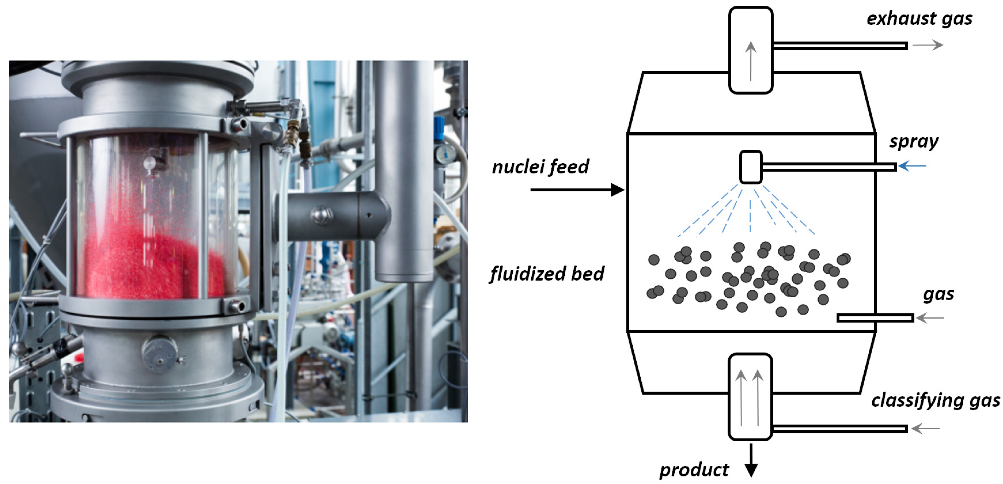
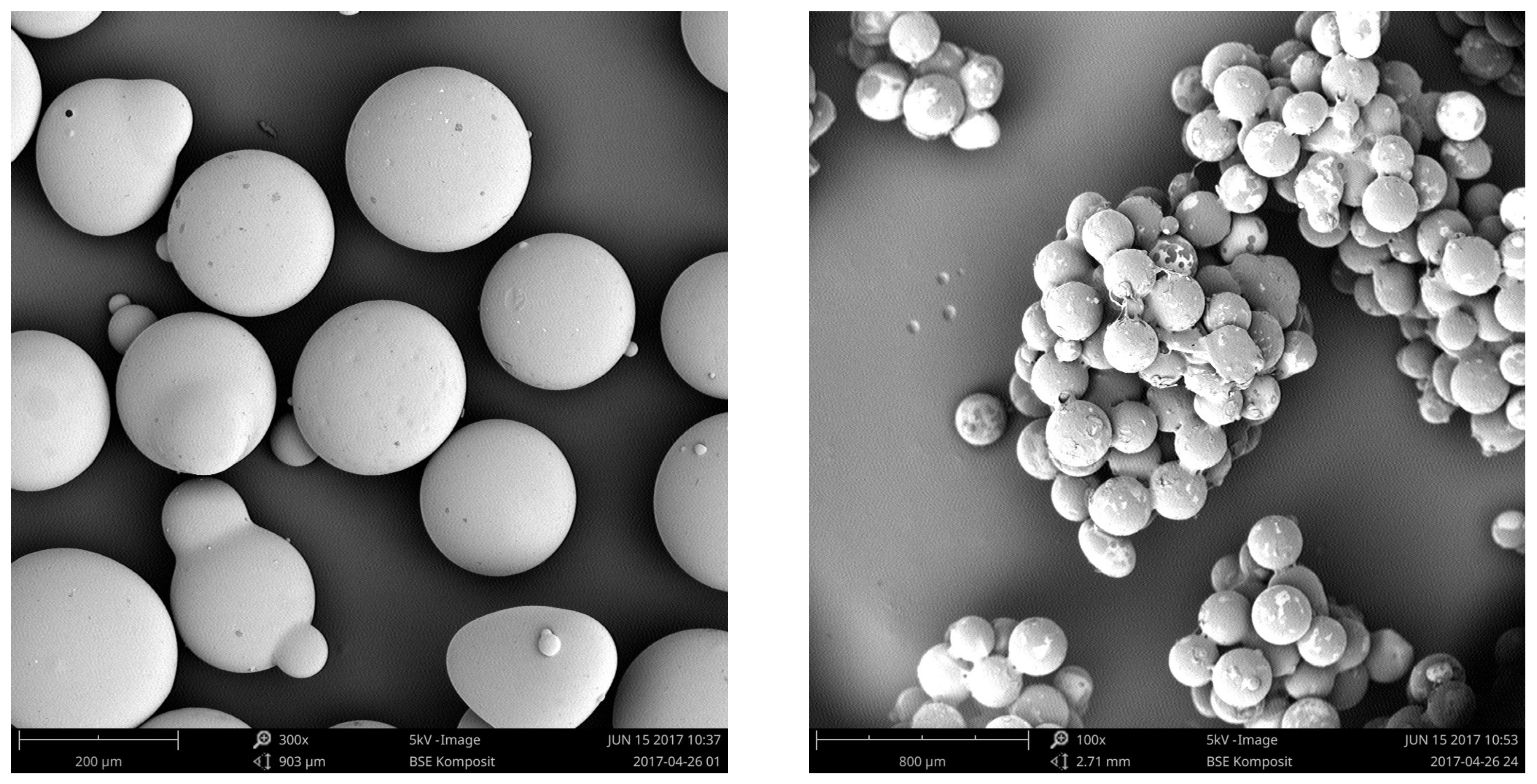
The process scheme is shown in Figure 1. The particles in the chamber are fluidized by a flow of hot gas from the bottom, liquid binder is sprayed on the particles in the form of small droplets to make them wet. Due to random collisions liquid bridges between particles are formed. These can become solid by drying and thereby agglomerates consisting of different numbers of individuals are formed. Microscopic pictures of primary particles and agglomerates are depicted in Figure 2.

The formation of the agglomerates and thereby the product properties can be influenced by variation of different operating parameters and process configurations, such as feed rate, binder concentration and temperature of the fluidization gas [3,4].

It is well-known that the individual particle properties, such as characteristic volume and porosity, differ from particle to particle. The emerging heterogeneity significantly affects the process and thereby the overall product properties. As an alternative to Monte-Carlo modeling approaches [5,6,7] the framework of population balance modeling (PBM) [8] can be used to account for the aforementioned heterogeneity in particle formation processes such as granulation (see [9,10,11] and the references therein) or agglomeration. Detailed modeling of all involved mechanisms would results in multi-dimensional population balance equations, which are in general multi-dimensional partial integro-differential equations and thus challenging to solve numerically (see [12,13] for an example). For this reason, studies usually account for a single particle property, mostly characteristic size or volume. The resulting model represents a one-dimensional nonlinear partial integro-differential equation, which can be solved numerically, e.g., applying the cell average [14] or spectral method [15]. In contrast to the more complex modeling approaches [16,17], in this contribution the kinetics are described in a more mechanistic fashion [18] on the basis of the agglomeration kernel characterizing the formation of new particles by binary agglomeration. This is favorable, as the resulting model will be used to design a model based controller, which allows to keep the process close to a desired steady state in case of unforeseen disturbances. In this contribution, a number of physically motivated or heuristically derived kernel candidates ([19] and references therein) will be used. This results in a set of model candidates, which can be fitted individually to experimental data [20,21,22,23] by minimization of an objective function. To ensure that the obtained estimates are unique, i.e., there is a unique set of parameters achieving a minimum value of the objective function for the given measurements, identifiability of the parameters for the different models has to be checked [24,25]. As an alternative to analytical methods [26], the framework of profile likelihoods provides an easy accessible algorithm to investigate structural identifiability [27]. If this necessary premise is fulfilled, parameter confidence intervals have to be computed to infer how errors in the available measurements affect the estimates. Ideally, these could be determined by re-estimation of the model parameters for a large number of experimental replicates. However, if only a low number or even no replicates are available, parametric bootstrap can be applied [28,29], which is less restrictive than classical methods based on the Fisher-Information Matrix [30]. Those methods use artificially reproduced (“bootstrapped”) measurement sets. For each set, a parameter estimate is computed yielding a bootstrapped set of parameter estimates, which can subsequently be used to derive parameter confidence intervals.

The manuscript is structured as follows. In Section 2, the experimental setup, mathematical modeling and parameter identification procedure are explained in detail. The results of the parameter estimation are shown in Section 3. Furthermore, identifiability of the best model candidates is investigated and results for the parametric bootstrap are shown. Section 4 concludes this work and gives an outlook to possible future research directions.

2. Materials and Methods

2.1. Experimental Setup

The experiment was realized in a pilot scale plant depicted in Figure 1. The cylindrical fluidized bed has a inner diameter of 300 mm, schematically shown in Figure 1. Particles were fluidized by a heated gas stream, which enters the fluidized bed chamber from the bottom through a distributor plate. The primary particles were sprayed by a two-fluid nozzle (Model 940, liquid orifice diameter 0.8 mm, Düsen-Schlick GmbH, Untersiemau/Coburg, Germany) which was installed in a top-spray configuration at a distance of 420 mm above the distributor plate of the fluidized bed. To reduce clogging, the shape of the air cap was modified to hemispherical. An external pump supplied the feeding of the sprayed binder solution. Particles having the target size are continuously discharged by a classification tube, which is centrally installed at the bottom of the fluidized bed.

The starting materials of the fluidized bed and continuous feeding during the process were glass beads with a Sauter mean diameter (SMD) of 0.2 mm and mean sphericity of 0.92 (see Figure 2). The used binder solution contained 6 wt% hydroxylpropylmethylcellulose (HPMC) and 94 wt% of water. HPMC is a white, sweet smelling powder, also known as Pharmacoat. It is typically used in food and pharmaceutical industries.

The duration of the experiment was approximately 120 min process time with a total mass of 38 kg used primary particles and 6.56 kg mass of sprayed liquid with a binder content of 6 wt%. The initial bed mass for the experiment was 8 kg. The inlet air was heated up to 100 ${}^{\circ }$C before starting the process. An overview of the process parameters is shown in

Table 1. Overview of experimental parameters.

Parameter	Unit	Value
Initial bed mass	kg	8
Sauter mean diameter of primary particles	mm	$0.2$
Inlet temperature	${}^{\circ }$C	100
Inlet mass flow	kg/h	275
Feed rate	kg/h	15
Spray rate	kg/h	$3.3$
Binder content	wt%	6
Density of particle material	kg/m${}^3$	2500

. The mass of discharged product was 29 kg. The produced agglomerates are shown in Figure 2.

For offline analysis, 32 bed samples and 16 product samples were taken. The sample time starts with 2 min sample intervals for bed and 4 min sample intervals for product samples and reached up to 10 min for bed and 20 min for product samples. The particle size distribution (PSD) of each sample was measured offline with a Camsizer (Retsch Technologies GmbH, Haan, Germany), which infers particle size via dynamic image analysis. The output data from the Camsizer is the PSDs, normalized with respect to the total number resulting in $q_0$ and the volume resulting in $q_3$ of the particle collective for each sample and thereby over the process time. The shape was investigated at randomly selected bed and product samples with a scanning electron microscope (SEM). The samples were pretreated by a SEM sputter coater with a thin gold layer to amplify the measurement signal and investigated with the Phenom G2 Pro (Phenom-World BV, Eindhoven, The Netherlands). The bed mass was measured and calculated from the pressure drop of distributor plate and the fluidized bed.

2.2. Mathematical Modeling

In particle production processes, significant heterogeneities with respect to the individual particle properties such as size or shape emerge. Population balance modeling represents an established concept to describe such property distributed parameter systems [8]. Instead of describing a large number of particles and their interactions, PBM characterizes the dynamics of the particles via the number density distribution function (NDF) $n(t,\mathbf{z})$ representing information of the number of particles within an infinitesimal section of the particle property state space $\mathbf{z}\in {\mathbb{R}}^{N_z}$. In the following, it is assumed that individual particles do only differ with respect to their characteristic volume v such that $\mathbf{z}=v$ and $N_z=1$. Furthermore, it is assumed that other effects than agglomeration, i.e., nucleation, particle growth and breakage can be neglected by an appropriate choice of the operating conditions. Under these assumptions, the dynamics of the particle distribution during the agglomeration process can be described by the following population balance equation (PBE)

$$\begin{array}{cc}\hfill \frac{\partial n(t,v)}{\partial t}& ={\dot{n}}_{\mathrm{feed}}(t,v)-{\dot{n}}_{\mathrm{prod}}(t,v)+{\dot{n}}_{\mathrm{agg}}(t,v)\hfill \end{array}$$

(1)

The corresponding initial NDF $n(0,v)$ can be determined from the experimental data. The left hand side of Equation (1) accounts for temporal evolution while the first two elements of the right hand side describe feed of new seed particles to and removal of the desired product particles from the fluidized bed. The feed is given as

$$\begin{array}{cc}\hfill {\dot{n}}_{\mathrm{feed}}(t,v)& ={\dot{N}}_{in}\frac{exp\left(\frac{-{(v-{\mu }_1)}^2}{2{\sigma }_1^2}\right)}{{\int }_0^{\infty }exp\left(\frac{-{(v-{\mu }_1)}^2}{2{\sigma }_1^2}\right)\mathrm{d}v}\hfill \end{array}$$

(2)

with ${\dot{N}}_{in}$ denoting the constant feed rate. The parameters ${\mu }_1$ and ${\sigma }_1$ characterize mean and variance of feed particle volumes. Product particle removal can be modeled as

$$\begin{array}{cc}\hfill {\dot{n}}_{\mathrm{prod}}(t,v)& ={\dot{N}}_{out}K\left(v\right)n(t,v)\hfill \end{array}$$

(3)

where ${\dot{N}}_{out}$ is the constant removal rate of particles and $K\left(v\right)$ represents the separation function given by

$$\begin{array}{cc}\hfill K\left(v\right)& =\frac{{\int }_0^{v}exp\left(\frac{-{(\xi -{\mu }_2)}^2}{2{\sigma }_2^2}\right)\mathrm{d}\xi }{{\int }_0^{\infty }exp\left(\frac{-{(\xi -{\mu }_2)}^2}{2{\sigma }_2^2}\right)\mathrm{d}\xi }\hfill \end{array}$$

(4)

The last element of the right hand side of Equation (1) denotes the formation of new particles of volume v by agglomeration of two particles with volumes u and $v-u$

$$\begin{array}{cc}\hfill {\dot{n}}_{agg}(t,v)=& {\dot{n}}_{agg}^{+}(t,v)-{\dot{n}}_{agg}^{-}(t,v)\hfill \\ \hfill =& \frac{1}{2}{\int }_0^v\beta (t,u,v-u)n(t,u)n(t,v-u)du\hfill \\ & -{\int }_0^{\infty }\beta (t,u,v)n(t,v)n(t,u)du\hfill \end{array}$$

(5)

Here, the agglomeration kernel $\beta (t,u,v)$ contains information about the probability of forming a new agglomerate and is often separated into a volume and time-dependent part

$$\begin{array}{c}\hfill \beta (t,v,u)={\beta }_0\left(t\right){\beta }_v(v,u).\end{array}$$

(6)

In general, the volume-dependent part ${\beta }_v(v,u)$, also called coalescence kernel, is a non-negative symmetric function of two variables. As motivated in the introduction, focus in this publication is on rather simple agglomeration kernels (e.g., [19,31]). These are either physically motivated, e.g., the Brownian motion coalescence kernel and kernel based on equipartition of kinetic energy (EKE kernel), or rather empirical, e.g., Kapur kernel and volume-independent (constant) kernel. Additionally, abstract parametric approaches, e.g., Laurent-polynomials [23], can be used. The kernel candidates studied in this contribution are summarized in

Table 2. Kernel model candidates used for parameter identification.

Expression	Kernel Name
${\beta }_v(u,v)={(u+v)}^1\times {\left(uv\right)}^{-1}$	Kapur kernel
${\beta }_v(u,v)=(u^{1/3}+v^{1/3})\times (u^{-1/3}+v^{-1/3})$	Brownian motion kernel
${\beta }_v(u,v)={(u^{1/3}+v^{1/3})}^2\times \sqrt{u^{-1}+v^{-1}}$	EKE kernel
${\beta }_v(u,v)=1$	Volume-independent kernel
${\displaystyle {\beta }_v(u,v)=\sum _{m=-K}^K\sum _{n=-K}^K{k}_{m,n}{v}^m{u}^n}$	Laurent polynomials kernel

.

In contrast, the time dependent part ${\beta }_0\left(t\right)$, also called the agglomeration efficiency, mirrors the effects of the process conditions and operating parameters. In this work, as a first step, it is assumed that the time dependency of the agglomeration efficiency can be neglected, such that ${\beta }_0\left(t\right)=const$.

2.3. Parameter Identification

The estimation of the agglomeration process is especially challenging due to the highly nonlinear process dynamics. In order to describe the formation of the agglomerates and to parametrize the model, five different agglomeration kernels are considered (see Table 2). The first four kernels represent rather simple approaches, which do not have any free parameters. Thus, only the agglomeration efficiency $p_{est}={\beta }_0$ has to be estimated from experimental data. Besides these simple kernel candidates, the fifth formulation in the table represents a more complex parametric model candidate based on Laurent polynomials of rank $K=2$ [23]:

$$\begin{array}{cc}\hfill {\beta }_v(u,v)=& k_1+k_2(u+v)+k_3(u^{-1}+v^{-1})+k_{4}uv+k_5(u^{-1}v+v^{-1}u)+k_6\left(u^{-1}{v}^{-1}\right)+k_7(u^2+v^2)\hfill \\ & +k_8(u^{-2}+v^{-2})+k_9(u^{2}v+v^{2}u)+k_{10}(u^{-2}v+v^{-2}u)+k_{11}(u^{-1}{v}^2+v^{-1}{u}^2)\hfill \\ & +k_{12}(u^{-2}{v}^{-1}+v^{-2}{u}^{-1})+k_{13}\left(u^2{v}^2\right)+k_{14}(u^{-2}{v}^2+v^{-2}{u}^2)+k_{15}\left(u^{-2}{v}^{-2}\right)\hfill \end{array}$$

(7)

Here, the parameter vector to be estimated ${\mathbf{p}}_{\mathbf{est}}=[k_1,k_2,\cdots ,k_{15}]$ contains the of unknown polynomial coefficients.

Substituting one of the kernels given in Table 2 into the PBE (1) the unknown parameters can be estimated from the experimental data by minimizing the following objective function

$$\begin{array}{c}\hfill J\left({\mathbf{p}}_{est}\right)=\sum _{i=1}^{N_t}{w}_1\parallel e_{u,rel}(t_i,x,{\mathbf{p}}_{est}){\parallel }_2+w_2{\parallel e_{m,rel}(t_i,{\mathbf{p}}_{est})\parallel }_2\end{array}$$

(8)

where $w_1$ and $w_2$ are weighting coefficients and $N_t$ is the number of samples. Weighting coefficients are chosen such that the first and the second term of the right hand side are in the same order of magnitude. Here, the first part represents the errors between simulated and measured bed mass scaled by the maximum bed mass

$$\begin{array}{c}\hfill e_{m,rel}(t_i,{\mathbf{p}}_{est})=\frac{m_{b,act}\left(t_i\right)-m_{b,est}(t_i,{\mathbf{p}}_{est})}{max\left(m_{b,act}\left(t_i\right)\right)}\end{array}$$

(9)

Furthermore, J contains the $L_2$-norm of the error in the weighted particle size distribution $u(t,x)$

$$\begin{array}{cc}\hfill e_{u,rel}(t_i,x,p_{est})& =\frac{u_{act}(t_i,x)-u_{est}(t_i,x,p_{est})}{max\left(u_{act}(t_i,x)\right)}\hfill \end{array}$$

(10)

where $u(t,x)$ is defined as

$$\begin{array}{cc}\hfill u(t,x)& =\frac{\pi }{6}{x}^{3}n(t,x)\hfill \end{array}$$

(11)

and x represents the characteristic size of the particles. Using local conservation of the particle number

$$\begin{array}{cc}\hfill n(t,v)dv& =n(t,x)dx\hfill \\ \hfill n(t,x)& =n(t,v)\frac{dv}{dx}\hfill \end{array}$$

(12)

$u_{est}(t_i,x,p_{est})$ is computed from the simulated particle volume distribution as

$$\begin{array}{c}\hfill u_{est}(t_i,x)=\frac{\pi }{6}{x}^3{n}_{est}(t_i,v)\frac{dv}{dx}\end{array}$$

(13)

Its experimental counterpart $u_{act}(t_i,x)$ is computed from the normalized particle size distribution $q_{3,act}(t_i,x)$ provided by the Camsizer measurements and the measured bed mass $m_{b,act}\left(t_i\right)$ under the assumption of spherical particle shape and particle material density $\rho$.

2.4. Parameter Identifiability

Identifiability is a necessary premise to ensure meaningful parameter estimates. In the following the profile likelihood will be used to infer model identifiability. Here, the core idea is to explore the cost functional J around the optimal parameter vector

$$\begin{array}{c}\hfill {\mathbf{p}}^{\ast }={\left[p_1^{\ast },\dots ,p_{N_p}^{\ast }\right]}^T\end{array}$$

(14)

A parameter $p_i$ is said to be (locally) structural identifiable if the corresponding profile likelihood

$$\begin{array}{c}\hfill J_{PL}\left(p_i\right)=\underset{p_{j\ne i}}{min}J\end{array}$$

(15)

has a unique minimum in the neighborhood of ${\mathbf{p}}^{\ast }$. Therefore, for fixed values of $p_i$ the other parameters are re-estimated resulting in a one-dimensional functional curve. If each curve features a distinct minimum, the model is said to be (locally) structural identifiable. In contrast, flat or semi-flat profile likelihoods without a unique minimum indicate structural non-identifiability. In this case, parameters can not be uniquely determined even under ideal measurement conditions.

2.5. Confidence Intervals

Besides estimation of the unknown kernel parameters it is also highly desirable to evaluate their confidence intervals. These give a measure of the estimates sensitivity to stochastic fluctuations in the experimental data. Classical methods, e.g., approaches based on evaluation of the Fisher-Information-Matrix [30], are only able to give an approximate centered and symmetric measure of the true confidence region as they rely on rather strong assumptions on the underlying model dynamics. Alternatively, the bootstrap approach has been established as a valuable method to infer model parameter confidence [28]. The core idea will be described in the following: all measurements underlie stochastic variations, which would result in a certain variance within a large set of replicate experimental data vectors

$$\begin{array}{c}\hfill \mathbb{Y}=\left\{{\mathbf{y}}_1,\dots ,{\mathbf{y}}_{N_{rep}}\right\}\end{array}$$

(16)

For each element of $\mathbb{Y}$, model parameters can be (re-)estimated resulting in a corresponding set of adapted parameter vectors

$$\begin{array}{c}\hfill \mathbb{P}=\left\{{\mathbf{p}}_1^{\ast },\dots ,{\mathbf{p}}_{N_{rep}}^{\ast }\right\}\end{array}$$

(17)

containing information of the model parameters sensitivity to variations in the measurements. Statistical measures as mean and variance can be easily calculated from $\mathbb{P}$. Commonly, the percentile method is applied to compute the confidence intervals. Let $p^{\alpha }$ denote the $100(1-\alpha )$-percentile of a parameter $p_i$ extracted from $\mathbb{P}$, then the corresponding parameter confidence interval is given by

$$\begin{array}{c}\hfill {\left[p_i^{lo},p_i^{up}\right]}_{\alpha }=\left[p_i^{0.5\alpha },p_i^{1-0.5\alpha }\right]\end{array}$$

(18)

In general, the number of experimental replicates is limited. This is in particular true for the given agglomeration process, where time and costs connected with each experiment are considerable. Therefore, the resulting set of (re-)estimated parameter vectors $\mathbb{P}$ does not give a reliable measure of the true confidence intervals. To improve the situation, the parametric bootstrap method [28,30] can be applied. Here, $\mathbb{Y}$ is replaced by a set of artificial replicates

$$\begin{array}{c}\hfill {\mathbb{Y}}^{BS}=\left\{{\mathbf{y}}_1^{BS},\dots ,{\mathbf{y}}_{N_{BS}}^{BS}\right\}\end{array}$$

(19)

which are generated with a Monte-Carlo method. The corresponding set of parameters is given by

$$\begin{array}{c}\hfill {\mathbb{P}}^{BS}=\left\{{\mathbf{p}}_1^{BS},\dots ,{\mathbf{p}}_{N_{BS}}^{BS}\right\}\end{array}$$

(20)

and is further used to determine the parameter confidence intervals.

3. Results

The proposed parameter identification procedure has been implemented in MATLAB 2018a (The MathWorks, Inc., Natick, MA, USA). For the solution of the PBM, the method of lines has been applied, where the spatial coordinate is lumped using the cell-average method on a logarithmic grid with $N_v=55$ grid points [14]. The model parameters utilized for simulations are derived from the experimental conditions and are presented in

Table 3. Model parameters used for simulation.

Parameter	Value	Parameter	Value
${\mu }_1$	$4.2\times {10}^{-3}$	${\sigma }_1$	$6.4\times {10}^{-6}$
${\mu }_2$	$3.8\times {10}^{-1}$	${\sigma }_2$	$1.4\times {10}^{-2}$
${\dot{N}}_{in}$	$4\times {10}^5$	${\dot{N}}_{out}$	$5.5\times {10}^{-4}$
$w_1$	1	$w_2$	50

. The stated unconstrained optimization problem does not guarantee that the estimated parameters are positive, which they are for physical reasons. In order to exclude non-physical solutions corresponding constraints should be added, resulting in a constrained optimization problem. For its solution, the active-set algorithm as part of the MATLAB optimization toolbox was applied.

3.1. Kernel Estimation

3.1.1. Identification on the Whole Time Domain

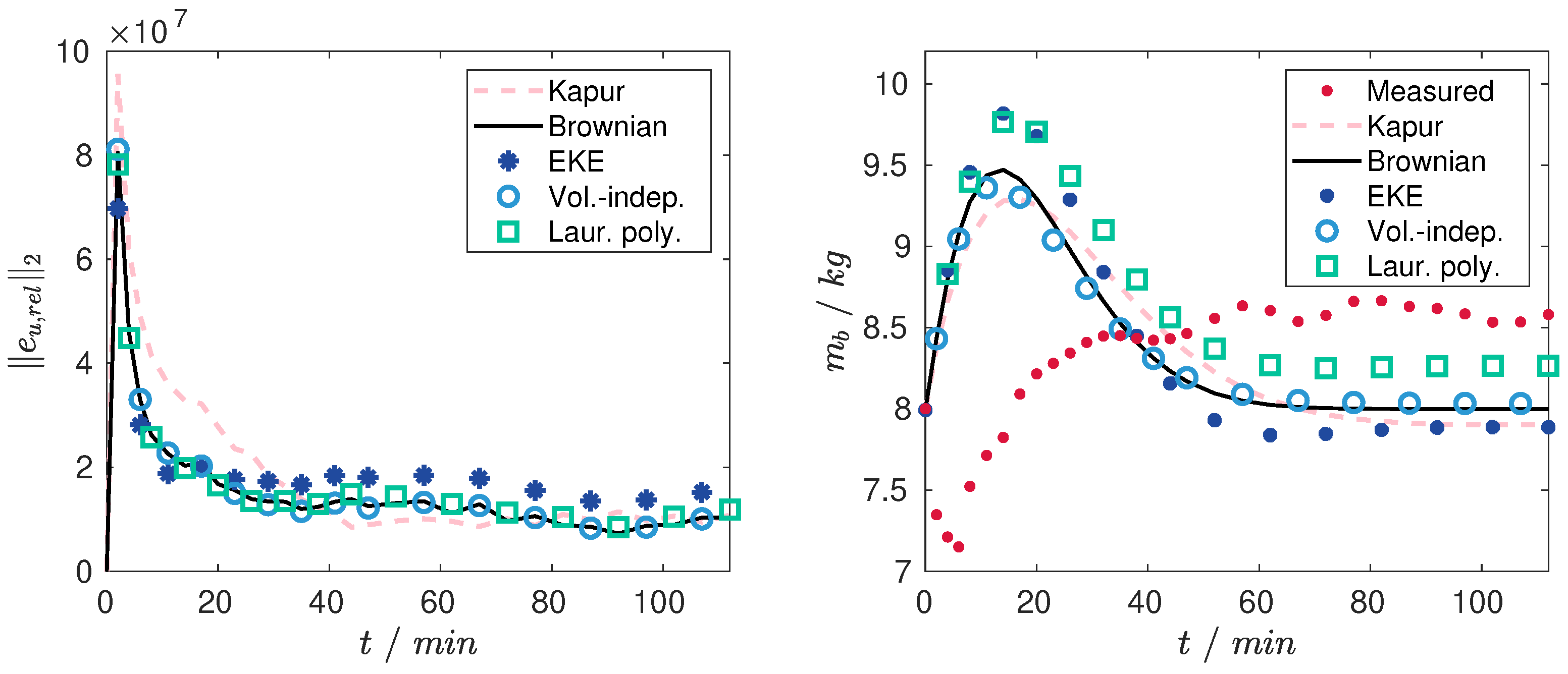
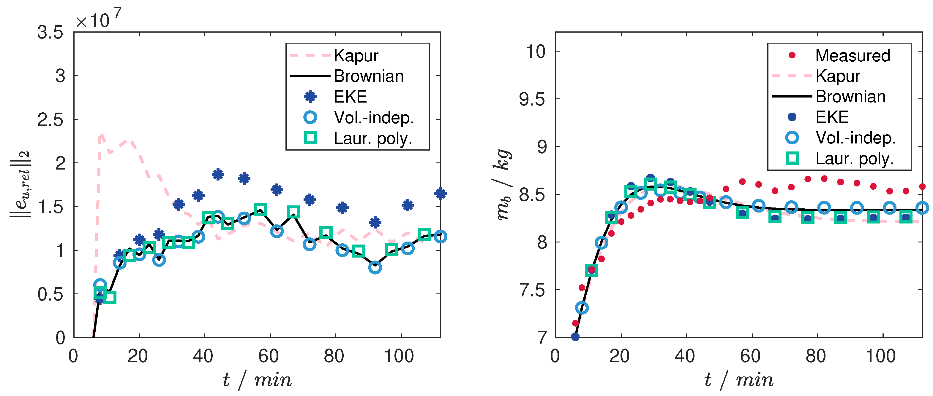
Applying the proposed approach for all five kernels and using the first experimental sample as initial condition yields in estimates for the agglomeration efficiency ${\beta }_0$ and the Laurent polynomials coefficients, respectively. The obtained results are depicted in Figure 3. As can be seen from the $L_2$-norm of the errors between measured and simulated PSD (Figure 3 (left)) and the simulated and measured bed mass (Figure 3 (right)), the mismatch for all fitted models is considerable in the first ten minutes of the process and decreases rapidly for larger process times. Here, the models with the Brownian motion kernel, the volume-independent kernel and the Laurent polynomials perform better, in terms of the $L_2$-norm, than the models with EKE and Kapur kernel.

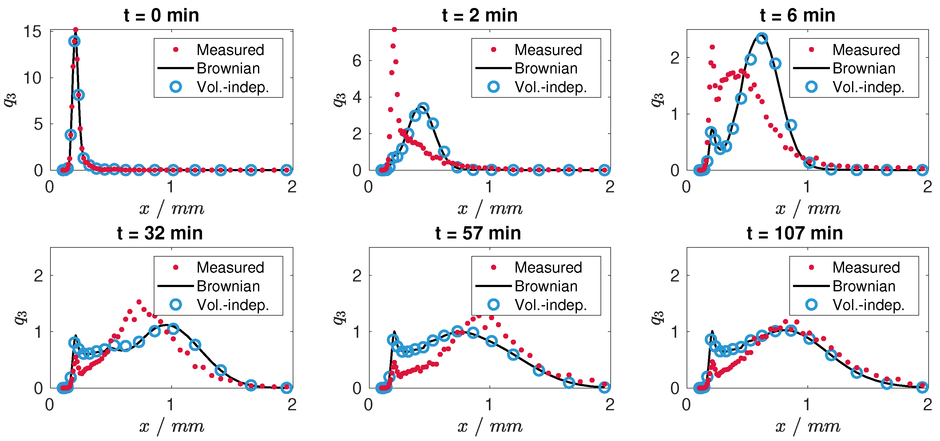
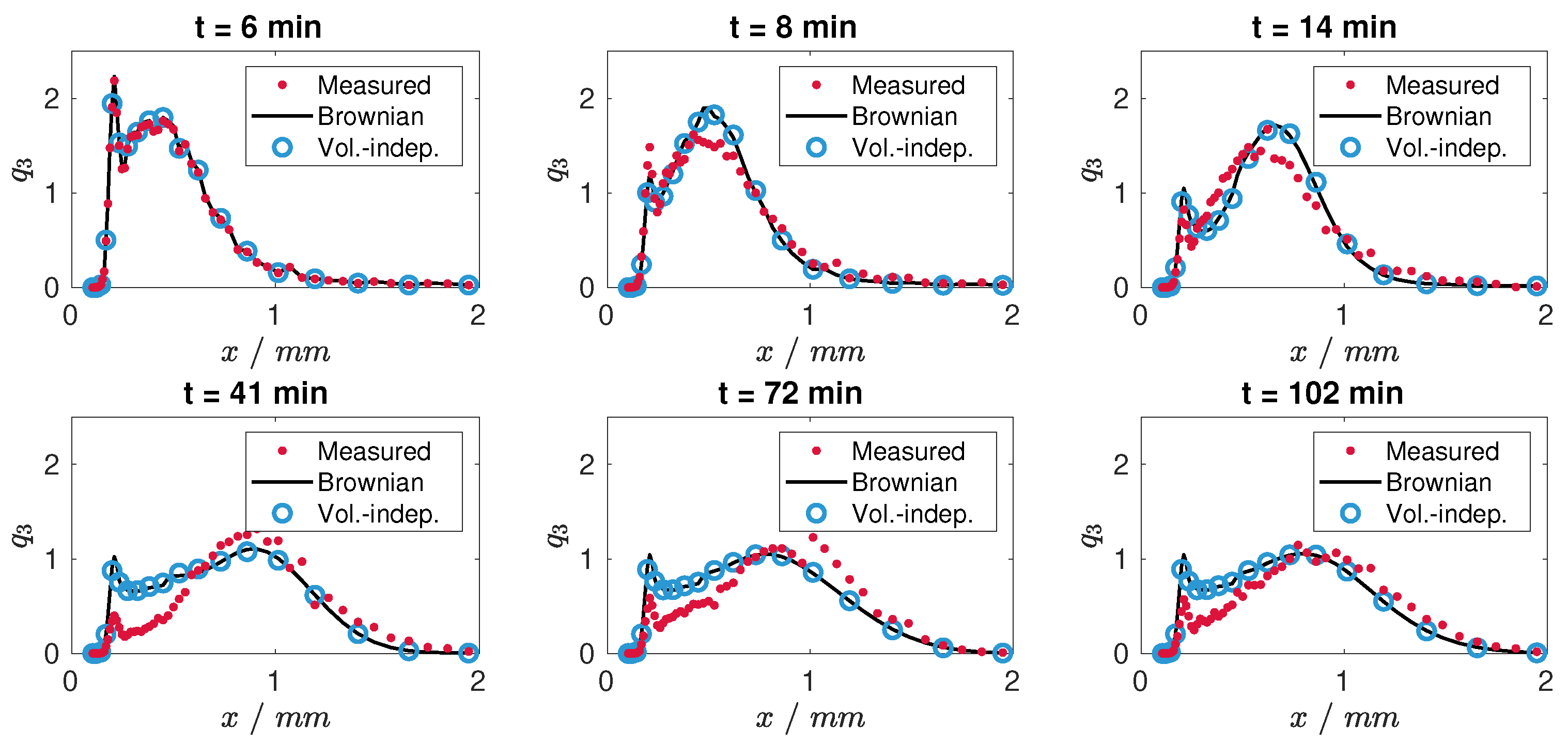
Figure 4 shows the comparison of the fitted models based on the Brownian motion and volume-independent kernels and the measured PSD in terms of normalized PSD $q_3(t,x)$

$$\begin{array}{c}\hfill q_3(t,x)=\frac{x^{3}n(t,x)}{{\int }_0^{\infty }{x}^{3}n(t,x)dx}\end{array}$$

(21)

For $t>80$ min no significant change in the normalized particle size distributions was obtained in the experiment, indicating steady-state operation.

Generally, it can be seen that the results improve for larger time values, i.e., closer to the steady-state operation. The big misfit in the initial phase demonstrates that the model structure does not reflect the start-up dynamics of the agglomeration process. Possible reasons may be additional internal transients, e.g., a temperature decrease due to spraying, which would result in a time-varying kernel. In addition, the decrease in the actual bed mass, which can be observed in the first couple of minutes, indicates that during start-up even particles being smaller than the product fraction are withdrawn from the process. This is however not reflected by the model, where a constant separation function for the product removal has been assumed. However, as the focus in this contribution and future research is on continuous agglomeration, only the dynamic behavior close to the steady-state is of importance. Therefore, in the following the initial start-up, i.e., the first six minutes, will be neglected resulting in a shifted time-domain.

3.1.2. Identification for the Shifted Time Domain

In the following, the described parameter estimation will be repeated for all kernels for the experimental data shifted by 6 min. Here, the experimental data sample at $t=6$ min will be used as the initial condition. Results of the nonlinear optimization are depicted in Figure 5 and Figure 6. As can be seen the matching between the parametrized model and the measurements has been improved considerably. The misfit in the region of the first mode (Figure 6) is presumable due to the measurement uncertainties. As before, the best results, in terms of the $L_2$-norm, are achieved for the model with the Brownian motion kernel, the volume-independent kernel and the Laurent polynomials. Yet, the latter does not show significant improvement despite its higher number of model parameters and will therefore be excluded from subsequent analysis.

3.2. Model Identifiability

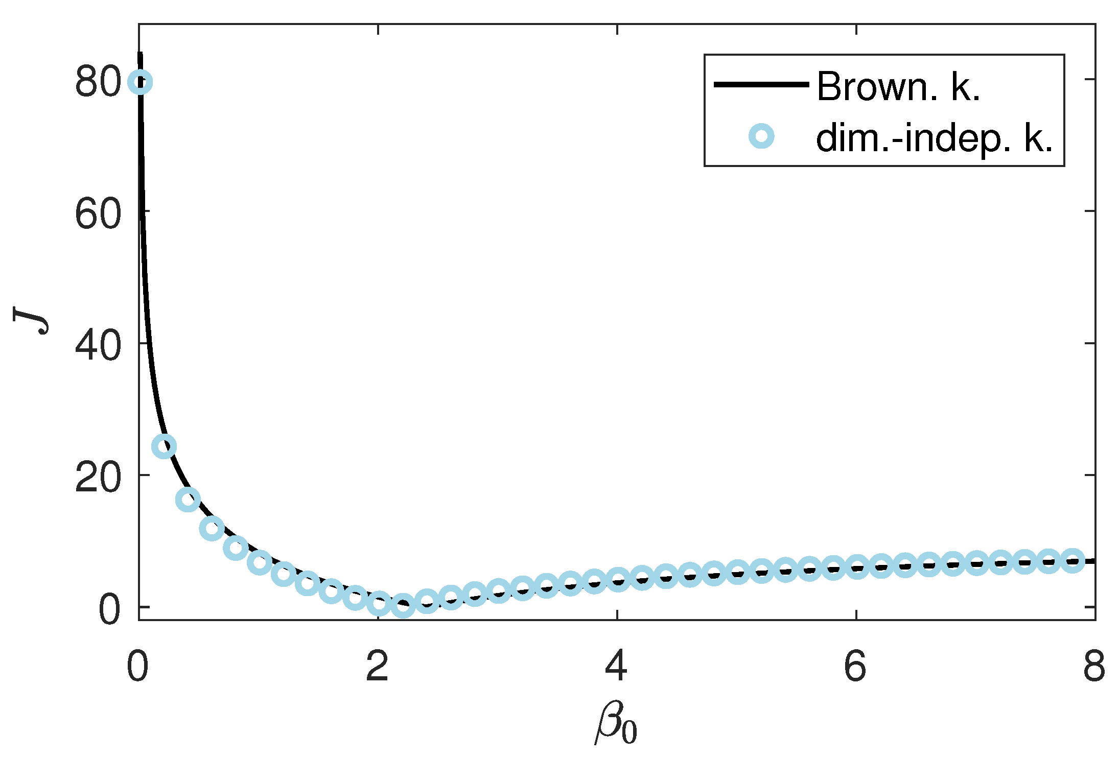
For the Brownian and volume-independent kernel, the agglomeration efficiency ${\beta }_0$ is the only unknown model parameter. Hence, the corresponding profile likelihood computation reduces to a parameter study, i.e., evaluation of the cost functional J for different values of ${\beta }_0$. The resulting curves, depicted in Figure 7, possess a distinct minimum, which indicates that the unknown ${\beta }_0$ is structurally identifiable in both cases.

3.3. Confidence Intervals

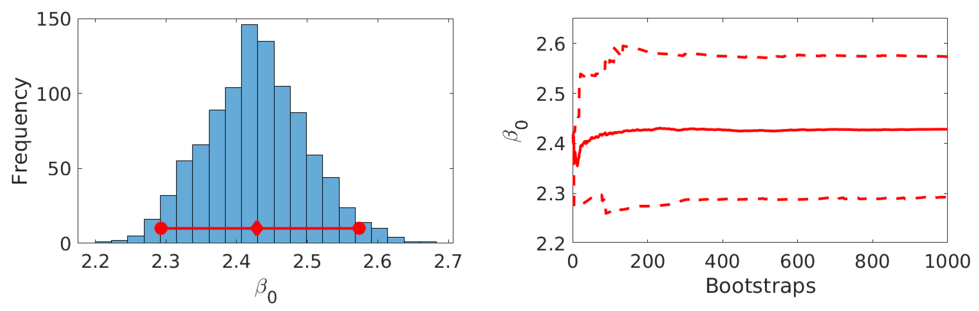
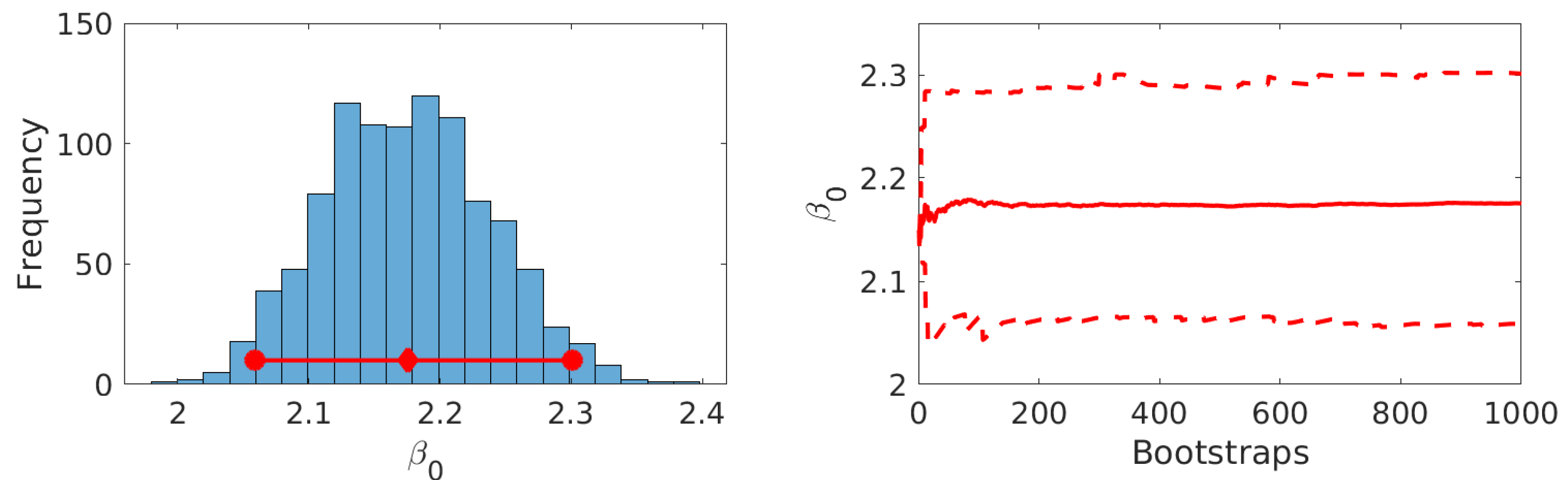
To compute parameter confidence intervals, a set of 1000 parametric bootstrap measurements was generated from the fitted model. Here, it was assumed that the measurements of $q_3(t,x)$ were corrupted by a relative error

$$\begin{array}{c}\hfill q_3{(t,x)}_k^{BS}=q_3{(t,x)}^{\ast }+q_3^{res}{(t,x)}_k^{BS},q_3^{res}{(t,x)}_k^{BS}\sim \mathcal{N}(0,{\Sigma }_{q_3})·q_3{(t,x)}^{\ast },k=1,\dots ,N_{BS}\end{array}$$

(22)

and thus the corresponding residual $q_3^{res}{(t,x)}_k^{BS}$ is proportional to the magnitude of $q_3{(t,x)}^{\ast }$. For the total bed mass measurement, bootstrap measurements were generated assuming an relative error

$$\begin{array}{c}\hfill m_{bed}{\left(t\right)}_k^{BS}=m_{bed}{\left(t\right)}^{\ast }+m_{bed}^{res}{\left(t\right)}_k^{BS},m_{bed}^{res}{\left(t\right)}_k^{BS}\sim \mathcal{N}(0,{\Sigma }_{m_{bed}}),k=1,\dots ,N_{BS}\end{array}$$

(23)

The model was refitted to the bootstrapped measurement set for the Brownian motion and the volume-independent kernel. Results by means of histograms of the obtained bootstrapped parameter sets and percentile plots over the number of bootstrap runs are shown in Figure 8 and Figure 9.

It can be seen that for both cases approximately symmetric Gaussian-like distributions are obtained. Furthermore, it is shown that the values for the percentiles and the mean do not significantly change for $k>400$ thereby indicating convergence of the bootstrapped parameter distribution. The overall confidence intervals and means are given in

Table 4. Mean parameter values and confidence intervals from parametric bootstrap.

Agglomeration Kernel	${\overline{\mathit{\beta }}}_0$	$\left[{\mathit{\beta }}_0^{\mathit{lo}},{\mathit{\beta }}_0^{\mathit{up}}\right]=\left[{\mathit{\beta }}_0^{0.025},{\mathit{\beta }}_0^{0.975}\right]$
Brownian motion	$2.4284\times {10}^{-11}$	$\left[2.2926\times {10}^{-11},2.5736\times {10}^{-11}\right]$
Volume-independent	$2.1754\times 5\times {10}^{-12}$	$\left[2.0588\times 5\times {10}^{-12},2.3011\times 5\times {10}^{-12}\right]$

.

4. Conclusions

In this paper the parameter identification for continuous fluidized bed spray agglomeration was presented. For the estimation of the agglomeration kernel from the experimental data a set of five different kernel model candidates has been fitted to experimental data applying nonlinear optimization. Applying the estimation procedure on the whole time domain showed that the initial start-up phase could not be reflected well by the given model structure. Possible reasons may be additional internal transients in this phase, e.g., temperature decrease due to spraying. Those would result in a time-varying kernel. However, the focus of future work is on the continuously operating agglomeration, process this initial phase is of minor importance. Therefore, the estimation procedure has been repeated for a shifted time domain, i.e., neglecting the first six minutes, resulting in significant better results. It has been shown that models based on the Brownian motion, the volume-independent and the Laurent polynomial kernel provide the best results in terms of the $L_2$-norm of the error based on the PSD. Despite its higher complexity and higher number of free model parameters, the latter approach is not superior to the two simpler kernel models. Thus, following good modelers practice, the Brownian and the volume-independent approaches were preferred. For both kernel models identifiability in terms of the corresponding profile likelihoods was shown and confidence intervals for the model parameters were determined using a parametric bootstrap method.

Future work will be concerned with qualitative process behavior for varying process conditions. As has been shown in earlier contributions, stability of continuously operated particulate processes strongly depends on the chosen process conditions (e.g., [32,33]). In order to increase robustness with respect to unforeseen disturbances and stabilize the process for varying operating conditions, feedback control will be studied. Here, a number of finite-dimensional [34,35] and infinite-dimensional [36] approaches have been investigated and developed for related continuous granulation processes in fluidized beds.

References

- Bück, A.; Tsotsas, E. Agglomeration. In Encyclopedia of Food and Health; Caballero, B., Finglas, P.M., Toldrá, F., Eds.; Academic Press: Oxford, UK, 2016; pp. 73–81. [Google Scholar] [CrossRef]
- Groenewold, H.; Tsotsas, E. Drying in fluidized beds with immersed heating elements. Chem. Eng. Sci. 2007, 62, 481–502. [Google Scholar] [CrossRef]
- Dadkhah, M.; Tsotsas, E. Influence of process variables on internal particle structure in spray fluidized bed agglomeration. Powder Technol. 2014, 258, 165–173. [Google Scholar] [CrossRef]
- Esmailpour, A.A.; Mostoufi, N.; Zarghami, R. Effect of temperature on fluidization of hydrophilic and hydrophobic nanoparticle agglomerates. Exp. Therm. Fluid Sci. 2018, 96, 63–74. [Google Scholar] [CrossRef]
- Zhao, H.; Maisels, A.; Matsoukas, T.; Zheng, C. Analysis of four Monte Carlo methods for the solution of population balances in dispersed systems. Powder Technol. 2007, 173, 38–50. [Google Scholar] [CrossRef]
- Terrazas-Velarde, K.; Peglow, M.; Tsotsas, E. Kinetics of fluidized bed spray agglomeration for compact and porous particles. Chem. Eng. Sci. 2011, 66, 1866–1878. [Google Scholar] [CrossRef]
- Rieck, C.; Schmidt, M.; Bück, A.; Tsotsas, E. Monte Carlo modeling of binder-Less spray agglomeration in fluidized beds. AIChE J. 2018, 64, 3582–3594. [Google Scholar] [CrossRef]
- Ramkrishna, D. Population Balances: Theory and Applications to Particulate Systems in Engineering; Academic Press: San Diego, CA, USA, 2000. [Google Scholar] [CrossRef]
- Cotabarren, I.; Schulz, P.G.; Bucalá, V.; Piña, J. Modeling of an industrial double-roll crusher of a urea granulation circuit. Powder Technol. 2008, 183, 224–230. [Google Scholar] [CrossRef]
- Cotabarren, I.M.; Bertín, D.E.; Bucalá, V.; Piña, J. Feedback control strategies for a continuous industrial fluidized-bed granulation process. Powder Technol. 2015, 283, 415–432. [Google Scholar] [CrossRef]
- Vreman, A.; van Lare, C.; Hounslow, M. A basic population balance model for fluid bed spray granulation. Chem. Eng. Sci. 2009, 64, 4389–4398. [Google Scholar] [CrossRef] [Green Version]
- Immanuel, C.D.; Doyle, F.J. Solution technique for a multi-dimensional population balance model describing granulation processes. Powder Technol. 2005, 156, 213–225. [Google Scholar] [CrossRef]
- Poon, J.M.H.; Immanuel, C.D.; Francis, J.; Doyle, I.; Litster, J.D. A three-dimensional population balance model of granulation with a mechanistic representation of the nucleation and aggregation phenomena. Chem. Eng. Sci. 2008, 63, 1315–1329. [Google Scholar] [CrossRef]
- Kumar, J.; Peglow, M.; Warnecke, G.; Heinrich, S.; Mörl, L. Improved accuracy and convergence of discretized population balance for aggregation: The cell average technique. Chem. Eng. Sci. 2006, 61, 3327–3342. [Google Scholar] [CrossRef]
- Bück, A.; Klaunick, G.; Kumar, J.; Peglow, M.; Tsotsas, E. Numerical Simulation of Particulate Processes for Control and Estimation by Spectral Methods. AIChE J. 2012, 58, 2309–2319. [Google Scholar] [CrossRef]
- Hussain, M.; Kumar, J.; Peglow, M.; Tsotsas, E. Modeling spray fluidized bed aggregation kinetics on the basis of Monte-Carlo simulation results. Chem. Eng. Sci. 2013, 101, 35–45. [Google Scholar] [CrossRef]
- Hussain, M.; Peglow, M.; Tsotsas, E.; Kumar, J. Modeling of aggregation kernel using Monte Carlo simulations of spray fluidized bed agglomeration. AIChE J. 2014, 60, 855–868. [Google Scholar] [CrossRef]
- Peglow, M.; Kumar, J.; Heinrich, S.; Warnecke, G.; Tsotsas, E.; Mörl, L.; Wolf, B. A generic population balance model for simultaneous agglomeration and drying in fluidized beds. Chem. Eng. Sci. 2007, 62, 513–532. [Google Scholar] [CrossRef]
- Aldous, D.J. Deterministic and Stochastic Models for Coalescence (Aggregation and Coagulation): A Review of the Mean-Field Theory for Probabilists. Bernoulli 1999, 5, 3–48. [Google Scholar] [CrossRef]
- Bramley, A.S.; Hounslow, M.J.; Ryall, R.L. Aggregation during Precipitation from Solution: A Method for Extracting Rates from Experimental Data. J. Colloid Interface Sci. 1996, 183, 155–165. [Google Scholar] [CrossRef]
- Mahoney, A.W. Inverse Problem Modeling of Particulate Systems. Ph.D. Thesis, Purdue University Graduate School, West Lafayette, IN, USA, 2001. [Google Scholar]
- Chakraborty, J.; Kumar, J.; Singh, M.; Mahoney, A.; Ramkrishna, D. Inverse Problems in Population Balances. Determination of Aggregation Kernel by Weighted Residuals. Ind. Eng. Chem. Res. 2015, 54, 10530–10538. [Google Scholar] [CrossRef]
- Eisenschmidt, H.; Soumaya, M.; Bajcinca, N.; Le Borne, S.; Sundmacher, K. Estimation of aggregation kernels based on Laurent polynomial approximation. Comput. Chem. Eng. 2017, 103, 210–217. [Google Scholar] [CrossRef]
- Vilas, C.; Arias-Méndez, A.; García, M.R.; Alonso, A.A.; Balsa-Canto, E. Toward predictive food process models: A protocol for parameter estimation. Criti. Rev. Food Sci. Nutr. 2018, 58, 436–449. [Google Scholar] [CrossRef] [PubMed]
- Van Hauwwermeiren, D.; De Beer, T.; Nopens, I. On the identifiability of kernels for population balance modelling. In Proceedings of the 6th International Conference on Population Balance Modelling, Gent, Belgium, 7–9 May 2018. [Google Scholar]
- Chis, O.T.; Banga, J.R.; Balsa-Canto, E. Structural Identifiability of Systems Biology Models: A Critical Comparison of Methods. PLoS ONE 2011, 6, e27755. [Google Scholar] [CrossRef] [PubMed] [Green Version]
- Raue, A.; Becker, V.; Klingmüller, U.; Timmer, J. Identifiability and observability analysis for experimental design in nonlinear dynamical models. Chaos 2010, 20, 045105. [Google Scholar] [CrossRef] [PubMed]
- Joshi, M.; Seidel-Morgenstern, A.; Kremling, A. Exploiting the bootstrap method for quantifying parameter confidence intervals in dynamical systems. Metab. Eng. 2006, 8, 447–455. [Google Scholar] [CrossRef] [PubMed]
- Joshi, M.; Kremling, A.; Seidel-Morgenstern, A. Model based statistical analysis of adsorption equilibrium data. Chem. Eng. Sci. 2006, 61, 7805–7818. [Google Scholar] [CrossRef]
- Schenkendorf, R.; Kremling, A.; Mangold, M. Optimal experimental design with the sigma point method. IET Syst. Biol. 2009, 3, 10–23. [Google Scholar] [CrossRef] [PubMed]
- Le Borne, S.; Shahmuradyan, L.; Sundmacher, K. Fast evaluation of univariate aggregation integrals on equidistant grids. Comput. Chem. Eng. 2015, 74, 115–127. [Google Scholar] [CrossRef]
- Dreyschultze, C.; Neugebauer, C.; Palis, S.; Bück, A.; Tsotsas, E.; Stefan, H.; Kienle, A. Influence of zone formation on stability of continuous fluidized bed layering granulation with external product classification. Particuology 2015, 23, 1–7. [Google Scholar] [CrossRef]
- Neugebauer, C.; Palis, S.; Bück, A.; Tsotsas, E.; Stefan, H.; Kienle, A. A dynamic two-zone model of continuous fluidized bed layering granulation with internal product classification. Particuology 2017, 31, 8–14. [Google Scholar] [CrossRef]
- Palis, S.; Kienle, A. Stabilization of continuous fluidized bed spray granulation with external product classification. Chem. Eng. Sci. 2012, 70, 200–209. [Google Scholar] [CrossRef]
- Palis, S.; Kienle, A. H∞ loop shaping control for continuous fluidized bed spray granulation with internal product classification. Ind. Eng. Chem. Res. 2013, 52, 408–420. [Google Scholar] [CrossRef]
- Palis, S.; Kienle, A. Discrepancy based control of particulate processes. J. Process Control 2014, 24, 33–46. [Google Scholar] [CrossRef]
Figure 1.
(Left) Real pilot scale fluidized bed used for experiments (Right) Schematic representation of fluidized bed spray agglomeration process.
Figure 2.
(Left) Scanning electron microscope (SEM) picture of primary particles; (Right) SEM picture of agglomerates at steady state.
Figure 3.
(Left) Comparisonof the norms of the particle size distribution (PSD) error for different kernel candidates (Right) Comparison of the actual bed mass and bed masses of the identified models.
Figure 4.
Snapshots of particle size distributions of the actual plant and identified models.
Figure 5.
Comparison of the norms of the PSD error (Left) and the actual bed mass and bed masses of the identified models (Right) for the shifted time domain.
Figure 6.
Particle size distributions of the actual plant and the identified models for the shifted time domain.
Figure 7.
Profile likelihoods for the Brownian motion and volume-independent kernel.
Figure 8.
Results for parameter estimation for Brownian motion kernel with parametric bootstrap data: Histogram of bootstrapped parameter set, confidence interval (red circles) and mean (red rectangle) (Left) Change of (dashed) and (solid) over number of bootstrap runs (Right).
Figure 9.
Results for parameter estimation for volume-independent agglomeration kernel with parametric bootstrap data: Histogram of bootstrapped parameter set, confidence interval (red circles) and mean (red rectangle) (Left) Change of (dashed) and (solid) over number of bootstrap runs (Right).