Toward a Comprehensive and Efficient Robust Optimization Framework for (Bio)chemical Processes

Abstract

Model-based design principles have received considerable attention in biotechnology and the chemical industry over the last two decades. However, parameter uncertainties of first-principle models are critical in model-based design and have led to the development of robustification concepts. Various strategies have been introduced to solve the robust optimization problem. Most approaches suffer from either unreasonable computational expense or low approximation accuracy. Moreover, they are not rigorous and do not consider robust optimization problems where parameter correlation and equality constraints exist. In this work, we propose a highly efficient framework for solving robust optimization problems with the so-called point estimation method (PEM). The PEM has a fair trade-off between computational expense and approximation accuracy and can be easily extended to problems of parameter correlations. From a statistical point of view, moment-based methods are used to approximate robust inequality and equality constraints for a robust process design. We also apply a global sensitivity analysis to further simplify robust optimization problems with a large number of uncertain parameters. We demonstrate the performance of the proposed framework with two case studies: (1) designing a heating/cooling profile for the essential part of a continuous production process; and (2) optimizing the feeding profile for a fed-batch reactor of the penicillin fermentation process. According to the derived results, the proposed framework of robust process design addresses uncertainties adequately and scales well with the number of uncertain parameters. Thus, the described robustification concept should be an ideal candidate for more complex (bio)chemical problems in model-based design.

1. Introduction

Intensive competition in the (bio)chemical industry increases the requirements for better process performance. Thus, model-based tools are frequently applied to design (bio)chemical processes optimally, i.e., to optimize their performance while satisfying relevant system constraints [1,2]. However, external disturbances and process uncertainties might affect the performance of the plants, which then would deviate from the expected and simulated process characteristics or even result in operation failures [3]. The reliability of the designed processes under various conditions and disturbances is called robustness. Optimization problems that account for process performance and robustness must be tackled to provide solutions for real plants of industrial relevance.

The concept of robust optimization (RO) was first proposed by [4] and has been extensively applied to design upstream synthesis units [5,6] and downstream separation units [3,7] for bio(chemical) processes. RO concepts can be categorized into three groups: worst-case [7,8], probability-based [5,6,9] and possibility-based [10]. The worst-case and possibility-based approaches are a good choice for crude uncertainty expressions, but might lead to conservative results [11]. Probability-based concepts, which include detailed parameter uncertainty information regarding probability density functions (PDFs), are very relevant and have attracted considerable attention in the last decade [5,6,11]. However, the probability-based RO requires methods for uncertainty propagation and quantification (UQ), which pose obvious challenges in computational efficiency and approximation accuracy. Thus, the credibility and flexibility of the RO approach are determined by the underlying numerical UQ methods [4,12].

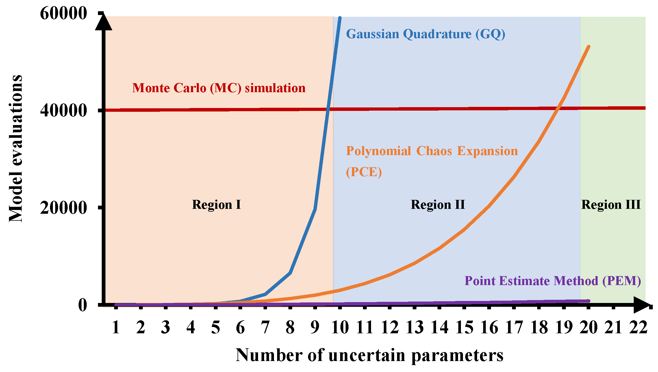
Various UQ methods for RO can be found in the literature. For instance, [13] used traditional sampling-based methods, i.e., (quasi) Monte Carlo (MC) simulation. Spectral methods, e.g., polynomial chaos expansion [14,15], have also been extensively used for RO [16,17,18], because of their fast convergence. Moreover, the desired statistical information can be calculated analytically. Gaussian quadrature (GQ), which was developed for solving numerical integration problems [19], is also a common approach for RO. These methods all have specific merits, but fall short in an essential aspect: they all suffer from the deficiency of computational expense. In this work, we propose the point estimate method (PEM) [2] for probability-based RO, because the PEM has superior efficiency compared to other UQ methods, as illustrated in Figure 1, and provides workable accuracy against various cubature methods, as concluded by [20,21]. Here, the computational demand (i.e., number of model evaluations) for different uncertainty quantification methods with the increasing number of uncertain parameters is illustrated to achieve similar approximation accuracy. The number of model evaluations for each method is determined based on the literature [15,20,22].

The dependencies of parameter uncertainties, which is referred to as parameter dependencies in the following context, commonly exist in practical applications [23,24,25], but are generally not taken into account in RO studies. Recently, this issue has received more attention in the field of sensitivity analysis [25,26,27], where parameter correlation has a significant impact on parameter sensitivities and the resulting probability distributions of the model output [20,28]. Therefore, in this work, we adapted the PEM by implementing an isoprobabilistic transformation step [29] to include parameters dependencies properly. Thus, the effect of parameter dependencies on the RO result is investigated and critically compared with the reference case where parameter dependencies are neglected.

This paper also provides a holistic framework for probability-based RO with the PEM. The objective function is robustified by using its first and second statistical moments. The multi-objective optimization problem is transferred to a single-objective optimization problem by taking the weighted sum of these moments [5]. Moreover, we distinguish between hard and soft constraints where only the latter case needs to be robustified. Soft equality constraints might also be relevant in the design of (bio)chemical processes, but were rarely considered in previous RO studies [30,31]. In this work, we provide a robust formulation for soft inequality and equality constraints and investigate their effect on the objective function. With the statistical moments estimated by the PEM, the second and fourth moment methods introduced by [32] for structural reliability analysis are implemented to approximate the robustified soft constraints. The fourth moment method has a more rigorous structure than the second moment method, but requires knowledge about the third and fourth statistical moments, which might be challenging for the PEM, as the approximation accuracy degrades for higher order statistical moments. Therefore, we demonstrate and compare the performance of the two methods for approximating the robust soft inequality constraints. Additionally, the global sensitivity analysis technique [22] is utilized to obtain a better understanding of the process under study and provide information for simplifying and constructing the robust optimization problem systematically.

The paper is organized as follows. Section 2 refers to the basics of probability-based RO. The PEM and its extension to arbitrary and correlated parameters are described in Section 3. Section 4 provides details about robust inequality and equality constraints and approximation methods. The final structure of probability-based RO is given in Section 5. The basics of the global sensitivity analysis are given in Section 6. To demonstrate the performance of the proposed RO framework, two case studies are thoroughly discussed in Section 7: including a classic jacket tubular reactor and a fed-batch bioreactor for penicillin fermentation. Conclusions can be found in Section 8.

2. Background of Probability-Based Robust Optimization

This section starts with the problem formulation used throughout the paper and introduces the general structure of probability-based RO. First-principle models are used to describe physicochemical mechanisms of (bio)chemical processes mathematically. In the field of process system engineering, mathematical models typically consist of nonlinear different algebraic equations (DAEs) equal to:

$$\begin{array}{ccc}\hfill {\dot{\mathbf{x}}}_{\mathbf{d}}(t)& ={\mathbf{g}}_{\mathbf{d}}(\mathbf{x}(t),\mathbf{u}(t),\mathbf{p}),& {\mathbf{x}}_{\mathbf{d}}(0)={\mathbf{x}}_0,\hfill \end{array}$$

(1)

$$\begin{array}{ccc}\hfill \mathbf{0}& ={\mathbf{g}}_{\mathbf{a}}(\mathbf{x}(t),\mathbf{u}(t),\mathbf{p}),& \hfill \end{array}$$

(2)

where $t\in [0,t_f]$ denotes the time, $\mathbf{u}\in {\mathbb{R}}^{n_u}$ the control input vector and $\mathbf{p}\in {\mathbb{R}}^{n_p}$ the time-invariant parameter vector. $\mathbf{x}=[{\mathbf{x}}_{\mathbf{d}},{\mathbf{x}}_{\mathbf{a}}]\in {\mathbb{R}}^{n_x}$ is the state vector, while ${\mathbf{x}}_d\in {\mathbb{R}}^{n_{x_d}}$ and ${\mathbf{x}}_a\in {\mathbb{R}}^{n_{x_a}}$ are the differential and algebra states, respectively. ${\mathbf{x}}_0$ is the vector of the initial conditions for the differential states. Furthermore, two types of functions ${\mathbf{g}}_{\mathbf{d}}:{\mathbb{R}}^{(n_{x_d}+n_{x_a})\times n_u\times n_p}\to {\mathbb{R}}^{n_{x_d}}$ and ${\mathbf{g}}_{\mathbf{a}}:{\mathbb{R}}^{(n_{x_d}+n_{x_a})\times n_u\times n_p}\to {\mathbb{R}}^{n_{x_a}}$ are given, which denote the differential vector field and algebraic expressions of the process model.

Typically, the time-invariant parameters $\mathbf{p}$ and initial conditions ${\mathbf{x}}_0$ are not known exactly. Measurement and process noise give rise to uncertainties in model parameters, which are estimated through model fitting [2,23,33]. In addition, disturbances from the environment and the accuracy of the measurement devices result in uncertain initial conditions. As we intend to use random variables to describe the uncertainties in the parameters and the initial conditions, we define a probability space ($\mathsf{\Omega },\mathcal{F},P$) with the sample space $\mathsf{\Omega }$, $\sigma$-algebra $\mathcal{F}$, and the probability measure P. $\mathbf{\theta }=[\mathbf{p}(\omega )$, ${\mathbf{x}}_0(\omega )$] is the vector of random variables, which are functions of $\omega \in \mathsf{\Omega }$ on the probability space and associated with continuous PDFs $\mathbf{f}(\mathbf{\theta })=[f_1({\theta }_1),\dots ,f_{n_{\theta }}({\theta }_{n_{\theta }})]$ and correlation matrix $\Sigma$.

Parameter and initial condition uncertainties result in model-based prediction variations, i.e., the outcome of Equations (1) and (2) must be considered as random variables, as well. Therefore, nominal (i.e., ignoring given parameter variations) optimal control problems do not give reliable solutions for realistic processes as a single realization of the uncertain parameters is used [11]. To derive reliable solutions for almost all realizations of uncertain parameters, the following RO problem has to be solved.

Problem 1.

Probability-based robust optimization problem

$$\underset{\mathbf{x}(·),\mathbf{u}(·)}{min}\mathbf{E}[M({\mathbf{x}}_{t_f})]+\alpha \mathbf{Var}[M({\mathbf{x}}_{t_f})],$$

(3)

$$\begin{array}{cc}\hfill & subjectto:\end{array}$$

$$\begin{array}{c}{\dot{\mathbf{x}}}_{\mathbf{d}}(t)={\mathbf{g}}_{\mathbf{d}}(\mathbf{x}(t),\mathbf{u}(t),\mathbf{p}),\end{array}$$

(4)

$$\begin{array}{c}\mathbf{0}={\mathbf{g}}_{\mathbf{a}}(\mathbf{x}(t),\mathbf{u}(t),\mathbf{p}),\end{array}$$

(5)

$$\begin{array}{c}{\mathbf{x}}_{\mathbf{d}}(0)={\mathbf{x}}_0,\end{array}$$

(6)

$$\begin{array}{c}\mathbf{Pr}[{\mathbf{h}}_{\mathbf{nq}}(\mathbf{x}(t),\mathbf{u}(t),\mathbf{p})\ge 0]\le {\epsilon }_{nq},\end{array}$$

(7)

$$\begin{array}{c}\mathbf{Pr}[{\mathbf{h}}_{\mathbf{eq}}(\mathbf{x}(t),\mathbf{u}(t),\mathbf{p})\ne 0]\le {\epsilon }_{eq},\end{array}$$

(8)

$$\begin{array}{c}{\mathbf{u}}_{min}\le \mathbf{u}\le {\mathbf{u}}_{max}.\end{array}$$

(9)

Here, $\mathbf{E}[·]$ and $\mathbf{Var}[·]$ denote the mean and the variance of the cost function $M({\mathbf{x}}_{t_f})$, respectively, $\mathbf{Pr}[·]$ denotes the probability measure, $\alpha$ denotes a scalar weight factor, ${\epsilon }_{nq}$ and ${\epsilon }_{eq}$ are tolerance factors, [${\mathbf{u}}_{min}$,${\mathbf{u}}_{max}$] are the upper and lower boundaries for the control input vector and ${\mathbf{x}}_{t_f}$ is the state vector at the end of the time horizontal $t_f$. In detail, $M({\mathbf{x}}_{t_f})$ denotes a Mayer objective term that is used for nominal optimal control problems. Please note that certain reformulations can be made to consider optimal Lagrange control problems, as well. The two functions ${\mathbf{h}}_{\mathbf{nq}}:{\mathbb{R}}^{(n_{x_d}+n_{x_a})\times n_u\times n_p}\to {\mathbb{R}}^{n_{nq}}$ and ${\mathbf{h}}_{\mathbf{eq}}:{\mathbb{R}}^{(n_{x_d}+n_{x_a})\times n_u\times n_p}\to {\mathbb{R}}^{n_{eq}}$ are used to represent the inequality and equality constraints, which come from process restrictions, such as temperature limitations. Equations (4) and (5) are the model equations that are considered as equality constraints as discussed in Section 4.

Problem 1 expresses the general formulation of the RO problem regarding probabilistic uncertainties. Equation (3) gives the robust form of the objective function $M({\mathbf{x}}_{t_f})$, where $\mathbf{E}[M({\mathbf{x}}_{t_f})]$ and $\mathbf{Var}[M({\mathbf{x}}_{t_f})]$ represent the expected performance and the robustness of the objective function, respectively. The trade-off between the performance and the robustness is adjusted by the weight factor $\alpha$. Equations (7) and (8) give the robust form of the inequality and equality constraints, respectively. They ensure that the probability of all constraint violations is less than or equal to a certain tolerance factor that can be adjusted according to given specifications and safety rules. However, to solve Problem 1 practically, we have to address the following two aspects. First, the estimation of the probabilities of both constraint violations cannot be solved in closed form, and standard numerical methods might be computationally demanding. Thus, highly efficient approximation routines have to be applied to ensure representative results. Second, the robust equality constraints in Equation (8) are infeasible and render RO insolvable. These two aspects are discussed and addressed in the following section.

3. Point Estimate Method

The point estimate method is a sample-based and an efficient cubature rule for approximating n-dimensional integrals [34,35,36]. It is analogous to the concept of the so-called unscented transformation presented by [37], which describes the parameter uncertainty with some deterministic sample points and approximate the statistics of outputs with the corresponding model evaluations, but has different deterministic sample points, associated weights and higher accuracy [34]. The PEM has been successfully applied in the field of sensitivity analysis [38] and optimal experimental design [39,40,41] to quantify the influence of measurement imperfections on system identification. A brief introduction to the PEM is given in Section 3.1. The concept of extending the PEM to problems with arbitrary and correlated parameter uncertainties is presented in Section 3.2.

3.1. Basics of the Point Estimate Method

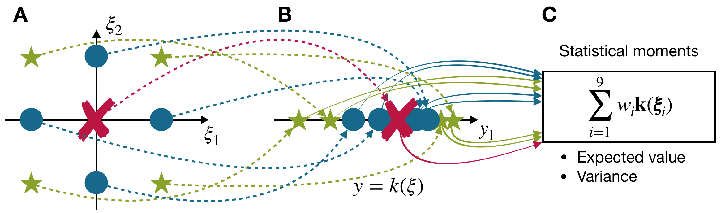
The basic principle of the PEM is illustrated in Figure 2. Here, a nonlinear function $\mathbf{k}(·)$ with a two-dimensional parameter $[{\xi }_1,{\xi }_2]$ and one model output $y_1$ is used for demonstration. We assume that the two parameters have a bivariate standard Gaussian distribution $\mathbf{\xi }\sim \mathcal{N}(\mathbf{0},\mathbf{I})$. The probability distribution of the parameters does not have to be Gaussian and could follow a uniform, beta distribution or any other parametric distribution; if it is symmetric and independent [41]. First, nine deterministic sample points, i.e., the cross, circle and star points in Figure 2, are generated and used for function evaluations. Finally, the integral term is approximated by a weighted superposition of these function evaluations equal to:

$${\int }_{{\mathbb{I}}_{\mathbf{\xi }}}\mathbf{k}(\mathbf{\xi })f(\mathbf{\xi })d\mathbf{\xi }\approx \sum _{i=1}^{n_p}{w}_i\mathbf{k}({\mathbf{\xi }}_i^s),$$

(10)

where ${\mathbf{\xi }}_i^s$ denotes the i-th sample point; $n_{\xi }$ and $n_p$ denote the number of random inputs and sample points, which are equal to two and nine in this example; $w_i$ is a scalar weight factor; and $f(\mathbf{\xi })$ is the PDF of the uncertain parameters.

The deterministic sample points used in this work are generated by the first three generator functions (GF[0], GF[$\pm \vartheta$], GF[$\pm \vartheta ,\pm \vartheta$]) defined in [34], which leads to an overall number of $n_p=2d^2+1$ sample points, where $d=n_{\xi }=n_{\theta }$. The specific weight factors are used for each generator function, which results in the final approximation scheme assuming standard Gaussian distributions:

$$\begin{array}{c}{\int }_{{\mathbb{I}}_{\mathbf{\xi }}}\mathbf{k}(\mathbf{\xi })f(\mathbf{\xi })d\mathbf{\xi }\approx \hfill \\ w_0\mathbf{k}(GF[0])+w_1\sum \mathbf{k}(GF[\pm \vartheta ])+w_2\sum \mathbf{k}(GF[\pm \vartheta ,\pm \vartheta ]),\hfill \end{array}$$

(11)

where $\vartheta =\sqrt{3},w_0=1+\frac{d^2-7d}{18},w_1=\frac{4-d}{18},w_2=\frac{1}{36}$ [38]. With these factors, Equation (11) provides suitable approximations for the integral of functions with moderate nonlinearities, i.e., system up to fifth-order [20,34]. Please note that the system with fifth-order means it can be accurately approximated with the sum of monomials up to order of five. In principle, we can also adapt the PEM to ensure lower or higher precision, but the proposed setting has the best trade-off between precision and computational costs [35].

3.2. Sampling Strategy for Independent/Correlated Random Variables of Arbitrary Distributions

As mentioned above, the proposed PEM is applicable only in the case of independent standard Gaussian distributions describing the parameter uncertainties. For most practical applications, however, we are confronted with problems of arbitrary and correlated probability distributions. Therefore, we extend the PEM by following Proposition 1.

Proposition 1.

For two random variables ($\mathbf{\theta },\mathbf{\xi }$), where $\mathbf{\xi }\sim \mathcal{N}(\mathbf{0},\mathbf{I})$ and θ has an arbitrary distribution and the function $\mathsf{\Phi }(·)=F_{\mathbf{\theta }}^{-1}(F_{\mathbf{\xi }}(·))$, the following relation for the integral terms of the nonlinear function $k(\mathbf{\theta })$ holds [20]:

$${\int }_{I_{\mathbf{\theta }}}k(\mathbf{\theta })f(\mathbf{\theta })d\mathbf{\theta }={\int }_{I_{\mathbf{\xi }}}k(\mathsf{\Phi }(\mathbf{\xi }))f(\mathbf{\xi })d\mathbf{\xi }.$$

(12)

Based on Proposition 1, the integral expression with an arbitrary correlation function is approximated as:

$${\int }_{{\mathbb{I}}_{\mathbf{\theta }}}\mathbf{k}(\mathbf{\theta })f(\mathbf{\theta })d\mathbf{\theta }\approx w_0\mathbf{k}(\mathsf{\Phi }({\mathbf{\xi }}^1))+w_1\sum _{i=2}^{2d+1}\mathbf{k}(\mathsf{\Phi }({\mathbf{\xi }}^i))+w_2\sum _{j=2d+2}^{2d^2+1}\mathbf{k}(\mathsf{\Phi }({\mathbf{\xi }}^j)),$$

(13)

where the samples from the original PEM for $\mathbf{\xi }$ are transformed via $\mathsf{\Phi }(·)=F_{\mathbf{\theta }}^{-1}(F_{\mathbf{\xi }}(·))$ to the corresponding points in $\mathbf{\theta }$, which can be directly evaluated with function $k(·)$. The joint cumulative density function (CDF) $F_{\mathbf{\theta }}(\mathbf{\theta })$ in $\mathsf{\Phi }(·)$ is typically unknown in practical applications and derived from marginal CDFs $[F_1({\theta }_1),\dots ,F_d({\theta }_d)]$ and the correlation matrix $\Sigma \in {\mathbb{R}}^{d\times d}$ for the uncertain parameter $\mathbf{\theta }$. Please note that it is actually infeasible to derive an analytical expression for $F_{\mathbf{\theta }}(\mathbf{\theta })$ and $\mathsf{\Phi }(·)$ [20]. Thus, we introduce Algorithm 1 to transform the samples from $\mathbf{\xi }$ to $\mathbf{\theta }$ numerically. The transformed sample points can be directly used for the approximation scheme:

$${\int }_{{\mathbb{I}}_{\mathbf{\theta }}}\mathbf{k}(\mathbf{\theta })f(\mathbf{\theta })d\mathbf{\theta }\approx w_0\mathbf{k}({\mathbf{\theta }}^1)+w_1\sum _{i=2}^{2d+1}\mathbf{k}({\mathbf{\theta }}^i)+w_2\sum _{j=2d+2}^{2d^2+1}\mathbf{k}({\mathbf{\theta }}^j).$$

(14)

Algorithm 1 is derived from the Nataf transformation procedure, which is based on Gaussian-copula [42]. By definition, the Gaussian-copula concept needs only the marginal distributions and the covariance matrix to approximate multivariate distributions. Technically, the Gaussian-copula is used for describing multivariate distributions with linear correlation, and thus might lose accuracy in describing multivariate distributions with non-linear correlations.

Algorithm 1 Sampling for correlated random variables

Initialization: Random variables $\mathbf{\xi }\sim \mathcal{N}(\mathbf{0},\mathbf{I})$, $I\in {\mathbb{R}}^{d\times d}$; $\mathbf{\theta }$ have marginal cumulative density functions $[F_1({\theta }_1),\dots ,F_d({\theta }_d)]$ and correlation matrix $\Sigma \in {\mathbb{R}}^{d\times d}$; 1: Sample $\mathbf{U}=[{\mathbf{\xi }}^1,\cdots ,{\mathbf{\xi }}^N]$ with size of $N=2d^2+1$ from $\mathbf{\xi }$ and dimension d from Generator function $GF[·]$; 2: Cholesky decomposition of $\Sigma =\mathbf{L}{\mathbf{L}}^T$, where L is a lower triangular matrix; 3: Correlate the sample, $\mathbf{V}=\mathbf{L}\mathbf{U}$; 4: Convert the sample to the corresponding cumulative density $\mathbf{W}={[F(V_1),\cdots ,F(V_d)]}^T$; 5: Transform into sample of $\mathbf{\theta }$, $[{\mathbf{\theta }}^1,\cdots ,{\mathbf{\theta }}^N]={[F_1^{-1}(W_1),\cdots ,F_d^{-1}(W_d)]}^T$.

4. Moment Method for Approximating Robust Inequality and Equality Constraints

In this section, we discuss the details of inequality and equality constraints. In Section 4.1, we categorize the constraints into two special types, i.e., hard and soft constraints, and discuss the effects of parameter uncertainties on the constraints. In Section 4.2 and Section 4.3, a robust formulation of soft inequality and soft equality constraints and methods for approximating the robustified expressions are presented.

4.1. Categorization of the Constraints

There are two types of robust inequality and equality constraints: hard and soft constraints [43]. Hard constraints must be satisfied regardless of uncertainties in the RO. Hard constraints ensure that optimized results satisfy physical laws. For instance, in Problem 1, equality constraints Equations (4) and (5), i.e., the governing equations, are hard constraints as they describe the underlying (bio)chemical processes and have to be consistently satisfied when assuming deterministic simulation results. Soft constraints, in turn, do not have to be exactly satisfied under uncertainties. Soft constraints (e.g., Equations (7) and (8)) are typically imposed by the designer to restrict the design space and to satisfy additional process specifications. Therefore, soft constraints can be satisfied only in a probabilistic manner and might occasionally be violated, i.e., an acceptable violation probability has to be defined for RO. Please note that the performance of the objective function may decrease if a very low violation probability is required. Soft constraints are considerably affected by parameter uncertainties and are investigated in the following section.

4.2. Robust Formulation of Soft Inequality Constraints

Soft inequality constraints do not have to be strictly satisfied, but in a probabilistic manner. Inequality constraints ${\mathbf{h}}_{\mathbf{nq}}(\mathbf{x}(t),\mathbf{u}(t),\mathbf{p})\le 0$ formulated on the probability space are also named chance constraints [44] and read as:

$$\mathbf{Pr}[{\mathbf{h}}_{\mathbf{nq}}(\mathbf{x}(t),\mathbf{u}(t),\mathbf{p})\le 0]\ge 1-{\epsilon }_{nq},$$

(15)

where the probability of constraint satisfaction must be higher or equal to $1-{\epsilon }_{nq}$. Please note that Equation (15) can also be equivalently transformed into Equation (16) when the probability of a constraint violation is used:

$$\mathbf{Pr}[{\mathbf{h}}_{\mathbf{nq}}(\mathbf{x}(t),\mathbf{u}(t),\mathbf{p})\ge 0]\le {\epsilon }_{nq}.$$

(16)

The probability of constraint violations is frequently estimated by MC simulations. A large number of samples are drawn from given parameter distributions, and the samples, where the constraints are violated, are counted. MC simulations are straightforward in implementation but require a considerable number of CPU-intensive model evaluations. The computational burden might be prohibitive, especially for the iterative nature of the RO. Moment-based approximation of failure probabilities has been widely applied in the field of reliability analysis [32], and thus, this method is used as an alternative concept to approximate the chance constraints in this work. In addition, it takes the advantage of the proposed PEM for estimating the needed statistical moments.

The basic idea of the moment-based approximation method is to transform the probability distribution of the constraint functions into some specific distributions, e.g., the standard normal distribution $\xi \sim \mathcal{N}(0,1)$ and to obtain the failure probability based on the probability. Here, the one-dimensional constraint function $-h_{nq}(\mathbf{x}(t),\mathbf{u}(t),\mathbf{p})$ with a negative sign is abbreviated as ${\overline{h}}_{nq}$ and used in the following. The isoprobabilistic transform given in Proposition 1 is applied to express the relation between the standard normal distribution and one random variable with given distribution as:

$$\xi =F_{\xi }^{-1}(F_{{\overline{h}}_{nq}}({\overline{h}}_{nq})),$$

(17)

where $F_{\xi }^{-1}$ indicates the inverse CDF of the standard normal distribution and $F_{{\overline{h}}_{nq}}$ indicates the CDF of $h_{nq}$. Based on this transformation, the failure probability of the constraint function ${\overline{h}}_{nq}$ is equivalent to the probability of $\xi \le F_{\xi }^{-1}(F_{{\overline{h}}_{nq}}(0))$ as shown in Equation (18). As the CDF of $\xi$ is known analytically, the failure probability of the constraint function can be determined if $F_{\xi }^{-1}(F_{{\overline{h}}_{nq}}(0))$ is given. However, the transformation function $F_{\xi }^{-1}(F_{{\overline{h}}_{nq}}(·))$ is typically not available as the CDF of ${\overline{h}}_{nq}$ is unknown in practice. Thus, we aim at transformation rules that are based only on the statistical moments of ${\overline{h}}_{nq}$ [32]:

$$\begin{array}{cc}\hfill \mathbf{Pr}[h_{nq}(\mathbf{x}(t),\mathbf{u}(t),\mathbf{p})\ge 0]& =\mathbf{Pr}[{\overline{h}}_{nq}\le 0],\hfill \\ \hfill & =\mathbf{Pr}[\xi \le F_{\xi }^{-1}(F_{{\overline{h}}_{nq}}(0))].\hfill \end{array}$$

(18)

Two representative moment-based approximation methods [32], i.e., the second moment method and the fourth moment method, are used to estimate the failure probability with the first four statistical moments of the probability distribution of the constraint function ${\overline{h}}_{nq}$, which are the mean (${\mu }_{{\overline{h}}_{nq}}$), variance (${\sigma }_{{\overline{h}}_{nq}}^2$), skewness (${\alpha }_{{\overline{h}}_{nq},3}$) and kurtosis (${\alpha }_{{\overline{h}}_{nq},4}$). The second moment method approximates the transformation function with the first two moments as in Equation (19), while the fourth moment method utilizes all four moments and has a more complex structure; see Equation (20) [32]. The approximations are incorporated in Equation (18) to calculate the failure probability of the constraints:

$$F_{\xi }^{-1}(F_{{\overline{h}}_{nq}}(0))=-\frac{{\mu }_{{\overline{h}}_{nq}}}{{\sigma }_{{\overline{h}}_{nq}}},$$

(19)

$$F_{\xi }^{-1}(F_{{\overline{h}}_{nq}}(0))=-\frac{3({\alpha }_{{\overline{h}}_{nq},4}-1)(\frac{{\mu }_{{\overline{h}}_{nq}}}{{\sigma }_{{\overline{h}}_{nq}}})+{\alpha }_{{\overline{h}}_{nq},3}({(\frac{{\mu }_{{\overline{h}}_{nq}}}{{\sigma }_{{\overline{h}}_{nq}}})}^2-1)}{\sqrt{(9{\alpha }_{{\overline{h}}_{nq},4}-5{\alpha }_{{\overline{h}}_{nq},3}^2-9)({\alpha }_{{\overline{h}}_{nq},4}-1)}}.$$

(20)

The accuracy of the moment-based approximation methods is determined by two factors. The first factor is the intrinsic approximation error, which results from the approximated transformation function (Equation (17)) using a limited number of statistical moments. By definition, the fourth moment method has a lower intrinsic approximation error because this method is more rigorously defined with higher order statistical moments. The second factor is the estimation error of the statistical moments, especially the higher order moments, e.g., skewness and kurtosis. The PEM introduced in Section 3 is used to calculate the needed statistical moments with considerably lower computational costs in comparison to MC simulations. However, the precision of the estimated statistical moments deteriorates with higher order statistical moments, because the PEM might fail for highly nonlinear problems of higher order terms. Thus, especially the fourth moment method may suffer from the estimation error. According to these two sources of approximation errors, it is difficult to determine which approximation method, i.e., the second or fourth moment method, is superior for robust process design. Therefore, we further analyze both concepts and investigate their benefits for efficient and credible robustification strategies in the following section.

4.3. Robust Formulation of soft Equality Constraints

Similar to the inequality constraints, soft equality constraints are considered in a probabilistic manner for the RO problem and are given as:

$$\mathbf{Pr}[{\mathbf{h}}_{\mathbf{eq}}(\mathbf{x}(t),\mathbf{u}(t),\mathbf{p})\ne 0]\le {\epsilon }_{eq}$$

(21)

However, Equation (21) is not directly solvable for most applications as the constraint function $h_{eq}$ has a continuous probability distribution. In other words, the probability of a single point is equal to zero when the random space is continuous [45]. Thus, we can find that:

$$\mathbf{Pr}[{\mathbf{h}}_{\mathbf{eq}}(\mathbf{x}(t),\mathbf{u}(t),\mathbf{p})\ne 0]=1,$$

(22)

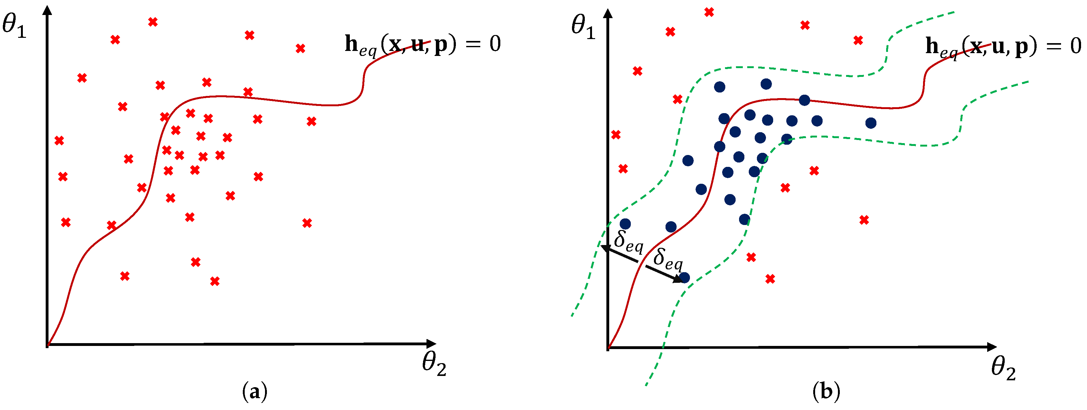
which contradicts Equation (21) if ${\epsilon }_{eq}⪇1$. Note that we aim to satisfy the equality constraint with high probability, and thus, ${\epsilon }_{eq}\ll 1$. Figure 3a shows an example of the equality constraint in the random parameter space. Here, the samples are drawn from their distributions, and the curve shows the locations where the samples satisfy the constraints.

To solve the RO problem, the robust equality constraints must be relaxed as shown in Figure 3b. This idea is analogous to the relaxed margin used in support vector machines (SVMs), which have been applied extensively in machine learning [46]. We ease the restriction from the constraints by admitting that samples can lie within a certain range around the constraints. Based on the relaxation, the robust equality constraints in Equation (21) are substituted by:

$$\mathbf{Pr}[-{\delta }_{eq}\le {\mathbf{h}}_{\mathbf{eq}}(\mathbf{x}(t),\mathbf{u}(t),\mathbf{p})\le {\delta }_{eq}]\ge 1-{\epsilon }_{eq},$$

(23)

where ${\delta }_{eq}$ indicates the relaxation factor and determines the range of relaxed equality constraints. As we can see in Figure 3b and Equation (23), we have a region rather than a single curve where the constraint is satisfied. Thus, we can have nonzero probability, and the RO problem becomes solvable. The robust equality constraints in Equation (23) have nearly the same structure as the robust inequality constraints in Equation (15). Therefore, the methods described in Section 4.2 can be used to solve Equation (23) in RO problems immediately.

As mentioned previously, there is a trade-off between the performance of the objective function and the satisfaction probability of soft inequality and soft equality constraints. The relevant factors, ${\epsilon }_{nq},{\epsilon }_{eq}$ and ${\delta }_{eq}$, have to be adapted properly. More details about how to select these factors are presented with the given case studies in Section 7.

5. Robust Optimization with the PEM

The final structure to solve the RO problem defined in Problem 1 is summarized in what follows. Note that $F(·)$ in Equations (31) and (32) indicates the CDF of a standard Gaussian distribution. The PEM is used to estimate the relevant statistical moments to include the effect of parameter uncertainties. Equations (26)–(30) are the evaluations of the dynamic system and the constraint functions for all deterministic sample points that are generated from the probability distributions of the uncertain model parameter. Based on the evaluations, Equations (34)–(39) calculate the statistical moments of the objective function and constraints, which are used in Equations (24), (31) and (32). Although Equations (31) and (32) demonstrate the approximation with the fourth moment method, we can easily switch to the second moment method by changing the structure from Equation (20) to Equation (19).

$$\begin{array}{c}\underset{\mathbf{x}(·),\mathbf{u}(·)}{min}\mathbf{E}[M({\mathbf{x}}_{t_f})]+\alpha \mathbf{Var}[M({\mathbf{x}}_{t_f})],\hfill \end{array}$$

(24)

$$\begin{array}{c}\mathrm{subject}\mathrm{to}:\hfill \end{array}$$

$$\begin{array}{c}i=1,\dots ,2d^2+1,m=1,2,3\hfill \end{array}$$

(25)

$$\begin{array}{c}{\mathbf{\theta }}_i={[{\mathbf{p}}_i,{\mathbf{x}}_{0,i}]}^T,{\mathbf{x}}_i={[{\mathbf{x}}_{\mathbf{d},i},{\mathbf{x}}_{\mathbf{a},i}]}^T,{\mathbf{x}}_{\mathbf{d},i}(0)={\mathbf{x}}_{0,i},{\mathbf{x}}_{t_f,i}={\mathbf{x}}_i(t_{final}),\hfill \end{array}$$

(26)

$$\begin{array}{c}{\dot{\mathbf{x}}}_{\mathbf{d},i}(t)={\mathbf{g}}_{\mathbf{d}}({\mathbf{x}}_i(t),\mathbf{u}(t),{\mathbf{p}}_i),\mathbf{0}={\mathbf{g}}_{\mathbf{a}}({\mathbf{x}}_i(t),\mathbf{u}(t),{\mathbf{p}}_i),\hfill \end{array}$$

(27)

$$\begin{array}{c}{\overline{h}}_{1,i}=-h_{nq}({\mathbf{x}}_i(t),\mathbf{u}(t),{\mathbf{p}}_i)\hfill \end{array}$$

(28)

$$\begin{array}{c}{\overline{h}}_{2,i}=h_{eq}({\mathbf{x}}_i(t),\mathbf{u}(t),{\mathbf{p}}_i)+{\delta }_{eq}\hfill \end{array}$$

(29)

$$\begin{array}{c}{\overline{h}}_{3,i}=-h_{eq}({\mathbf{x}}_i(t),\mathbf{u}(t),{\mathbf{p}}_i)+{\delta }_{eq}\hfill \end{array}$$

(30)

$$\begin{array}{c}F(-\frac{3({\alpha }_{{\overline{h}}_1,4}-1)(\frac{{\mu }_{{\overline{h}}_1}}{{\sigma }_{{\overline{h}}_1}})+{\alpha }_{{\overline{h}}_1,3}({(\frac{{\mu }_{{\overline{h}}_1}}{{\sigma }_{{\overline{h}}_1}})}^2-1)}{\sqrt{(9{\alpha }_{{\overline{h}}_1,4}-5{\alpha }_{{\overline{h}}_1,3}^2-9)({\alpha }_{{\overline{h}}_1,4}-1)}})\le {\epsilon }_{nq}\hfill \end{array}$$

(31)

$$\begin{array}{c}F(-\frac{3({\alpha }_{{\overline{h}}_2,4}-1)(\frac{{\mu }_{{\overline{h}}_2}}{{\sigma }_{{\overline{h}}_2}})+{\alpha }_{{\overline{h}}_2,3}({(\frac{{\mu }_{{\overline{h}}_2}}{{\sigma }_{{\overline{h}}_2}})}^2-1)}{\sqrt{(9{\alpha }_{{\overline{h}}_2,4}-5{\alpha }_{{\overline{h}}_2,3}^2-9)({\alpha }_{{\overline{h}}_2,4}-1)}})+F(-\frac{3({\alpha }_{{\overline{h}}_4,4}-1)(\frac{{\mu }_{{\overline{h}}_4}}{{\sigma }_{{\overline{h}}_4}})+{\alpha }_{{\overline{h}}_4,3}({(\frac{{\mu }_{{\overline{h}}_4}}{{\sigma }_{{\overline{h}}_4}})}^2-1)}{\sqrt{(9{\alpha }_{{\overline{h}}_4,4}-5{\alpha }_{{\overline{h}}_4,3}^2-9)({\alpha }_{{\overline{h}}_4,4}-1)}})\le {\epsilon }_{eq}\hfill \end{array}$$

(32)

$$\begin{array}{c}{\mathbf{u}}_{min}\le \mathbf{u}\le {\mathbf{u}}_{max},\hfill \end{array}$$

(33)

$$\begin{array}{c}\mathbf{E}[M({\mathbf{x}}_{t_f})]=w_{0}M({\mathbf{x}}_{t_f,1})+w_1\sum _{i=2}^{2d+1}M({\mathbf{x}}_{t_f,i})+w_2\sum _{j=2d+2}^{2d^2+1}M({\mathbf{x}}_{t_f,j}),\hfill \end{array}$$

(34)

$$\begin{array}{c}\hfill \begin{array}{c}\hfill \mathbf{Var}[M({\mathbf{x}}_{t_f})]=w_0{(M({\mathbf{x}}_{t_f,1})-\mathbf{E}[M({\mathbf{x}}_{t_f})])}^2+w_1\sum _{i=2}^{2d+1}{(M({\mathbf{x}}_{t_f,i})-\mathbf{E}[M({\mathbf{x}}_{t_f})])}^2\\ \hfill +w_2\sum _{j=2d+2}^{2d^2+1}{(M({\mathbf{x}}_{t_f,j})-\mathbf{E}[M({\mathbf{x}}_{t_f})])}^2,\end{array}\end{array}$$

(35)

$$\begin{array}{c}{\mu }_{{\overline{h}}_m}=w_0{\overline{h}}_{m,1}+w_1\sum _{i=2}^{2d+1}{\overline{h}}_{m,i}+w_2\sum _{j=2d+2}^{2d^2+1}{\overline{h}}_{m,j},\hfill \end{array}$$

(36)

$$\begin{array}{c}\hfill \begin{array}{c}\hfill {\sigma }_{{\overline{h}}_m}^2=w_0{({\overline{h}}_{m,1}-{\mu }_{{\overline{h}}_m})}^2+w_1\sum _{i=2}^{2d+1}{({\overline{h}}_{m,i}-{\mu }_{{\overline{h}}_m})}^2+\\ \hfill w_2\sum _{j=2d+2}^{2d^2+1}{({\overline{h}}_{m,j}-{\mu }_{{\overline{h}}_m})}^2,\end{array}\end{array}$$

(37)

$$\begin{array}{c}\hfill \begin{array}{c}\hfill {\alpha }_{{\overline{h}}_m,3}=\frac{w_0{({\overline{h}}_{m,1}-{\mu }_{{\overline{h}}_m})}^3+w_1{\displaystyle \sum _{i=2}^{2d+1}}{({\overline{h}}_{m,i}-{\mu }_{{\overline{h}}_m})}^3+w_2{\displaystyle \sum _{j=2d+2}^{2d^2+1}}{({\overline{h}}_{m,j}-{\mu }_{{\overline{h}}_m})}^3}{{\sigma }_{{\overline{h}}_m}^3},\end{array}\end{array}$$

(38)

$$\begin{array}{c}\hfill \begin{array}{c}\hfill {\alpha }_{{\overline{h}}_m,4}=\frac{w_0{({\overline{h}}_{m,1}-{\mu }_{{\overline{h}}_m})}^4+w_1{\displaystyle \sum _{i=2}^{2d+1}}{({\overline{h}}_{m,i}-{\mu }_{{\overline{h}}_m})}^4+w_2{\displaystyle \sum _{j=2d+2}^{2d^2+1}}{({\overline{h}}_{m,j}-{\mu }_{{\overline{h}}_{nq}})}^4}{{\sigma }_{{\overline{h}}_m}^4},\end{array}\end{array}$$

(39)

6. Global Sensitivity Analysis

Before we apply the robust optimization framework, we briefly introduce the idea of global sensitivity analysis (GSA). In general, GSA is not mandatory for the robust optimization framework but provides useful information for analyzing and optimizing complex systems.

GSA is a valuable tool for determining the impact of individual parameters and parameter combinations on the result of a mathematical model for given parameter variations [41,47,48,49,50,51]. Thus, GSA determines the most relevant parameters and parameter uncertainties to be considered in RO. By focusing on the relevant parameters and neglecting the insensitive parameters, we can reduce the complexity of the RO problem considerably.

As most model parameters, which are identified via experimental data, are correlated, the effect of parameter correlation has to be considered in GSA. In this work, we present GSA methods that are capable of problems with independent parameters and problems with dependent parameters. Although parameter dependence is quite common in practical applications, studies of GSA with dependent parameters have been considered only recently; see [25,26,27]. Moreover, the GSA concepts can be categorized into two types: variance-based methods [22,52,53] and moment-independent methods [54]. For details about the definitions and a critical comparison of these two concepts, the interested reader is referred to [55].

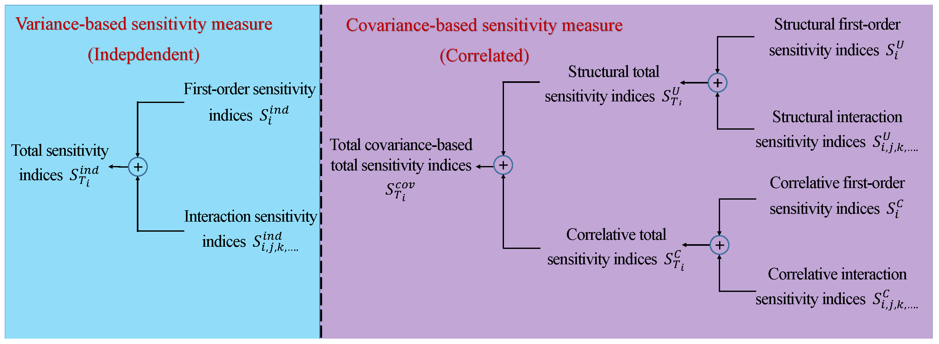
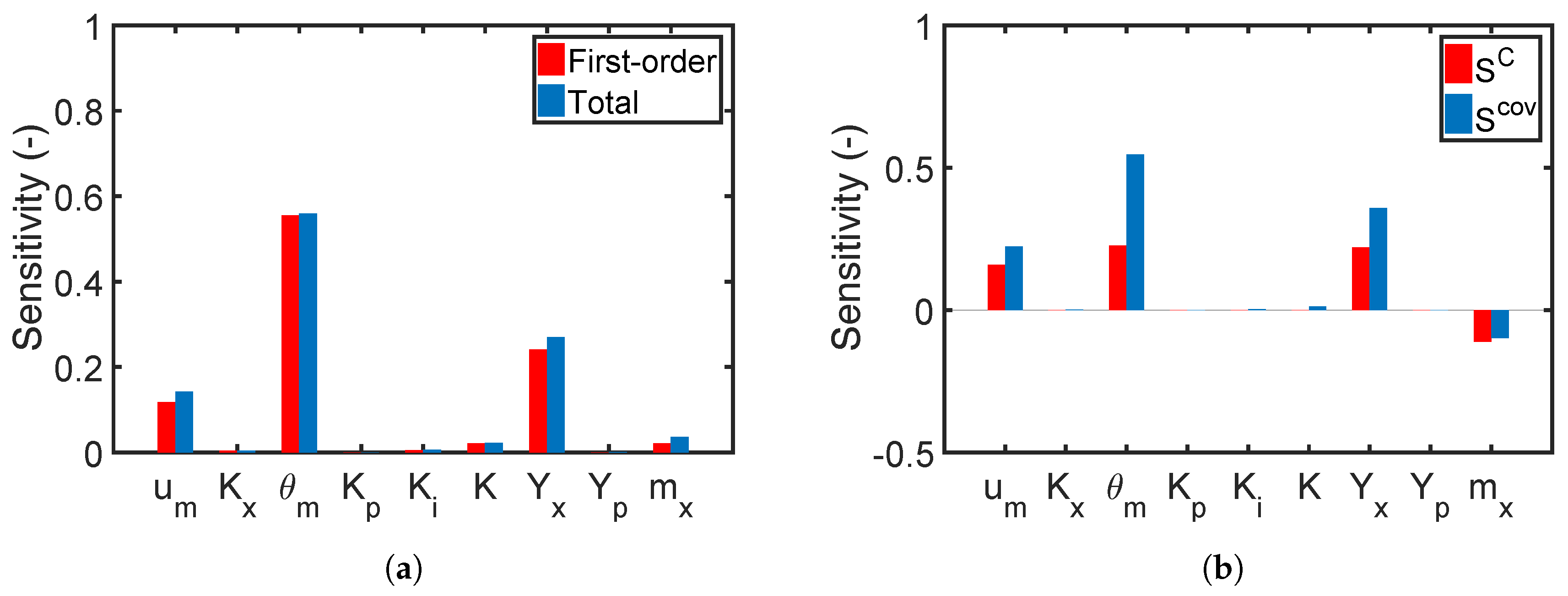
Although the moment-independent method has a more rigorous definition than the variance-based method, the variance-based approach is the standard in GSA, and thus, it is implemented in this work. The structure and types of sensitivity indices used in the variance-based method are illustrated in Figure 4. On the left of Figure 4, the variance-based method defines three types of sensitivity indices for independent parameters. First-order sensitivity indices $S_i^{ind}$ measure the main effect of an individual parameter i on the model output, interaction sensitivity indices $S_{i,j,k,\dots }^{ind}$ measure the dependence of the effect for two or more parameters, and total sensitivity indices $S_{T_i}^{ind}$ are the sum of the main and interactive effects of parameter i. On the right of Figure 4, new sensitivity indices are derived from the covariance decomposition of the model output for correlated parameters. They have the same types of sensitivity indices as the independent case but for three different groups: structural sensitivity indices $S^U$, correlative sensitivity indices $S^C$, and total covariance-based sensitivity indices $S^{cov}$. Structural sensitivity indices reflect the impact of an individual model parameter or parameter interactions on the model output and are determined by the model structure. They have the same trend as independent sensitivity indices but with different magnitudes. The correlative sensitivity indices exclusively show the impact of parameter correlations. The sum of these indices leads to total covariance-based sensitivity indices $S^{cov}$ that express the overall impact of the correlated parameters. In this work, the first-order sensitivity indices $S_i^{ind}$ for the independent case and the total covariance-based first-order sensitivity indices $S_i^{cov}$ for the correlated case are sufficient, because there are few interactions between the uncertain parameters. Values of the sensitivity indices were utilized as indicators for reducing the complexity of our RO problem as demonstrated in the design of the penicillin fermentation process.

7. Case Studies

In this section, we demonstrate the performance of the proposed framework with two case studies. In Case Study 1, we design an optimal jacket temperature profile for a tubular reactor considering two uncertain and correlated model parameters. Additionally, a robust equality constraint for the product temperature at the reactor outlet is assumed to incorporate process intensification aspects in the design problem. In Case Study 2, a penicillin fermentation process is analyzed as it is of interest in the pharmaceutical industry. A fed-batch bioreactor model is used to design an optimal feeding profile under parameter uncertainties. GSA is applied to determine the influence of parameter uncertainties on the process states and to offer a more tractable problem, i.e., a reduced number of uncertain model parameters, which have to be considered in the robust process design.

GSA and the RO problem were solved in MATLAB^® (Version 2017b, The MathWorks Inc., Natick, MA, USA). Parameter sensitivities for the independent case were calculated with UQLAB (Version 1.0, ETH Zurich, Switzerland) [56]. The RO problem for the first case study was solved with the MATLAB function fmincon, while the RO problem for the second case study, which is more complex, was solved by the simultaneous approach [57] and implemented in the symbolic framework CasADi (Verion 3.3.0, KU Leuven, Belgium) for numerical optimization [58] using the NLP solver IPOPT [59] and the MA57 linear solver [60].

7.1. Case Study 1: A Jacket Tubular Reactor

Here, the design of a tubular reactor, where an irreversible first-order reaction Equation (40) takes place, is considered the first benchmark case study.

$$A\stackrel{}{\to }B+C.$$

(40)

The reactor, which is operated under the steady-state condition, is described by the following governing Equations [31]:

$$\begin{array}{cc}\hfill \frac{d{\mathbf{x}}_1}{dz}& =\frac{{\alpha }_{kin}}{v}(1-{\mathbf{x}}_1)e^{\frac{\gamma {\mathbf{x}}_2}{1+{\mathbf{x}}_2}},\hfill \end{array}$$

(41)

$$\begin{array}{cc}\hfill \frac{d{\mathbf{x}}_2}{dz}& =\frac{{\alpha }_{kin}\delta }{v}(1-{\mathbf{x}}_1)e^{\frac{\gamma {\mathbf{x}}_2}{1+{\mathbf{x}}_2}}+\frac{\beta }{v}(\mathbf{u}-{\mathbf{x}}_2),\hfill \end{array}$$

(42)

where z is the relative position along the reactor, $0\le$ z $\le 1$. The states ${\mathbf{x}}_1$ and ${\mathbf{x}}_2$ are the dimensionless forms of the reactant concentration of A and the reactor temperature, respectively. The jacket temperature is the control input given in its dimensionless form $\mathbf{u}=(T_j-T_{in})/T_{in}$ and is adjusted to meet the desired performance and robustness requirements. The control input is discretized into 25 equidistant elements constrained by 280 K and 400 K. The kinetic coefficient ${\alpha }_{kin}$ and the heat transfer coefficient $\beta$ are assumed to be uncertain, i.e., they follow a Gaussian distribution with a standard deviation of 10% of their nominal values. The implemented parameter values and operating conditions are summarized in

Table 1. Parameters for the tubular reactor model.

Parameters	Unit	Nominal Value	Uncertainty
$x_1(0)$	-	0	-
$x_2(0)$	-	0	-
${\alpha }_{kin}$	s−1	0.058	$\mathcal{N}(0.058,{0.0058}^2)$
$\beta$	s−1	0.2	$\mathcal{N}(0.2,{0.02}^2)$
v	ms−1	0.1	-
$\gamma$	-	16.66	-
$\delta$	-	0.25	-

. For additional details of the proposed reactor model, the interested reader is referred to [31]. The conversion of the reactor $C_f$, as well as the reactor temperature $T_r$, can be calculated from their dimensionless form via:

$$\begin{array}{ccc}\hfill C_f(z=1)& =& x_1(z=1),\hfill \end{array}$$

(43)

$$\begin{array}{ccc}\hfill T_r(z)& =& x_2(z)\times T_{in}+T_{in}.\hfill \end{array}$$

(44)

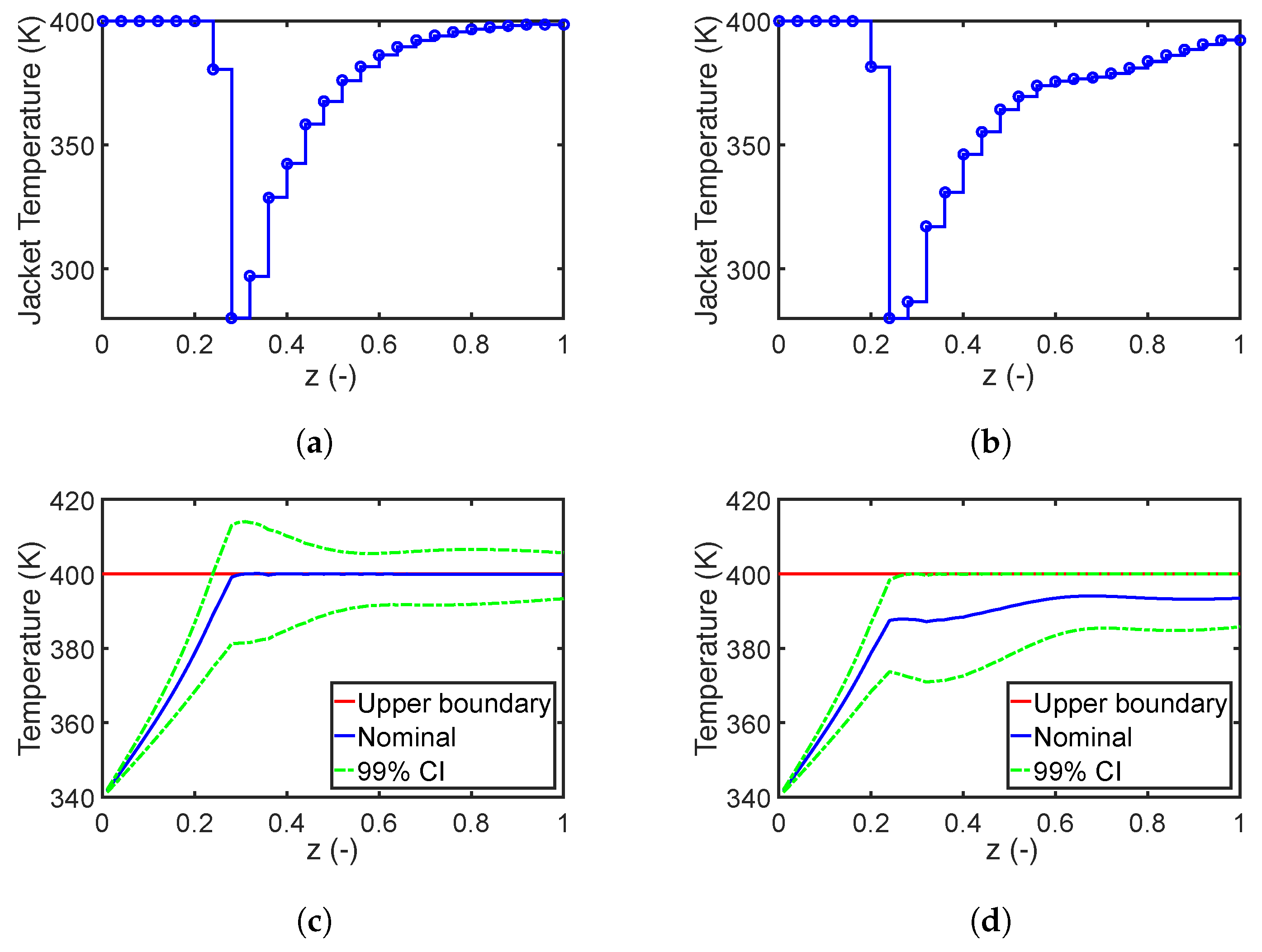
In this case study, we aim to maximize the final conversion of reactant A while fulfilling the given constraints on the reactor temperature. In particular, an upper boundary is added to the reactor temperature to prevent undesired side reactions. The results of the deterministic optimal design are depicted on the left of Figure 5. As we can see, the reactor temperature increases rapidly to the upper boundary to ensure the maximum reaction rate and final conversion of 0.996, respectively. However, numerous violations of the temperature boundary occur when the parameter uncertainties are taken into account. In contrast to the deterministic process design, a robust optimal design that includes parameter uncertainties is conducted next. Here, a weight factor $\alpha =3$ and a tolerance value ${\epsilon }_{nq}=1\%$ are used for the robust objective and inequality constraints. Please note that the weight factor $\alpha$ indicates the amount of trade-off between process performance and robustness of objective function, and is selected based on our previous studies [6]. The tolerance value ${\epsilon }_{np}=1\%$ means the robust solution has to guarantee that the violation probability of inequality constraints should not be larger than $1\%$, and could be changed depending on robustness required for the inequality constraint. The robust inequality constraints are approximated with the second moment method as in Equation (19). The corresponding results are given on the right of Figure 5. As we can see from the results, the jacket temperature profile is different from the nominal design, especially from location $0.3$ to the end of the reactor. Moreover, the reactor temperature profile of the robust design remains below its upper limit with a probability of 99% with the loss in the reactor performance; i.e., final conversion decreases to 0.985.

7.1.1. Robust Design with Parameter Correlation

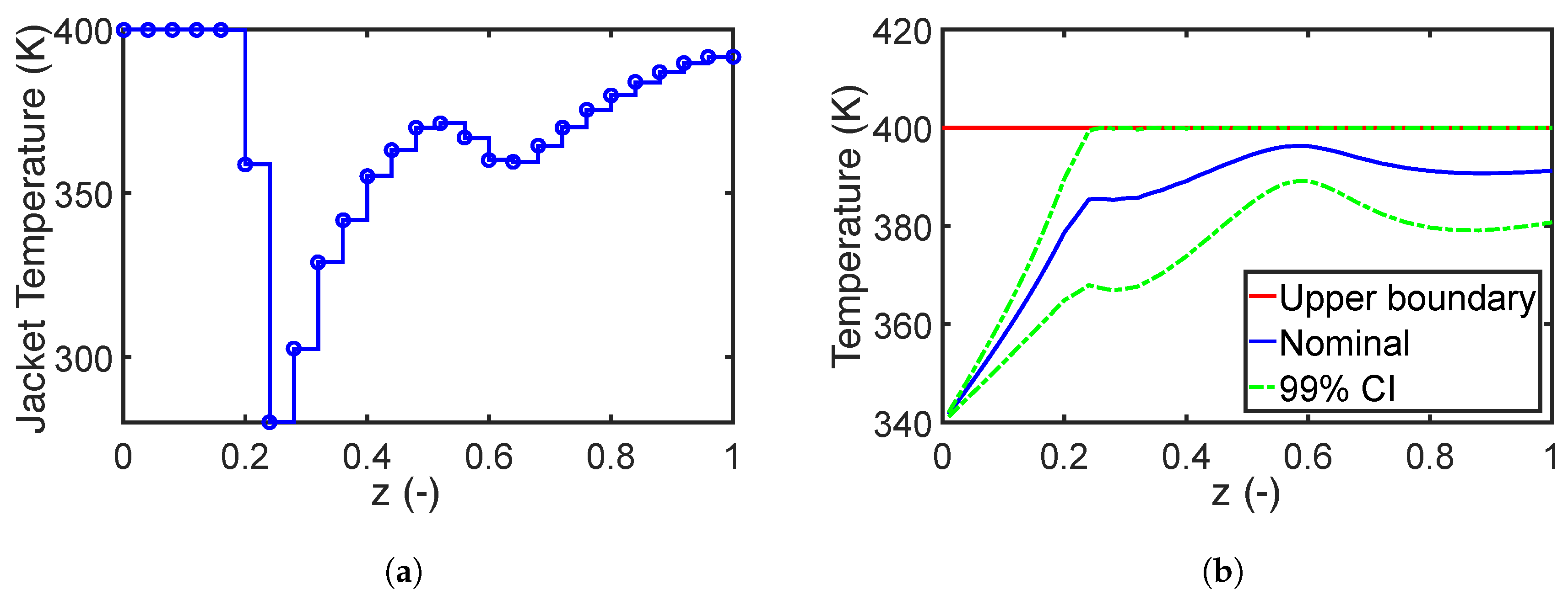
Next, we investigate the influence of parameter correlation on the robust process design. We assign the two uncertain parameters ${\alpha }_{kin}$ and $\beta$ with the marginal distributions shown in Table 1 and the additional Pearson correlation coefficient of 0.8. Deterministic sample points for the correlated parameters are generated with Algorithm 1 of the modified PEM. The structure of the RO problem is similar to that for independent parameters with a weight factor $\alpha =3$ and a tolerance value ${\epsilon }_{nq}=1\%$. Here, too, the second moment method is applied. In Figure 6, results for the optimal design with parameter correlation are given. As we can see, the profile of the jacket temperature has considerable differences compared to the nominal case; see Figure 5. Especially, the drop in the jacket temperature between position $z=0.5$ and $z=0.8$ results from the parameter correlation effect.

7.1.2. Performance of the Fourth Moment Method

Thus far, only the second moment method has been used to approximate the robust inequality constraints. The resulting confidence intervals of the reactor temperature are illustrated with green dashed curves in Figure 5d and Figure 6b. We can observe that the upper boundary of the confidence intervals are consistent with the upper limit of the reactor temperature once they approach it. However, the confidence intervals are approximated by taking into account only the first and second statistical moments and are insufficient if the probability distribution of the reactor temperature is non-Gaussian. Reference values based on MC simulations with 10,000 sample points are summarized in

Table 2. The number of constraint violations from 10,000 Monte Carlo simulations, where the robust inequality constraints are approximated by the second and fourth moment methods for process designs with independent and correlated parameters.

	Second Moment Method			Fourth Moment Method
Number of	Independent	Correlated			Independent	Correlated
violations	470	357			440	385
Probability	0.047	0.036			0.044	0.039

. In the case of the second moment method, the violation probabilities are 4.7% and 3.6%, respectively, which exceeds the tolerance value ${\epsilon }_{nq}=1\%$. The reason for this mismatch is mainly due to the approximation error of the robust inequality constraints while considering only the first two statistical moments.

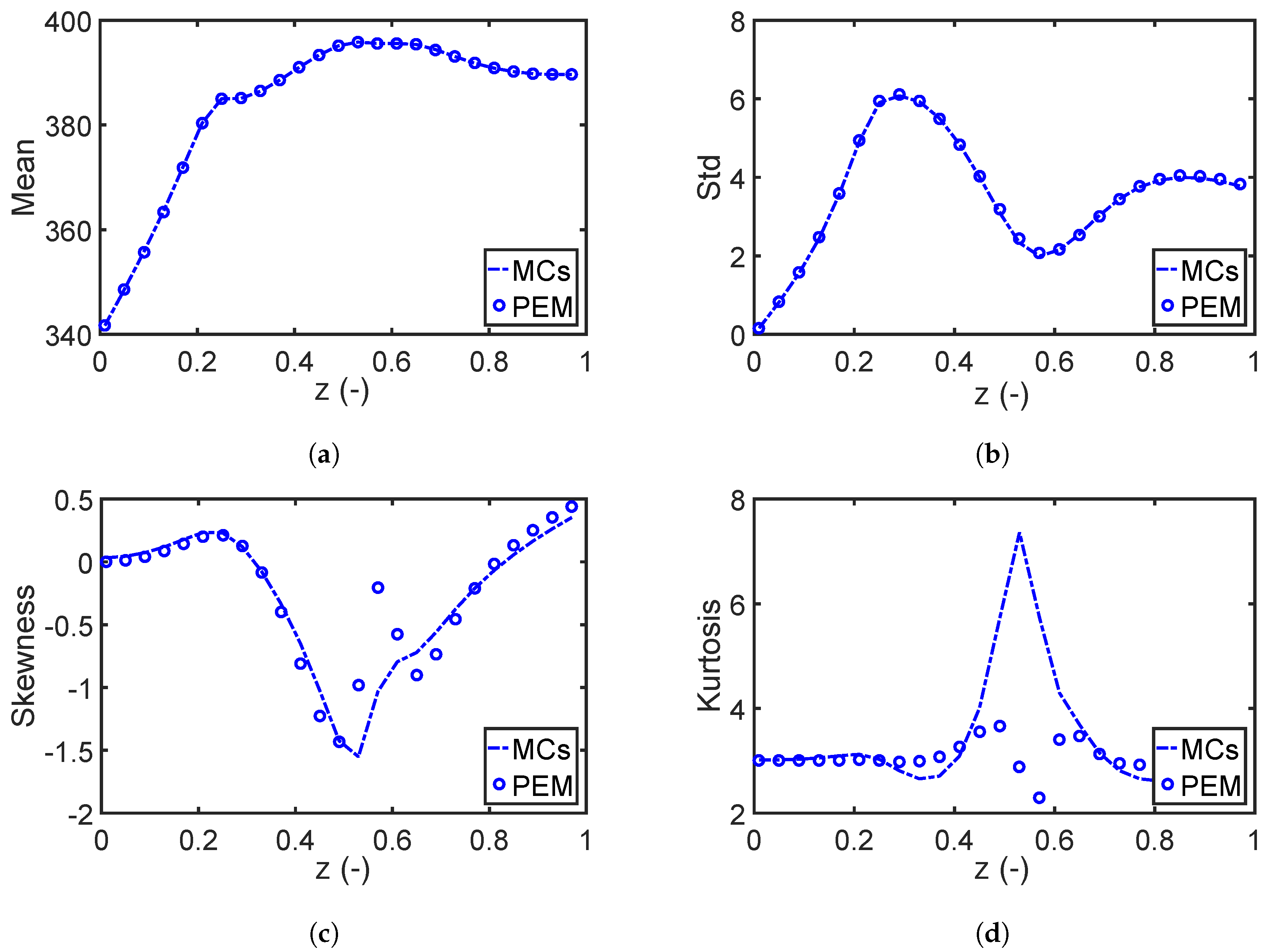
As discussed in Section 4.2, the fourth moment method uses more statistical information than the second moment method and has a lower approximation error. The same RO problem is solved again with the fourth moment approach, and the violation probabilities are estimated and listed in the right of Table 2. However, the expected improvement could not be validated. In fact, the violation probability for the correlated scenario increases in case of the fourth moment method. The reason for this unexpected performance is mainly due to the estimation error of higher order statistical moments. When we compare the first four statistical moments estimated by the PEM and the MC simulations, we can see in Figure 7 that the PEM provides useful approximations for the first and second moments and deteriorates considerably for the higher order moments. As has been mentioned, the PEM is accurate if the system can be accurately approximated with the sum of monomials up to order of five, and as such its accuracy deteriorates with the increasing order of the statistical moments. The comparison indicates that the fourth moment method might not be suitable for the PEM-based robust optimization framework, especially for practical applications where the systems might be strongly nonlinear and complex. Please note that for calculating the n-th statistical moment, not only the function $k(\xi )$ but also $k{(\xi )}^n$ has to be approximated, which is challenging for all sample-based approximation schemes, including MC simulations [2]. The fourth moment approach, in turn, is still a promising way to approximate probability distributions if the higher order moments can be estimated accurately, e.g., using polynomial chaos expansion or Gaussian mixture density approximation [61]. Based on this finding, in the following section, we exclusively implement the second moment method.

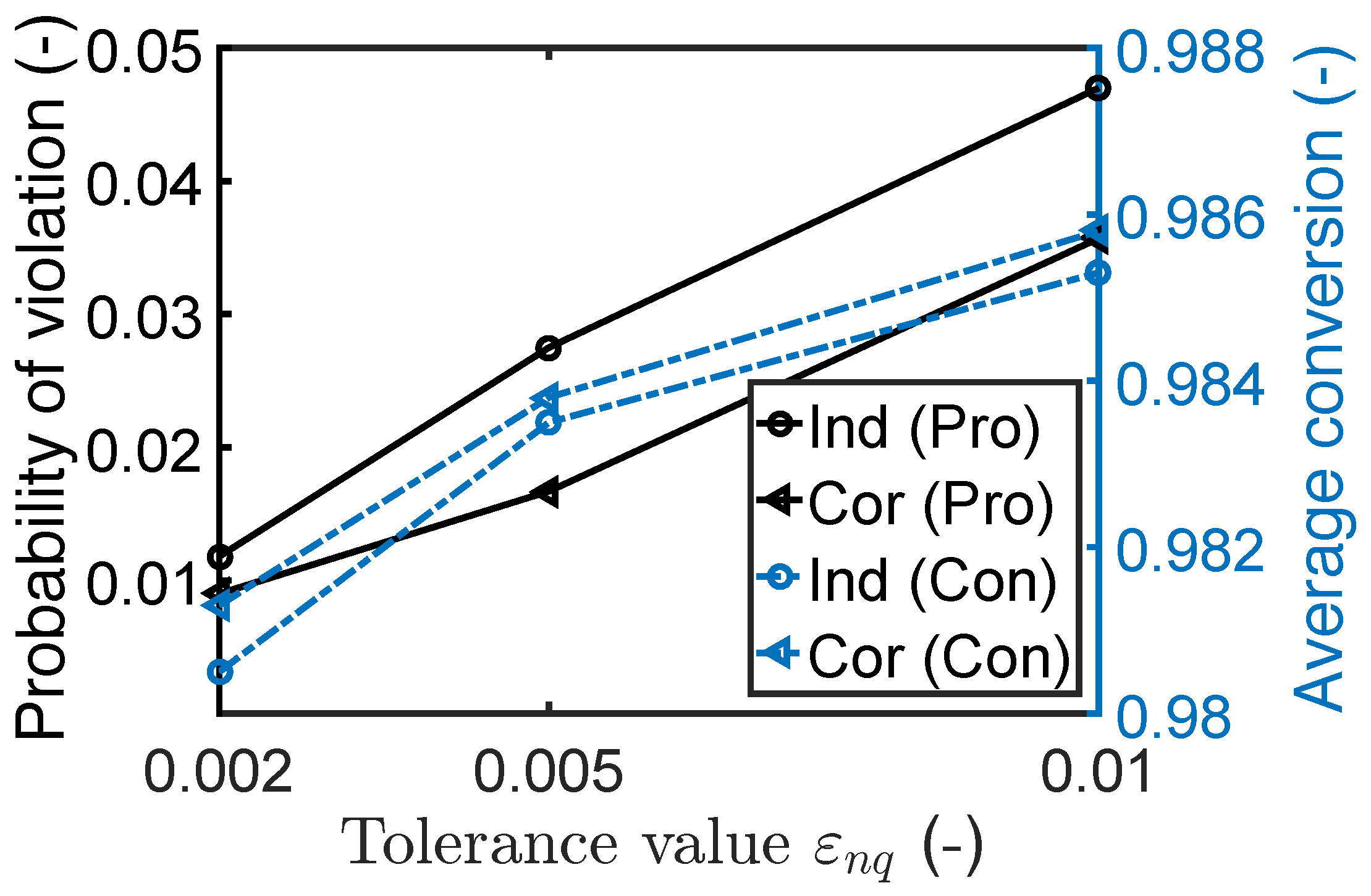
Alternatively, one might adjust the tolerance value for the robust inequality constraints to mitigate the effect of approximation errors when using the second moment method. The violation probabilities of the inequality constraints for the robust design with different tolerance values are given in Figure 8. As we can see, the probability can achieve 0.01 by setting the tolerance value to 0.002 for the independent and correlated cases, while the average conversion of reactant A was slightly impacted by changing the tolerance value; see Figure 8.

7.1.3. Impact of Robust Equality Constraints

Here, we would like to investigate the effect of robust equality constraints that might result from process specifications. The design of continuous processes follows the trend of process integration and intensification to reduce energy costs and raw material. For instance, to avoid extra cooling expenses for a downstream process, we can integrate the heat management into the reactor design directly. To this end, a terminal equality constraint is added to lower the outlet temperature to the value of the inlet temperature:

$$\left|T_r(z=1)-T_r(z=0)\right|=0.$$

(45)

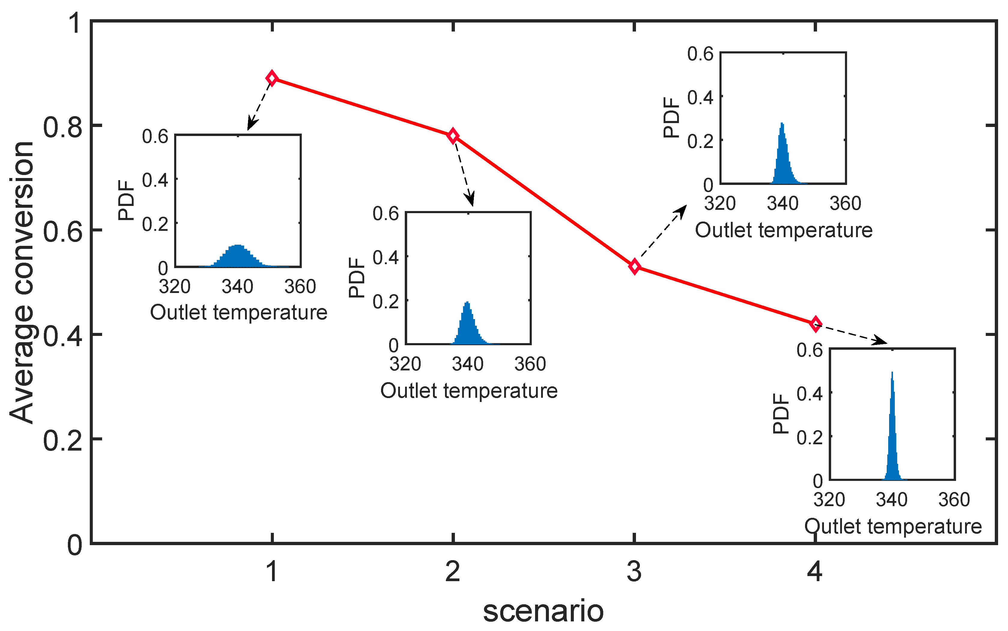
With this additional soft equality constraint, there exists a trade-off between maximizing the reactant conversion while minimizing the temperature difference. First, the results of the reactor design where we neglected parameter uncertainties are given in Figure 9a. The jacket temperature drops sharply to its lower limit for the second half of the reactor, and the outlet temperature returns exactly to 340 $\mathrm{K}$. Consequently, the reactant conversion decreases with 2% compared to the nominal design without the equality constraint (Figure 5). Next, the effect of parameter uncertainties on the nominal design is illustrated in Figure 9b with the green dotted line. Because of limited space, we mainly consider the case where uncertain parameters are correlated. In this case, a strong violation of inequality and equality constraints exists and has to be tackled properly. The robust optimization framework proposed in Section 5 is used to solve this problem. An identical setting ($\alpha =3$ and ${\epsilon }_{nq}=1\%$) is used for the objective function and inequality constraints here. Different scenarios with different relaxation factors ${\delta }_{eq}$ and tolerance factors ${\epsilon }_{eq}$ are used to demonstrate the effect of robust equality constraints on the process performance. Values for the relaxation factors and results are summarized in Figure 10. We can see that the probability distribution of the outlet temperature narrows quickly once we reduce the relaxed region and violation probability, while the performance of the reactor (the reactant conversion) deteriorates considerably. The process engineer has to decide on the trade-off between product performance and energy expense. Note that the robust inequality constraints in these scenarios are always satisfied, and thus, are not explicitly shown here.

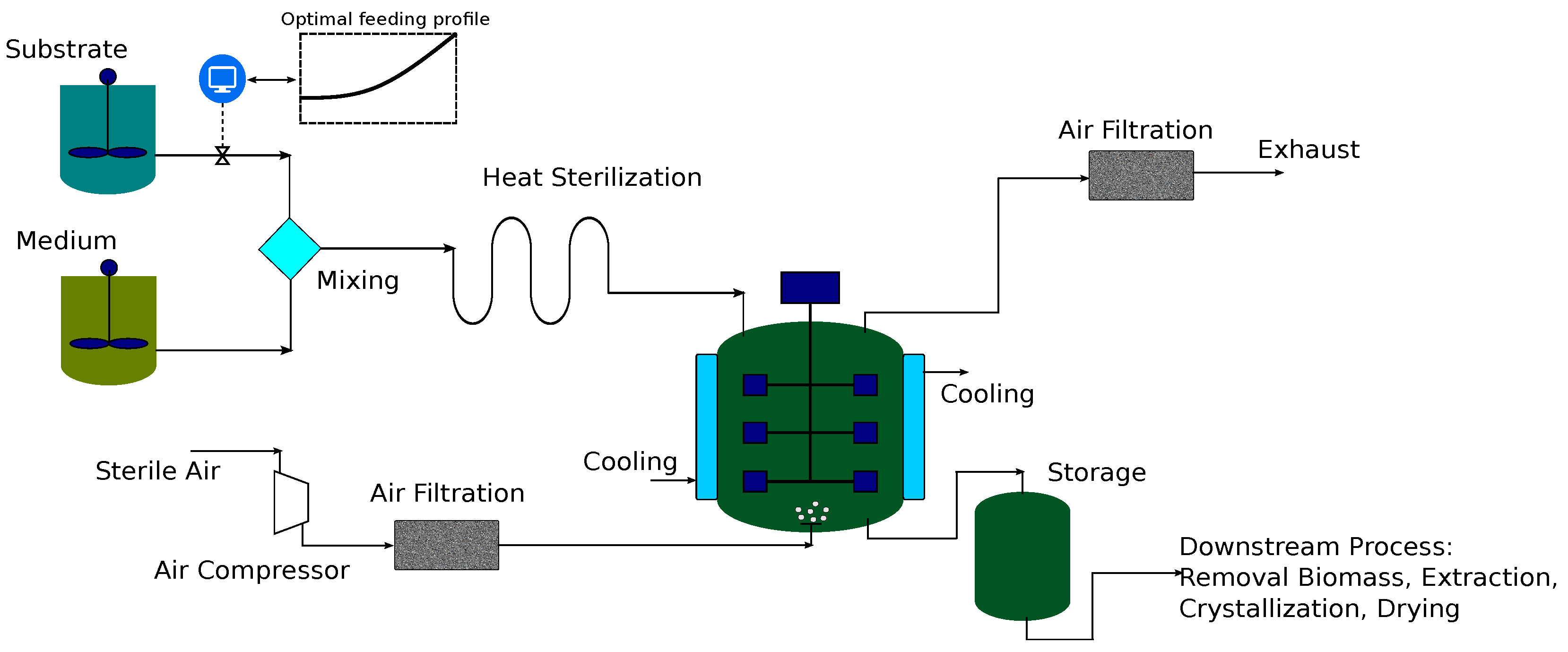
7.2. Case Study 2: Fed-Batch Bioreactor for Fermentation of Penicillin

The performance of the PEM-based robust optimization framework is also demonstrated with a fermentation process as illustrated in Figure 11. Fermentation processes have received great interest in the pharmaceutical industry, and in this study, we try to optimize the penicillin fermentation [62]. To this end, we design a feeding substrate profile that ensures the optimal performance and robustness of the bioreactor. A fed-batch reactor model is used based on the following assumptions: (1) ideal mixing of all components in the bioreactor; (2) isothermal condition in the reactor; and (3) the effect of the oxygen transfer can be neglected by considering an upper limitation on the biomass and substrate concentrations. The mathematical model for the fermentation process reads as:

$$\begin{array}{cc}\hfill & \frac{dX}{dt}=\mu X-\frac{F}{V}X\hfill \end{array}$$

(46)

$$\begin{array}{c}\frac{dS}{dt}=-\frac{\mu }{Y_x}X-\frac{{\theta }_p}{Y_p}X-m_{x}X+\frac{F}{V}(S_f-S)\hfill \end{array}$$

(47)

$$\begin{array}{c}\frac{dP}{dt}={\theta }_{p}X-KP-\frac{F}{V}P\hfill \end{array}$$

(48)

$$\begin{array}{c}\frac{dV}{dt}=F,\hfill \end{array}$$

(49)

where the state variables, $X,S,P$ and V, indicate the concentrations of the biomass, substrate, product and volume of components in the reactor, respectively. The feeding stream of the substrate has a constant concentration $S_f$ and a time-dependent flow rate F. The specific growth rate of the biomass $\mu$ and the product ${\theta }_p$ is represented by the substrate inhibition kinetic of the following form:

$$\begin{array}{cc}\hfill & \mu =\frac{{\mu }_{m}S}{S+K_{x}X}\hfill \end{array}$$

(50)

$$\begin{array}{c}{\theta }_p=\frac{{\theta }_{m}S}{S+K_p+S^2/K_i}.\hfill \end{array}$$

(51)

The initial conditions of the state variables and the nominal value of the other kinetic parameters are summarized in

Table 3. Nominal values of the model parameters and the initial conditions for the fed-batch model.

Parameters	Unit	Nominal Value	Parameters	Unit	Nominal Value
${\mu }_m$	1/h	0.11	$m_x$	1/h	0.029
$K_x$	-	0.006	$S_f$	g/L	400
${\theta }_m$	1/h	0.004	t	h	0–80
$K_p$	g/L	0.0001	$X(0)$	g/L	1
$K_i$	g/L	0.1	$S(0)$	g/L	0.5
K	1/h	0.01	$P(0)$	g/L	0
$Y_x$	-	0.47	$V(0)$	L	250
$Y_p$	-	1.2

. Further details about the model are given in [62].

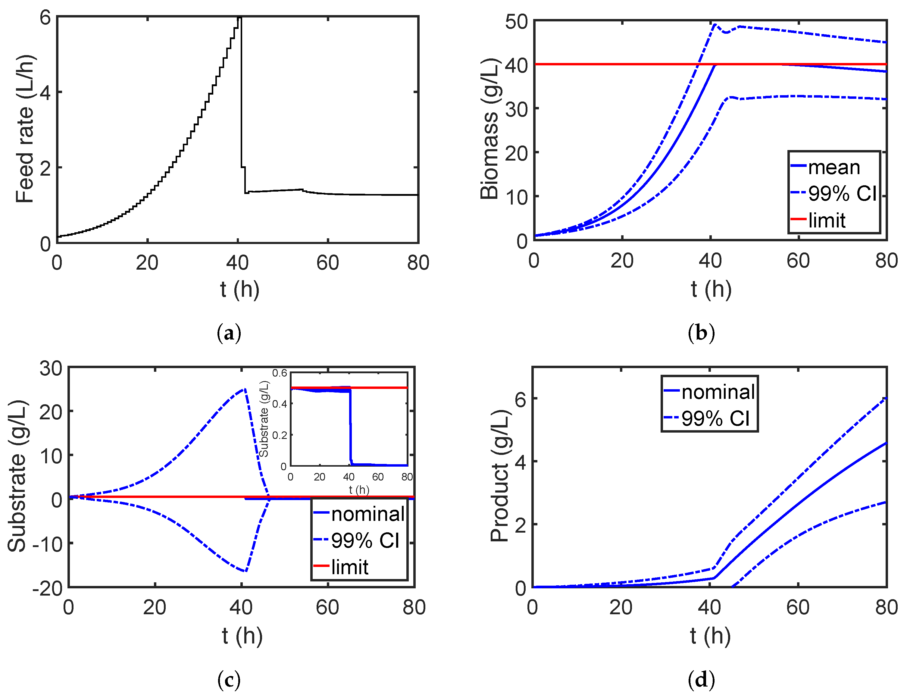
First, the process is optimized assuming that all parameters are estimated precisely; i.e., parameter uncertainties are neglected. The goal is to maximize the final concentration of product P within a given time range while the concentration of biomass X and substrate S should be below 40 g/L (limited by the oxygen transfer capacity) and 0.5 g/L (to avoid side reactions) for the entire time horizon, respectively [63]. The control variable F is parametrized with 100 elements, which are bounded within the range of [0, 10]. The resulting dynamic optimization problem is solved with the nominal value of all parameters, and the results are shown in Figure 12. Here, the feed rate of the substrate is adjusted to keep the substrate concentration equal to 0.5 g/L at which the maximum growth rate of the biomass is achieved at the beginning. After the biomass concentration reaches its upper limit, the substrate concentration drops nearly to zero to cease the self-reproduction of the biomass. Moreover, the substrate is fed at low rate that is consumed by the biomass to produce the desired product.

However, due to imperfect measurement data and model simplifications, the estimates of the model parameters may have a considerable error as well as being correlated. Based on the results given in [64], we assign the nine parameters with a multivariate normal distribution, where their marginal distributions have mean values equal to the nominal values and standard deviations equal to 10% of the nominal values. To investigate the effect of parameter correlations, two scenarios are analyzed: (1) the parameter correlations are neglected, and the correlation matrix $\Sigma$ is set to the identity matrix; (2) the correlation coefficients of ${\mu }_m,{\theta }_m,Y_x$, and $m_x$ in $\Sigma$ are set to 0.95. The effect of imprecise model parameters on the process performance is also shown in Figure 12 with the blue dotted lines. Strong violation of the constraints and large variation of the product quality are observed, and thus, the parameter uncertainty has to be considered in the process design for robustness. Please note that the negative confidence interval (CI) of the substrate concentration stems from the assumption that the CIs are symmetric and directly derived from the mean and variance of the states.

7.2.1. Global Sensitivity Analysis

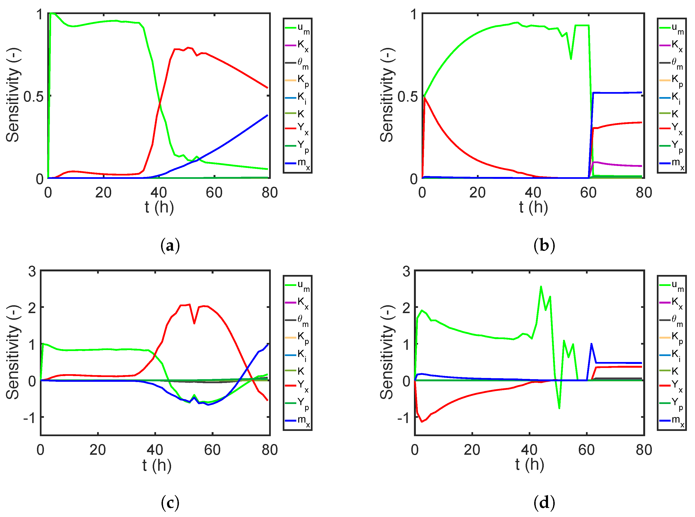
Before solving the RO problem for the fermentation process, we want to decrease its computational cost by deciding which parameters are not relevant and can be neglected in the robust process design. Thus, the corresponding time-dependent sensitivity indices of the parameters are calculated for the biomass and substrate concentrations in addition to the product concentration at the final time point, i.e., for those quantities involved in either the objective function or the constraints of the optimization problem. Figure 13a,c and Figure 14a show the sensitivity results for the independent case. As we can see, the biomass and product concentrations are strongly affected by parameters ${\mu }_m$, ${\theta }_m$, $Y_x$, and $m_x$, while the other parameters have a minor impact. Moreover, by summing up the first-order sensitivity indices, the interaction among the parameters are negligible. Next, we calculate the correlative ($S^C$) and total covariance-based ($S^{cov}$) first-order sensitivity regarding the biomass, substrate, and product concentration; see Figure 13b,d and Figure 14b. Here, we do not show the results for the structural sensitivity indices and all the total sensitivity indices. The reason is that the model structure does not change with the existence of parameter correlations, and thus, the structural sensitivity indices and parameter interactions are similar to those for the independent case. Nevertheless, an evident effect of parameter correlations on the sensitivity analysis result can be observed: The parameter sensitivities have a completely different trend compared to the independent case. The sensitivity results from the correlated case also suggest considering the uncertainties and correlations from ${\mu }_m$, ${\theta }_m$, $Y_x$, and $m_x$ for the RO problem. By using the information from the sensitivity analysis, we can significantly reduce the number of required PEM points for the RO problem. The number of model evaluations for each optimization iteration decreases from $2\times 9^2+1=163$ to $2\times 4^2+1=33$ for the independent and correlated cases. The performance of the RO with parameter uncertainties of appreciable sensitivities is studied in the following section.

7.2.2. Robust Optimization

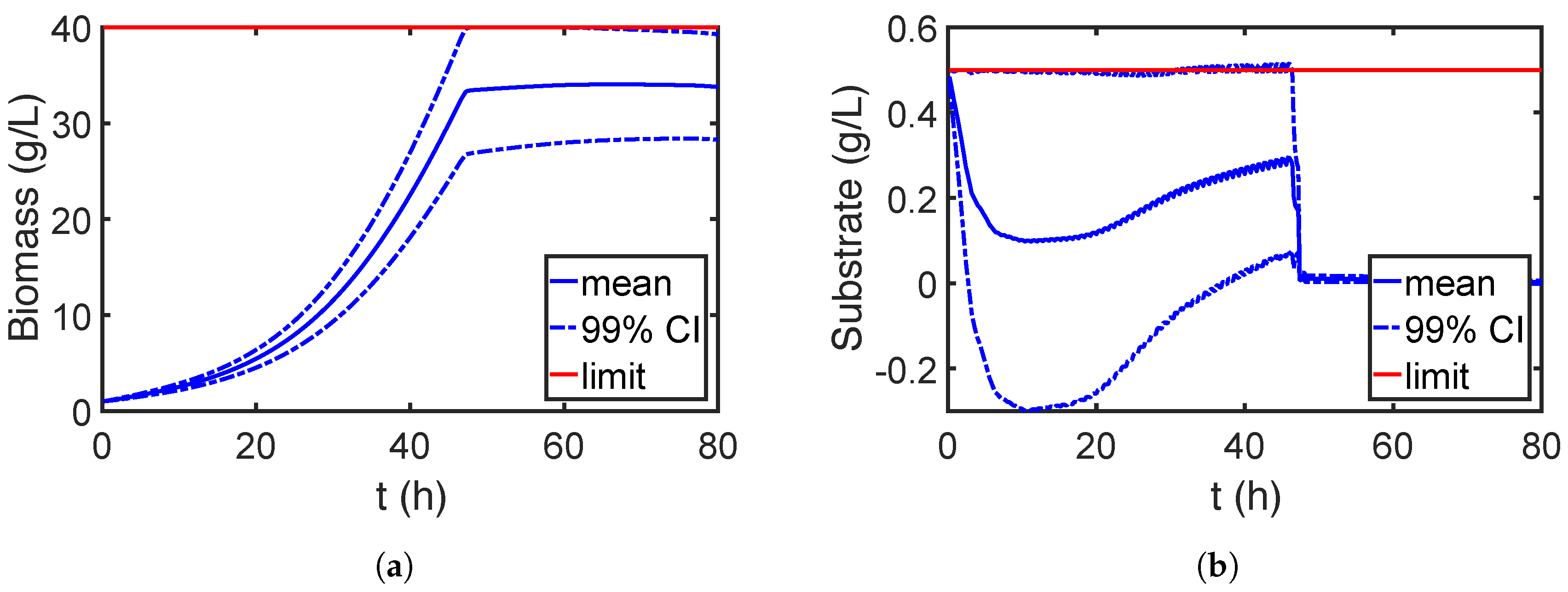
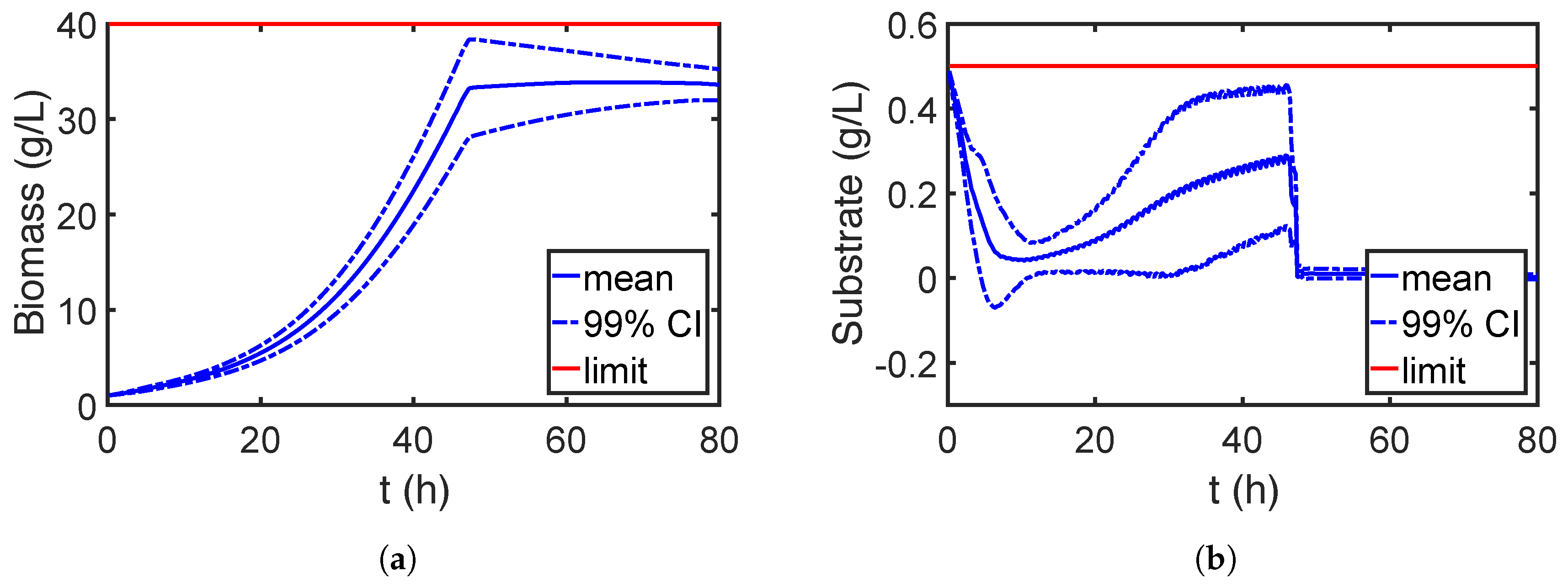
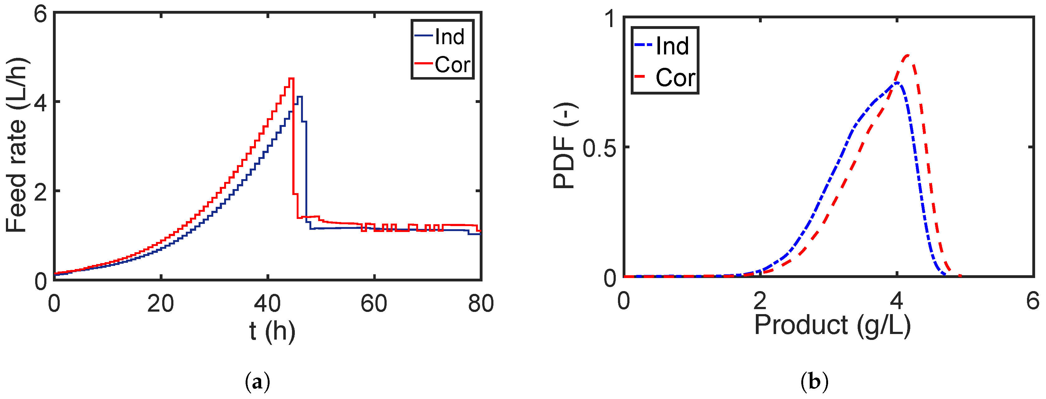
The RO is solved with the framework proposed in Section 5. To this end, a weight factor $\alpha =3$ and a tolerance value ${\epsilon }_{nq}=1\%$ are used for the robust objective and inequality constraints. The PEM points for RO are generated only for parameters with appreciable sensitivities, i.e., four parameters are considered. First, the RO is solved for the simplifying assumption of the independent parameters. The evolution of the mean and 99% CIs for the biomass and the substrate are illustrated in Figure 15. Please note that the CIs in all the plots are quantified with considering the uncertainties from all nine parameters. As we can see from Figure 15, the biomass grows rapidly until its CI approaches the upper boundary to maximize the productivity, while the CI of the substrate remains at its upper boundary at the beginning and decreases to a low value to activate the production phase. However, the result of the RO ignoring parameter dependencies is too conservative. The effect of parameter dependencies is shown in Figure 16 for the previous optimized setting, i.e., assuming independent parameters. The shape of the CIs of the biomass and the substrate are quite different from those in Figure 15 and do not reach their upper boundaries, which leaves some space for improvement. Therefore, we repeat the RO considering the parameter dependencies accordingly and show the results in Figure 17. As we can see, the CIs of both biomass and substrate concentration reach the upper boundaries and are less conservative compared to the results in Figure 16. The optimized feeding profile of the substrate for the independent and correlated cases are compared in Figure 18a. The substrate for the correlated case is fed with a higher rate and descended a bit earlier than that for the independent scenario. The PDFs of the product concentrations at the final time point shown in Figure 16 and Figure 17 are compared in more detail in Figure 18b. The product concentration is improved considerably as the dashed curve, which represents the parameter dependency case, is a bit narrowed and shifted to higher concentrations.

As mentioned above, the negative CIs of the substrate concentration in all the figures are due to the assumption of symmetric distributions of the states. This also indicates that the CIs might not be accurate, and thus, we validate them by checking the number of constraint violations with 10,000 Monte Carlo simulation for the independent and correlated case, where the corresponding optimal feeding profiles are applied. The results are listed in

Table 4. The number of constraint violations from 10,000 Monte Carlo simulations, where the tolerance factor ${\epsilon }_{nq}=1\%$ and ${\epsilon }_{nq}=0.14\%$ for both designs with independent and correlated parameters. The performance indicates the mean value of the production concentration at the end.

		Independent	Correlated
${\epsilon }_{nq}=1\%$	X	146	35
	S	572	554
performance		3.63	3.76
${\epsilon }_{nq}=0.14\%$	X	19	2
	S	378	369
performance		3.53	3.67

. As we can see from the second row, the violation frequencies are higher than expected, ${\epsilon }_{nq}=1\%=\frac{100}{10,000}$, especially for the substrate concentration. Although the violation frequencies might be acceptable for practical applications, we can improve the RO credibility by using a smaller tolerance factor as introduced in Section 7.1.2. Corresponding results are shown in the third row of Table 4. All violation numbers are improved, while we slightly lower the reactor performance regarding the penicillin productivity.

8. Conclusions

In this work, we proposed a new framework for solving robust optimization problems using the point estimate method. Here, a sampling strategy derived from an isoprobabilistic transformation was used to include parameter dependencies and soft equality constraints of practical relevance. In parallel, we also analyzed methods including fourth-order statistical moments to approximate robust equality and inequality constraints. To include only the most relevant model parameters and to reduce the computation costs, we also calculated the global parameter sensitivities before the robustification step.

Two case studies, which include chemical and biological production processes, were used to demonstrate the performance of the proposed framework. The first case study attempts to maximize the conversion of a reactant while simultaneously satisfying the constraints on the reactor temperature of a tubular reactor. The proposed method addresses the trade-off between performance and robustness for the reactor under parameter uncertainties. We observed an evident influence of parameter correlation on the designed control profile and confidence intervals of the system states. Performances of the second and fourth moment methods for approximating the robust inequality constraints were also examined. The fourth moment method has a more rigorous structure compared to the second moment approach. However, the performance of the fourth moment method is limited by the accuracy of the PEM. Thus, we concluded that the second moment method might be more favorable in this particular case. Furthermore, the approximation error could be compensated by using more conservative tolerance values, which resulted in slight deterioration of the reactor performance. To save energy costs, we also added an equality constraint to the outlet temperature. The robust equality constraint had to be relaxed deliberately to be solvable. The process performance deteriorated dramatically with lower relaxation factors. The second example is the optimal design of a bioreactor for a penicillin fermentation process. Global sensitivity analysis was used to determine the relevant parameters and to ease the computational expense of the robustification framework. This is extremely useful for large-scale problems with a high number of uncertain parameters. Moreover, the effect of parameter correlations on the robust process design was also observed. Here, the PEM still performs reasonably well and retains a relatively low computational cost.

In conclusion, the proposed framework provides a comprehensive strategy for robust optimization problems and covers features that have not been considered in previous works. It is able to achieve suitable robust design in the absence and presence of parameter correlations at low computational costs. As discussed, the PEM might fail in estimating higher order statistical moments, especially for systems with strong nonlinearities. This is also the main reason why the performance of the fourth moment method did not provide the expected improvement in robustification. Alternatively, the accuracy of the PEM can be increased using extended sample-generating rules, i.e., higher sample number results in more precise approximation at the cost of efficiency, or different methods for uncertainty quantification might be studied. Future work will focus on this issue.

References

- Biegler, L.T. Nonlinear Programming: Concepts, Algorithms, and Applications To Chemical Processes; SIAM: Philadelphia, PA, USA, 2010. [Google Scholar]
- Schenkendorf, R. Optimal Experimental Design for Paramter Identification and Model Selection. Ph.D. Thesis, Otto-von-Guericke-Universität Magdeburg, Magdeburg, Germany, 2014. [Google Scholar]
- Mortier, S.T.F.; Van Bockstal, P.J.; Corver, J.; Nopens, I.; Gernaey, K.V.; De Beer, T. Uncertainty analysis as essential step in the establishment of the dynamic Design Space of primary drying during freeze-drying. Eur. J. Pharm. Biopharm. 2016, 103, 71–83. [Google Scholar] [CrossRef] [PubMed] [Green Version]
- Taguchi, G.; Clausing, D. Robust quality. Harv. Bus. Rev. 1990, 68, 65–75. [Google Scholar]
- Vallerio, M.; Telen, D.; Cabianca, L.; Manenti, F.; Van Impe, J.; Logist, F. Robust multi-objective dynamic optimization of chemical processes using the Sigma Point method. Chem. Eng. Sci. 2016, 140, 201–216. [Google Scholar] [CrossRef] [Green Version]
- Xie, X.; Schenkendorf, R.; Krewer, U. Robust design of chemical processes based on a one-shot sparse polynomial chaos expansion concept. Comput. Aided Chem. Eng. 2017, 40, 613–618. [Google Scholar]
- Nagy, Z.K.; Braatz, R.D. Worst-case and distributional robustness analysis of finite-time control trajectories for nonlinear distributed parameter systems. IEEE Trans. Control Syst. Technol. 2003, 11, 694–704. [Google Scholar] [CrossRef]
- Ghaoui, L.E.; Oks, M.; Oustry, F. Worst-case value-at-risk and robust portfolio optimization: A conic programming approach. Oper. Res. 2003, 51, 543–556. [Google Scholar] [CrossRef]
- Janak, S.L.; Lin, X.; Floudas, C.A. A new robust optimization approach for scheduling under uncertainty: II. Uncertainty with known probability distribution. Comput. Chem. Eng. 2007, 31, 171–195. [Google Scholar] [CrossRef]
- Venter, G.; Haftka, R. Using response surface approximations in fuzzy set based design optimization. Struct. Multidiscipl. Optim. 1999, 18, 218–227. [Google Scholar] [CrossRef]
- Beyer, H.G.; Sendhoff, B. Robust optimization–a comprehensive survey. Comput. Methods Appl. Mech. Eng. 2007, 196, 3190–3218. [Google Scholar] [CrossRef]
- Smith, R.C. Uncertainty Quantification: Theory, Implementation, And Applications; SIAM: Philadelphia, PA, USA, 2013; Volume 12. [Google Scholar]
- Shi, J.; Biegler, L.T.; Hamdan, I.; Wassick, J. Optimization of grade transitions in polyethylene solution polymerization process under uncertainty. Comput. Chem. Eng. 2016, 95, 260–279. [Google Scholar] [CrossRef]
- Wiener, N. The homogeneous chaos. Am. J. Math. 1938, 60, 897–936. [Google Scholar] [CrossRef]
- Xiu, D.; Karniadakis, G.E. The Wiener–Askey polynomial chaos for stochastic differential equations. SIAM J. Sci. Comput. 2002, 24, 619–644. [Google Scholar] [CrossRef]
- Mesbah, A.; Streif, S. A probabilistic approach to robust optimal experiment design with chance constraints. IFAC-PapersOnLine 2015, 48, 100–105. [Google Scholar] [CrossRef]
- Nimmegeers, P.; Telen, D.; Logist, F.; Van Impe, J. Dynamic optimization of biological networks under parametric uncertainty. BMC Syst. Biol. 2016, 10, 86. [Google Scholar] [CrossRef] [PubMed]
- Paulson, J.A.; Mesbah, A. An efficient method for stochastic optimal control with joint chance constraints for nonlinear systems. Int. J. Robust Nonlinear Control 2017. [Google Scholar] [CrossRef]
- Golub, G.H.; Welsch, J.H. Calculation of Gauss quadrature rules. Math. Comput. 1969, 23, 221–230. [Google Scholar] [CrossRef]
- Xie, X.; Krewer, U.; Schenkendorf, R. Robust Optimization of Dynamical Systems with Correlated Random Variables using the Point Estimate Method. IFAC-PapersOnLine 2018, 51, 427–432. [Google Scholar] [CrossRef]
- Freund, H.; Maußner, J. Optimization Under Uncertainty in Chemical Engineering: Comparative Evaluation of Unscented Transformation Methods and Cubature Rules. Chem. Eng. Sci. 2018, 183, 329–345. [Google Scholar]
- Saltelli, A.; Chan, K.; Scott, E.M. Sensitivity Analysis; Wiley: New York, NY, USA, 2000; Volume 1. [Google Scholar]
- Reizman, B.J.; Jensen, K.F. An automated continuous-flow platform for the estimation of multistep reaction kinetics. Org. Process Res. Dev. 2012, 16, 1770–1782. [Google Scholar] [CrossRef]
- Sudret, B.; Caniou, Y. Analysis of covariance (ANCOVA) using polynomial chaos expansions. In Proceedings of the 11th International Conference on Structural Safety & Reliability, New York, NY, USA, 16–20 June 2013. [Google Scholar]
- Valkó, É.; Varga, T.; Tomlin, A.; Busai, Á.; Turányi, T. Investigation of the effect of correlated uncertain rate parameters via the calculation of global and local sensitivity indices. J. Math. Chem. 2018, 56, 864–889. [Google Scholar] [CrossRef]
- López-Benito, A.; Bolado-Lavín, R. A case study on global sensitivity analysis with dependent inputs: The natural gas transmission model. Reliab. Eng. Syst. Saf. 2017, 165, 11–21. [Google Scholar] [CrossRef]
- Valkó, É.; Varga, T.; Tomlin, A.; Turányi, T. Investigation of the effect of correlated uncertain rate parameters on a model of hydrogen combustion using a generalized HDMR method. Proc. Combust. Inst. 2017, 36, 681–689. [Google Scholar] [CrossRef] [Green Version]
- Xie, X.; Ohs, R.; Spieß, A.; Krewer, U.; Schenkendorf, R. Moment-Independent Sensitivity Analysis of Enzyme-Catalyzed Reactions with Correlated Model Parameters. IFAC-PapersOnLine 2018, 51, 753–758. [Google Scholar] [CrossRef]
- Lebrun, R.; Dutfoy, A. Do Rosenblatt and Nataf isoprobabilistic transformations really differ? Probab. Eng. Mech. 2009, 24, 577–584. [Google Scholar] [CrossRef]
- Logist, F.; Smets, I.; Van Impe, J. Derivation of generic optimal reference temperature profiles for steady-state exothermic jacketed tubular reactors. J. Process Control 2008, 18, 92–104. [Google Scholar] [CrossRef]
- Telen, D.; Vallerio, M.; Cabianca, L.; Houska, B.; Van Impe, J.; Logist, F. Approximate robust optimization of nonlinear systems under parametric uncertainty and process noise. J. Process Control 2015, 33, 140–154. [Google Scholar] [CrossRef] [Green Version]
- Zhao, Y.G.; Ono, T. Moment methods for structural reliability. Struct. Saf. 2001, 23, 47–75. [Google Scholar] [CrossRef]
- Chaloner, K.; Verdinelli, I. Bayesian experimental design: A review. Stat. Sci. 1995, 10, 273–304. [Google Scholar] [CrossRef]
- Lerner, U.N. Hybrid Bayesian Networks for Reasoning About Complex Systems. Ph.D. Thesis, Stanford University Stanford, Stanford, CA, USA, 2002. [Google Scholar]
- Schenkendorf, R. A general framework for uncertainty propagation based on point estimate methods. In Proceedings of the Second european conference of the prognostics and health management society, phme14, Nantes, France, 8–10 July 2014. [Google Scholar]
- Maußner, J.; Freund, H. Optimization under uncertainty in chemical engineering: Comparative evaluation of unscented transformation methods and cubature rules. Chem. Eng. Sci. 2018, 183, 329–345. [Google Scholar] [CrossRef]
- Julier, S.J.; Uhlmann, J.K. A General Method for Approximating Nonlinear Transformations of Probability Distributions; Robotics Research Group, Department of Engineering Science, University of Oxford: Oxford, UK, 1996. [Google Scholar]
- Schenkendorf, R.; Groos, J.C. Global sensitivity analysis applied to model inversion problems: A contribution to rail condition monitoring. Int. J. Progn. Health Manag. 2015, 6, 1–14. [Google Scholar]
- Schenkendorf, R.; Mangold, M. Qualitative and quantitative optimal experimental design for parameter identification of a map kinase model. IFAC Proc. Vol. 2011, 44, 11666–11671. [Google Scholar] [CrossRef]
- Telen, D.; Logist, F.; Van Derlinden, E.; Van Impe, J.F. Robust optimal experiment design: A multi-objective approach. IFAC Proc. Vol. 2012, 45, 689–694. [Google Scholar] [CrossRef]
- Schenkendorf, R.; Xie, X.; Rehbein, M.; Scholl, S.; Krewer, U. The Impact of Global Sensitivities and Design Measures in Model-Based Optimal Experimental Design. Processes 2018, 6, 27. [Google Scholar] [CrossRef]
- Lebrun, R.; Dutfoy, A. A generalization of the Nataf transformation to distributions with elliptical copula. Probab. Eng. Mech. 2009, 24, 172–178. [Google Scholar] [CrossRef]
- Rangavajhala, S.; Mullur, A.; Messac, A. The challenge of equality constraints in robust design optimization: Examination and new approach. Struct. Multidiscipl. Optim. 2007, 34, 381–401. [Google Scholar] [CrossRef]
- Ostrovsky, G.; Ziyatdinov, N.; Lapteva, T. Optimal design of chemical processes with chance constraints. Comput. Chem. Eng. 2013, 59, 74–88. [Google Scholar] [CrossRef]
- Kolmogorov, A.N. Foundations of the Theory of Probability: Second English Edition; Courier Dover Publications: Mineola, NY, USA, 2018. [Google Scholar]
- Smola, A.J.; Schölkopf, B. A tutorial on support vector regression. Stat. Comput. 2004, 14, 199–222. [Google Scholar] [CrossRef] [Green Version]
- Boukouvala, F.; Niotis, V.; Ramachandran, R.; Muzzio, F.J.; Ierapetritou, M.G. An integrated approach for dynamic flowsheet modeling and sensitivity analysis of a continuous tablet manufacturing process. Comput. Chem. Eng. 2012, 42, 30–47. [Google Scholar] [CrossRef]
- Rehrl, J.; Gruber, A.; Khinast, J.G.; Horn, M. Sensitivity analysis of a pharmaceutical tablet production process from the control engineering perspective. Int. J. Pharm. 2017, 517, 373–382. [Google Scholar] [CrossRef] [PubMed]
- Kiparissides, A.; Kucherenko, S.; Mantalaris, A.; Pistikopoulos, E. Global sensitivity analysis challenges in biological systems modeling. Ind. Eng. Chem. Res. 2009, 48, 7168–7180. [Google Scholar] [CrossRef]
- Wang, Z.; Ierapetritou, M. Global sensitivity, feasibility, and flexibility analysis of continuous pharmaceutical manufacturing processes. Comput. Aided Chem. Eng. 2018, 41, 189–213. [Google Scholar]
- Lin, N.; Xie, X.; Schenkendorf, R.; Krewer, U. Efficient global sensitivity analysis of 3D multiphysics model for Li-ion batteries. J. Electrochem. Soc. 2018, 165, A1169–A1183. [Google Scholar] [CrossRef]
- Li, G.; Rabitz, H.; Yelvington, P.E.; Oluwole, O.O.; Bacon, F.; Kolb, C.E.; Schoendorf, J. Global sensitivity analysis for systems with independent and/or correlated inputs. J. Phys. Chem. A 2010, 114, 6022–6032. [Google Scholar] [CrossRef] [PubMed]
- Mara, T.A.; Tarantola, S.; Annoni, P. Non-parametric methods for global sensitivity analysis of model output with dependent inputs. Environ. Model. Softw. 2015, 72, 173–183. [Google Scholar] [CrossRef]
- Borgonovo, E. A new uncertainty importance measure. Reliab. Eng. Syst. Saf. 2007, 92, 771–784. [Google Scholar] [CrossRef]
- Xie, X.; Schenkendorf, R.; Krewer, U. Efficient sensitivity analysis and interpretation of parameter correlations in chemical engineering. Reliab. Eng. Syst. Saf. 2018. [Google Scholar] [CrossRef]
- Marelli, S.; Sudret, B. UQLab: A framework for uncertainty quantification in Matlab. In Proceedings of the Second International Conference on Vulnerability and Risk Analysis and Management (ICVRAM) and the Sixth International Symposium on Uncertainty, Modeling, and Analysis (ISUMA), Liverpool, UK, 13–16 July 2014; pp. 2554–2563. [Google Scholar]
- Biegler, L.T. An overview of simultaneous strategies for dynamic optimization. Chem. Eng. Process. Process Intensif. 2007, 46, 1043–1053. [Google Scholar] [CrossRef]
- Andersson, J.; Åkesson, J.; Diehl, M. CasADi: A symbolic package for automatic differentiation and optimal control. In Recent Advances in Algorithmic Differentiation; Springer: New York, NY, USA, 2012; pp. 297–307. [Google Scholar]
- Wächter, A.; Biegler, L.T. On the implementation of an interior-point filter line-search algorithm for large-scale nonlinear programming. Math Program 2006, 106, 25–57. [Google Scholar] [CrossRef]
- Duff, I.S. MA57—A code for the solution of sparse symmetric definite and indefinite systems. ACM Trans. Math. Softw. (TOMS) 2004, 30, 118–144. [Google Scholar] [CrossRef]
- Rossner, N.; Heine, T.; King, R. Quality-by-design using a gaussian mixture density approximation of biological uncertainties. IFAC Proc. Vol. 2010, 43, 7–12. [Google Scholar] [CrossRef]
- Bajpai, R.; Reuss, M. A mechanistic model for penicillin production. J. Chem. Technol. Biotechnol. 1980, 30, 332–344. [Google Scholar] [CrossRef]
- San, K.Y.; Stephanopoulos, G. Optimization of fed-batch penicillin fermentation: A case of singular optimal control with state constraints. Biotechnol. Bioeng. 1989, 34, 72–78. [Google Scholar] [CrossRef] [PubMed]
- Chu, Y.; Hahn, J. Necessary condition for applying experimental design criteria to global sensitivity analysis results. Comput. Chem. Eng. 2013, 48, 280–292. [Google Scholar] [CrossRef]
Figure 1.
Computational demand (i.e., number of model evaluations) for different uncertainty quantification methods with increasing number of uncertain parameters and the same system complexity to achieve similar approximation accuracy.
Figure 2.
Illustration of the point estimation method (PEM) for a nonlinear function that has (A) two random inputs; (B) one model output ; and (C) the resulting approximations of statistical moments of .
Figure 3.
Illustration of soft equality constraints . For the sake of explanation, a two-dimensional random space with uncertain parameters and is used. Samples satisfying the constraints are shown by blue-filled circles ●, while samples that violate the constraints are shown by red cross ⨯. (a) The probability of samples that satisfy the equality constraint (red line —) is equal to zero for the continuous random space; (b) the equality constraint and its relaxed boundaries (green dashed line - -) with width . The probability of satisfying the equality constraints is given by the percentage of samples, i.e., ●, which are located within the boundaries.
Figure 4.
Structure of sensitivity measures for independent (left) and correlated (right) parameters.
Figure 5.
Results for nominal design (left) and robust design (right). (a,b) are the optimal profiles of the jacket temperature; (c,d) are the evolution of the reactor temperature and the 99% confidence interval (CI). The mean and standard deviation of the conversion of reactant A have values of [0.996, 0.004] and [0.985, 0.010] for the nominal and robust design, respectively.
Figure 6.
Results for robust design with parameter correlation: (a) the optimal jacket temperature profile and (b) the reactor temperature and its 99% confidence interval (CI). The mean and standard deviation of the conversion of reactant A are 0.986 and 0.008, respectively.
Figure 7.
A comparison of the first four statistical moments, (a) mean value, (b) standard deviation, (c) skewness, and (d) kurtosis, estimated with the point estimate method (PEM) and Monte Carlo (MC) simulations for the reactor temperature in Case Study 1.
Figure 8.
The violation probability of the reactor temperature (Pro) and the average conversion of the reactant A (Con) for process designs with different tolerance values. Ind and Cor indicate the results for the independent and correlated scenarios.
Figure 9.
Results for the nominal design with terminal equality constraints: (a) the optimal jacket temperature profile and (b) the reactor temperature with its 99% confidence interval (CI). The mean and standard deviation of the conversion of reactant A are 0.980 and 0.016, respectively.
Figure 10.
The average conversion of reactant A and the probability density function of the outlet temperature for four scenarios that have different relaxation factors and tolerance factors . 1: , 2: , 3: , 4: .
Figure 11.
Scheme of a fermentation process with a fed-batch bioreactor.
Figure 12.
(a) Feeding profile; evolution of the (b) biomass; (c) substrate and (d) product obtained from the nominal design, where the parameter uncertainties are neglected. In turn, the blue dotted lines illustrate the effect of the parameter uncertainties.
Figure 13.
Sensitivity results of the nine parameters on the biomass and substrate concentrations for the independent case: (a) first-order sensitivity indices for the concentration of biomass X; (b) first-order sensitivity indices for the concentration of substrate S; and correlated case (c) total covariance-based first-order sensitivity indices for biomass X; (d) total covariance-based first-order sensitivity indices for substrate S.
Figure 14.
Sensitivity results of nine parameters on the final product concentrations for the independent (a) and correlated (b) case.
Figure 15.
Evolution of the mean and 99% confidence interval (CI) of the (a) biomass and (b) substrate concentrations for the robust design of the fed-batch bioreactor, where the uncertain parameters are independent. The feeding profile from the robust design with independent uncertain parameters is applied.
Figure 16.
Evolution of the mean and 99% confidence interval (CI) of the (a) biomass and (b) substrate concentrations for the robust design of the fed-batch bioreactor, where the uncertain parameters are correlated. The feeding profile from the robust design with independent uncertain parameters is applied.
Figure 17.
Evolution of the mean and 99% confidence interval (CI) of the (a) biomass and (b) substrate concentrations for the robust design of the fed-batch bioreactor, where the uncertain parameters are correlated. The feeding profile from the robust design with correlated uncertain parameters is applied.
Figure 18.
Results for the robust design of the fed-batch bioreactor, where the uncertain parameters are either independent or correlated. (a) control sequence for substrate feeding; and (b) final concentration of the product, respectively.