1. Introduction
In the process industries, performing model-based optimization to obtain economic operations usually implies the need of handling the problem of plant-model mismatch. An optimum that is calculated using a theoretical model seldom represents the plant optimum. As a result, real-time optimization (RTO) is attracting considerable industrial interest. RTO is a model based upper-level optimization system that is operated iteratively in closed loop and provides set-points to the lower-level regulatory control system in order to maintain the process operation as close as possible to the economic optimum. RTO schemes usually estimate the process states and some model parameters or disturbances from the measured data but employ a fixed process model which leads to problems if the model does not represent the plant accurately.
Several schemes have been proposed towards how to combine the use of theoretical models and of the collected data during process operation, in particular the model adaptation or two-step scheme [
1]. It handles plant-model mismatch in a sequential manner via an identification step followed by an optimization step. Measurements are used to estimate the uncertain model parameters, and the updated model is used to compute the decision variables via model-based optimization. The model adaptation approach is expected to work well when the plant-model mismatch is only of parametric nature, and the operating conditions lead to sufficient excitation for the estimation of the plant outputs. In practice, however, both parametric and structural mismatch are typically present and, furthermore, the excitation provided by the previously visited operating points is often not sufficient to accurately identify the model parameters.
For an RTO scheme to converge to the plant optimum, it is necessary that the gradients of the objective as well as the values and gradients of the constraints of the optimization problem match those of the plant. Schemes that directly adapt the model-based optimization problem by using the update terms (called modifiers) which are computed from the collected data have been proposed [
2,
3,
4]. The modifier-adaptation schemes can handle considerable plant-model mismatch by applying bias- and gradient-corrections to the objective and to the constraint functions. One of the major challenges in practice, as shown in [
5], is the estimation of the plant gradients with respect to the decision variables from noisy measurement data.
Gao et al. [
6] combined the idea of modifier adaptation with the quadratic approximation approach that is used in derivative-free optimization and proposed the modifier adaptation with quadratic approximation (in short MAWQA) algorithm. Quadratic approximations of the objective function and of the constraint functions are constructed based on the screened data which are collected during the process operation. The plant gradients are computed from the quadratic approximations and are used to adapt the objective and the constraint functions of the model-based optimization problem. Simulation studies for the optimization of a reactor benchmark problem with noisy data showed that by performing some explorative moves the true optimum can be reliably obtained. However, neither the generation of the explorative moves nor their necessity for the convergence of set-point to the optimum was theoretically studied. Due to the fact that the estimation of the gradients using the quadratic approximation approach requires more data than those that are required by using a finite difference approach, the efficiency of the MAWQA algorithm, in terms of the number of plant evaluations to obtain the optimum, has been questioned, in particular for the case of several decision variables. In addition, in practice, it is crucial for plant operators to be confident with the necessity of taking the explorative moves which may lead to a deterioration of plant performance.
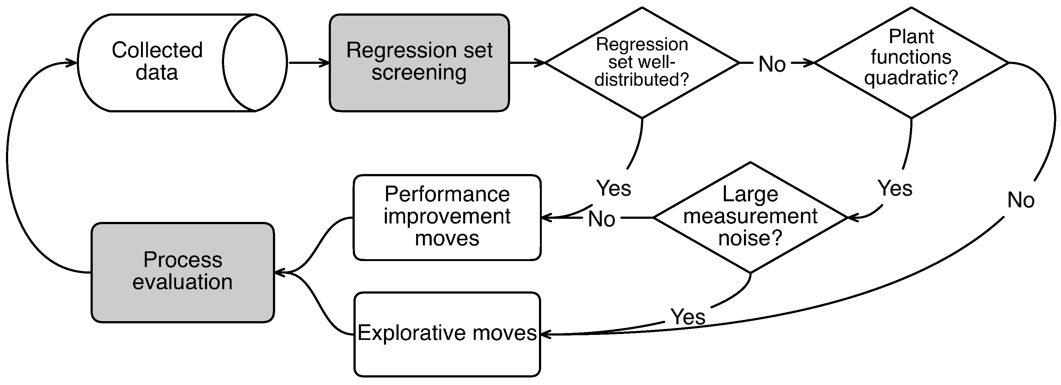
This paper reports a detailed study of the explorative moves during modifier adaptation with quadratic approximation. It starts with how the explorative moves are generated and then the factors that influence the generation of these moves are presented. The causality between the factors and the explorative moves is depicted in
Figure 1, where the blocks with a yellow background represent the factors. The use of a screening algorithm to optimize the regression set for quadratic approximations is shown to ensure that an explorative move is only performed when the past collected data cannot provide accurate gradient estimates. Simulation results for the optimization of a hydroformylation process with four optimization variables are used to illustrate the efficiency of the MAWQA algorithm, which takes necessary explorative moves, over the finite difference based modifier adaptation algorithm.
2. Modifier Adaptation with Quadratic Approximation
Let
and
represent the objective and the vector of constraint functions of a static model-based optimization problem, assumed to be twice differentiable with respect to the vector of decision variables
At each iteration of the modifier adaptation algorithm, bias- and gradient-corrections of the optimization problem are applied as
The symbols are explained in
Table 1.
and
are usually approximated by the finite difference approach
where
is the number of dimensions of
,
,
, are the plant objectives at set-points
,
, and
is approximated similarly. The accuracy of the finite difference approximations is influenced by both the step-sizes between the set-points and the presence of measurement noise. In order to acquire accurate gradient estimations, small step-sizes are preferred. However, the use of small step-sizes leads to a high sensitivity of the gradient estimates to measurement noise.
In the MAWQA algorithm, the gradients are computed analytically from quadratic approximations of the objective function and of the constraint functions that are regressed based on a screened set (represented by
at the
kth iteration) of all the collected data (represented by
). The screened set consists of near and distant points:
, where
, and
is determined by
where
is sufficiently large so that
guarantees robust quadratic approximations with noisy data,
is the minimal angle between all possible vectors that are defined by
, and
is the number of data required to uniquely determine the quadratic approximations.
In the MAWQA algorithm, the regression set
is also used to define a constrained search space
for the next set-point move
where
is the covariance matrix of the selected points (inputs) and
γ is a scaling parameter.
is a
-axial ellipsoid centered at
. The axes of the ellipsoid are thus aligned with the eigenvectors of the covariance matrix. The semi-axis lengths of the ellipsoid are related to the eigenvalues of the covariance matrix by the scaling parameter
γ. The adapted optimization (
2) is augmented by the search space constraint as
where
and
represent the adapted objective and constraint functions in (
2).
In the application of the modifier adaptation with quadratic approximation, it can happen that the nominal model is inadequate for the modifier-adaptation approach and that it is better to only use the quadratic approximations to compute the next plant move. In order to ensure the convergence, it is necessary to monitor the performance of the adapted optimization and possibly to switch between model-based and data-based optimizations. In each iteration of the MAWQA algorithm, a quality index of the adapted optimization
is calculated and compared with the quality index of the quadratic approximation
, where
and
with
and
are the quadratic approximations of the objective and the constraint functions. If
, the predictions of the adapted model-based optimization are more accurate than that of the quadratic approximations and (
6) is performed to determine the next set-point. Otherwise, an optimization based on the quadratic approximations is done
The MAWQA algorithm is given as follows:
- Step 1.
Choose an initial set-point
and probe the plant at
and
, where
h is a suitable step size and
are mutually orthogonal unit vectors. Use the finite difference approach to calculate the gradients at
and run the IGMO approach [
3] until
set-points have been generated. Run the screening algorithm to define the regression set
. Initialize
and
.
- Step 2.
Calculate the quadratic functions
and
based on
. Determine the search space
by (
5).
- Step 3.
Compute the gradients from the quadratic functions. Adapt the model-based optimization problem and determine the optimal set-point
as follows:
- (a)
If
, run the adapted model-based optimization (
6).
- (b)
Else perform the data-based optimization (
9).
- Step 4.
If and there exists one point such that , set .
- Step 5.
Evaluate the plant at
to acquire
and
. Prepare the next step as follows
- (a)
If , where , this is a performance-improvement move. Define and run the screening algorithm to define the next regression set . Update the quality indices and . Increase k by one and go to Step 2.
- (b)
If , this is an explorative move. Run the screening algorithm to update the regression set for . Go to Step 2.
Note that the index of iteration of the MAWQA algorithm is increased by one only when a performance-improvement move is performed. Several explorative moves may be required at each iteration. The number of plant evaluations is the sum of the numbers of both kinds of moves. The next section studies why the explorative moves are required and how they contribute to the improvement of the performance on a longer horizon.
3. Analysis of the Explorative Moves
In the MAWQA algorithm, the quadratic approximations of the objective and the constraint functions are started once
data have been collected. It can happen that the distribution of the set-points is not “well-poised” [
7] to ensure that the gradients are accurately estimated via the quadratic approximations, especially when the initial set-point is far away from the optimum and the following set-point moves are all along some search direction. Interpolation-based derivative-free optimization algorithms rely on a model-improvement step that generates additional set-point moves to ensure the well-poisedness of the interpolation set. Although the MAWQA algorithm was designed without an explicit model-improvement step, the generation of explorative moves can be considered as an implicit step to improve the poisedness of the regression set for the quadratic approximations. This section gives a theoretical analysis of the explorative moves. We start with some observations from the simulation results in [
6] and relate the explorative moves to the estimation error of the gradients. The factors that influence the accuracy of the estimated gradients are analyzed. It is shown that the screening of the regression set leads to very pertinent explorative moves which, on the one hand, are sufficient to improve the accuracy of the gradient estimations, and, on the other hand, are less expensive than the model-improvement step in the derivative-free optimization algorithms.
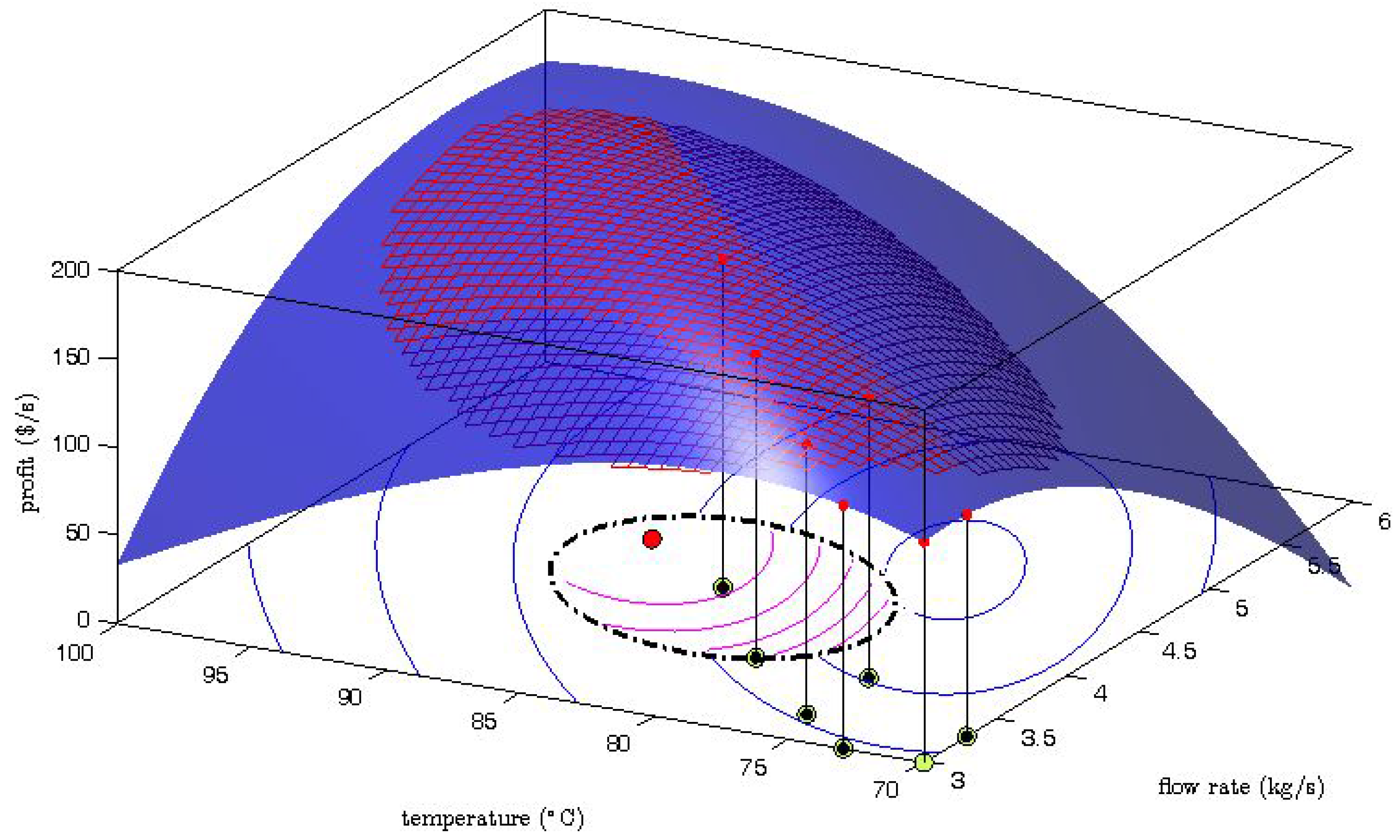
The generation of the explorative moves is presented in
Figure 2 where one MAWQA iteration for the optimization of the steady-state profit of the Williams-Otto reactor with respect to the flow rate and the reaction temperature [
6] is illustrated. Here the blue surface represents the real profit mapping, and the mesh represents the quadratic approximation which was computed based on the regression set (
![Processes 04 00045 i001]()
: set-point moves,
: measured profit values). The bottom part shows the contours of the profit as predicted by the uncorrected model (blue lines) , the constrained search space (dash-dot line), and the contours of the modifier-adapted profit (inside, magenta lines). Comparing the surface plot and the mesh plot, we can see that the gradient along the direction of the last set-point move is estimated well. However, a large error can be observed in the perpendicular direction. The gradient error propagates to the modifier-adapted contours and therefore, the next set-point move (
![Processes 04 00045 i003]()
) points to the direction where the gradient is badly estimated. Despite the fact that the move may not improve the objective function, the data collection in that direction can later help to improve the gradient estimation.
The example illustrates how the gradient error in a specific direction may lead to an explorative move along the same direction. In the MAWQA algorithm, the gradients are determined by evaluating
and
at
. In order to be able to quantify the gradient error, we assume that the screened set
is of size
and the quadratic approximations are interpolated based on
. In the application of the MAWQA algorithm, this assumption is valid when the current set-point is far away from the plant optimum. Recall the screening algorithm,
consists of the near set
and the distant set
. From (
4), we can conclude that the distant set
is always of size
. Step 4 of the MAWQA algorithm ensures that the near set
only consists of
until the optimized next move is such that
and there are no points
such that
, that is, all the points in
keep suitable distances away from
for good local approximations. The above two conditions imply that
, where
represents the plant optimum. As a result of Step 4, when
,
is always of size 1. For simplicity, a shift of coordinates to move
to the origin is performed and the points in
are reordered as
, where
.
Let
represent a natural basis of the quadratic approximation. Let
represent a column vector of the coefficients of the quadratic approximation. The quadratic approximation of the objective function is formulated as
where
. The coefficients
,
are calculated via the interpolation of the
data sets
where
,
, represent the polynomial bases in
,
and
ν represent the noise-free objective and the measurement noise. Assume
is nonsingular,
The computed gradient vector at the origin via the quadratic approximation is
where
represents the noise-free estimation and
represents the influence of the measurement noise. From [
8], a bound on the error between the noise-free estimation
and
can be obtained and simplified to
where
G is an upper bound on the third derivative of
, and Λ is a constant that depends on the distribution of the regression set
. Note that the bound in (
14) is defined for the error between the plant gradients and the estimated gradients. It is different from the lower and upper bounds on the gradient estimates which were studied by Bunin et al. [
5]. To simplify the study of Λ, assume
. Λ is defined as
where
,
, are the Lagrange polynomial functions that are defined by the matrix determinants
with the set
. The determinant of
is computed as
Let
represent the volume of the
n-dimensional convex hull spanned by the row vectors of the matrix in (
17), we have
Except the vertex at the origin, all the other vertices of the convex hull distribute on a
n-dimensional sphere with radius
.
reaches its maximal value when the vectors are orthogonal to each other. Let
and
represent any two row vectors of the matrix in (
17). The angle between them
Note that the angle
is different from the angle
between vectors
and
The relationship between
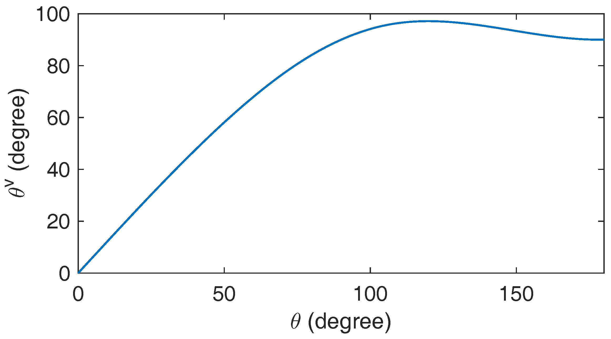
and
is illustrated in
Figure 3, where the angle between two 3-dimensional unit vectors is changed from 0 to 180 degree and the angle between the corresponding quadratic interpolation vectors increases proportionally when
degree and stays in an interval of [90 98] degree from 90 to 180 degree. Recall the screening for the distant set
via (
4), the consideration of the minimal angle at the denominator of the objective function ensures the choosing of the best set in terms of the orthogonality of the matrix in (
17) from all the collected data. As a result of (
14)–(
16) and (
18), the lowest bound of the error between
and
based on the collected data is achieved.
The error due to the measurement noise
can be calculated by Cramer’s rule
where
is the matrix formed by replacing the (
i + 1)th column of
by the column vector
,
is the level of the measurement noise,
, and
represents the scaled vector of noises. In order to reduce
, the value of
should be large enough. However, from (
14) the error bound will increase accordingly. The optimal tuning of
according to
and
G can be a future research direction. For a given distribution of
, the relative upper bound of
is related to the variance of the elements at the (
i + 1)th column. To show that, we start from the angle between the (
i + 1)th column vector and the first column vector
where we use
β to differentiate the angle from that formed by the row vectors. The variance of the elements at the (
i + 1)th column is
From (
22) and (
23), we obtain that
For the same mean value, the orthogonality of the (i + 1)th column vector to the first column vector can be quantified by the variance of the elements at the (i + 1)th column. As discussed before, the absolute value of the determinant of is influenced by the orthogonality. As a result, to replace a column of elements with small variance leads to a higher upper bound of the error than to replace a column of elements with large variance. Note that this is consistent with the constrained search space which is defined by the covariance matrix of the regression set.
From (
14) and (
21), three factors determine the gradient estimation errors
Distribution of the regression set (quantified by Λ and the distance to the current point)
Non-quadratic nature of the plant (quantified by G, the upper bound on the third derivative)
Measurement noise (quantified by ).
Figure 4 depicts how the three factors influence the generation of the explorative moves. Assume the plant functions are approximately quadratic in the region
around the current set-point and the value of
is large enough, a well-distributed regression set normally leads to a performance-improvement move. If the regression set is not well-distributed but the plant functions are approximately quadratic, a performance-improvement move is still possible if the level of the measurement noise
is low. This is illustrated in
Figure 5, where noise-free data was considered and the MAWQA algorithm did not perform any explorative moves. The explorative moves are only generated when either the plant functions deviate significantly from quadratic functions or the level of the measurement noise
is large. In the case shown in
Figure 2, the mapping of the plant profit is approximately quadratic but considerable measurement noise was presented. As a result, the unfavourable distribution of the regression set leads to an explorative move.
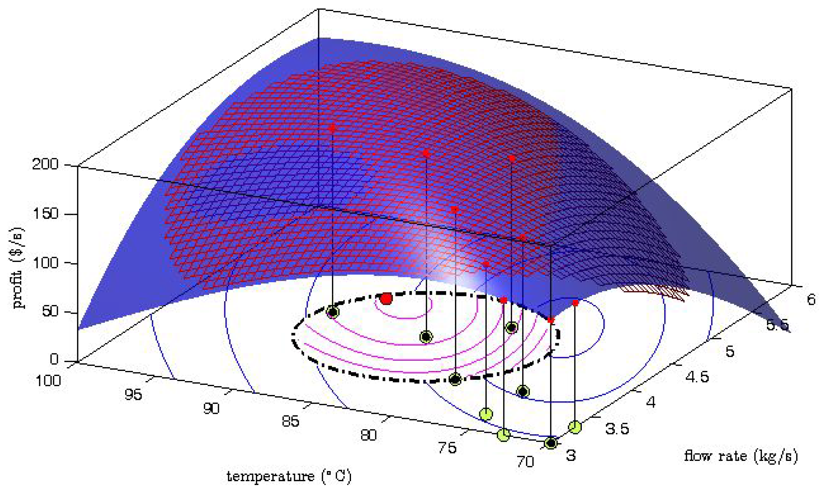
Gao et al. [
6] proved that the explorative moves can ensure an improvement of the accuracy of the gradient estimation in the following iterations. As an example,
Figure 6 shows the MAWQA iteration after two explorative moves for the optimization of the Williams-Otto reactor with noisy data [
6]. The mesh of the quadratic approximation well represents the real mapping (the blue surface) around the current point which locates at the center of the constrained search space (defined by the dash-dot line). The computed gradients based on the quadratic approximation are more accurate than those based on the quadratic approximation in
Figure 2. As a result, a performance-improvement move (represented by
![Processes 04 00045 i003]()
) was obtained.
4. Simulation Studies
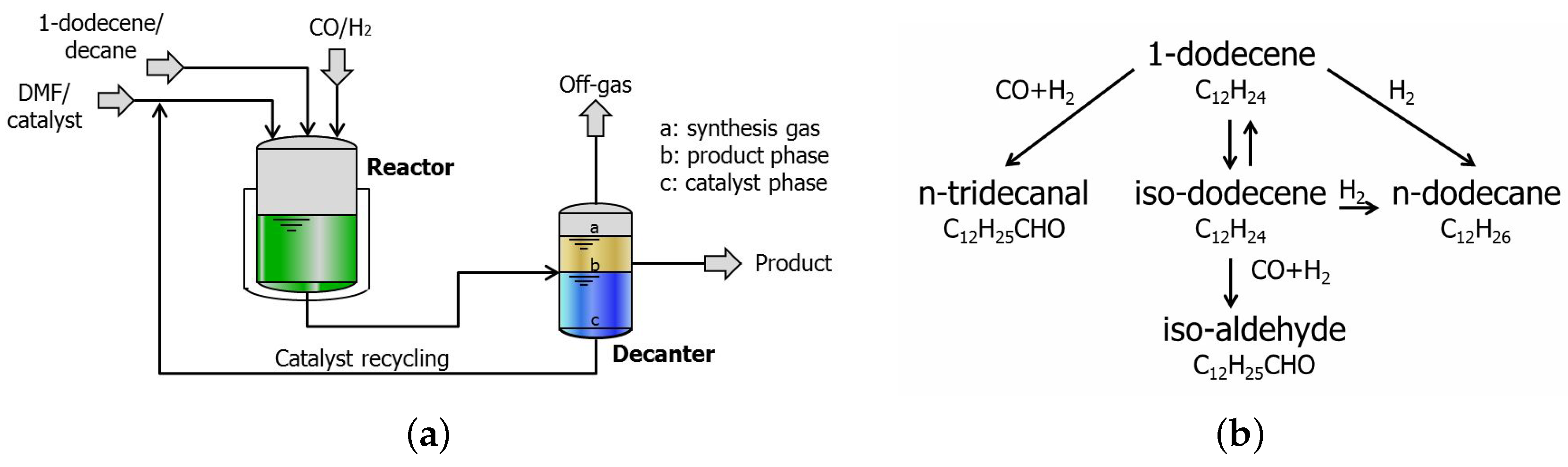
The optimization of a hydroformylation process with four optimization variables is used to illustrate the efficiency of the MAWQA algorithm over the finite difference based modifier adaptation algorithm. The continuous hydroformylation of 1-dodecene in a thermomorphic multicomponent solvent (in short TMS) system is considered. This process was developed in the context of the collaborative research centre InPROMPT at the universities of Berlin, Dortmund and Magdeburg and was demonstrated on miniplant scale at TU Dortmund [
9].
Figure 7 illustrates the simplified flow diagram of the TMS system together with the reaction network. The TMS system consists of two main sections: the reaction part and the separation part (here a decanter). The feed consists of the substrate 1-dodecene, the apolar solvent
n-decane, the polar solvent dimethylformamide (in short DMF), and synthesis gas (
). The catalyst system consists of
and the bidentate phosphite biphephos as ligand. During the reaction step, the system is single phase, thus homogeneous, so that no mass transport limitation occurs. During the separation step a lower temperature than that of the reactor is used and the system exhibits a miscibility gap and separates into two liquid phases, a polar and an apolar phase. The apolar phase contains the organic product which is purified in a down-stream process, while the catalyst mostly remains in the polar phase which is recycled. The main reaction is the catalyzed hydroformylation of the long-chain 1-dodecene to linear
n-tridecanal. Besides the main reaction, isomerization to iso-dodecene, hydrogenation to
n-dodecane and formation of the branched iso-aldehyde take place. Hernández and Engell [
10] adapted the model developed by Hentschel et al. [
11] to the TMS miniplant by considering the material balances of the above components as follows:
where (
25) is applied to the liquid components 1-dodecene,
n-tridecanal, iso-dodecene,
n-dodecane, iso-aldehyde, decane, and DMF. (
26) is applied to the gas components CO and
. The algebraic equations involved in the model are as follows:
Table 2 lists all the symbols used in the model together with their explanations. The optimization problem is formulated as the minimization of the raw material and operating cost per unit of n-tridecanal produced
where
and
represent the prices of 1-dodecene and of the catalyst,
and
are the molar flow rates,
and
are the operating costs of cooling and heating, and
is the molar flow rate of n-tridecanal, the vector of the optimization variables
consists of the reactor temperature, the catalyst dosage, the pressure and the composition of the synthesis gas. A sensitivity analysis was performed on the different model parameters and it was found that the gas solubility and the equilibrium constants for the catalyst species have the largest influence on the cost function. In our study of the MAWQA approach, the plant-model mismatch is created by decreasing the Henry coefficients
by
and ignoring the influence of CO on the active catalyst (
) in the model that is used by the optimization.
Table 3 lists the operating intervals of the optimization variables and compares the real optimum with the model optimum. In order to test the robustness of the approach to noisy data, the real cost data is assumed to be subject to a random error which is normally distributed with standard deviation
σ.
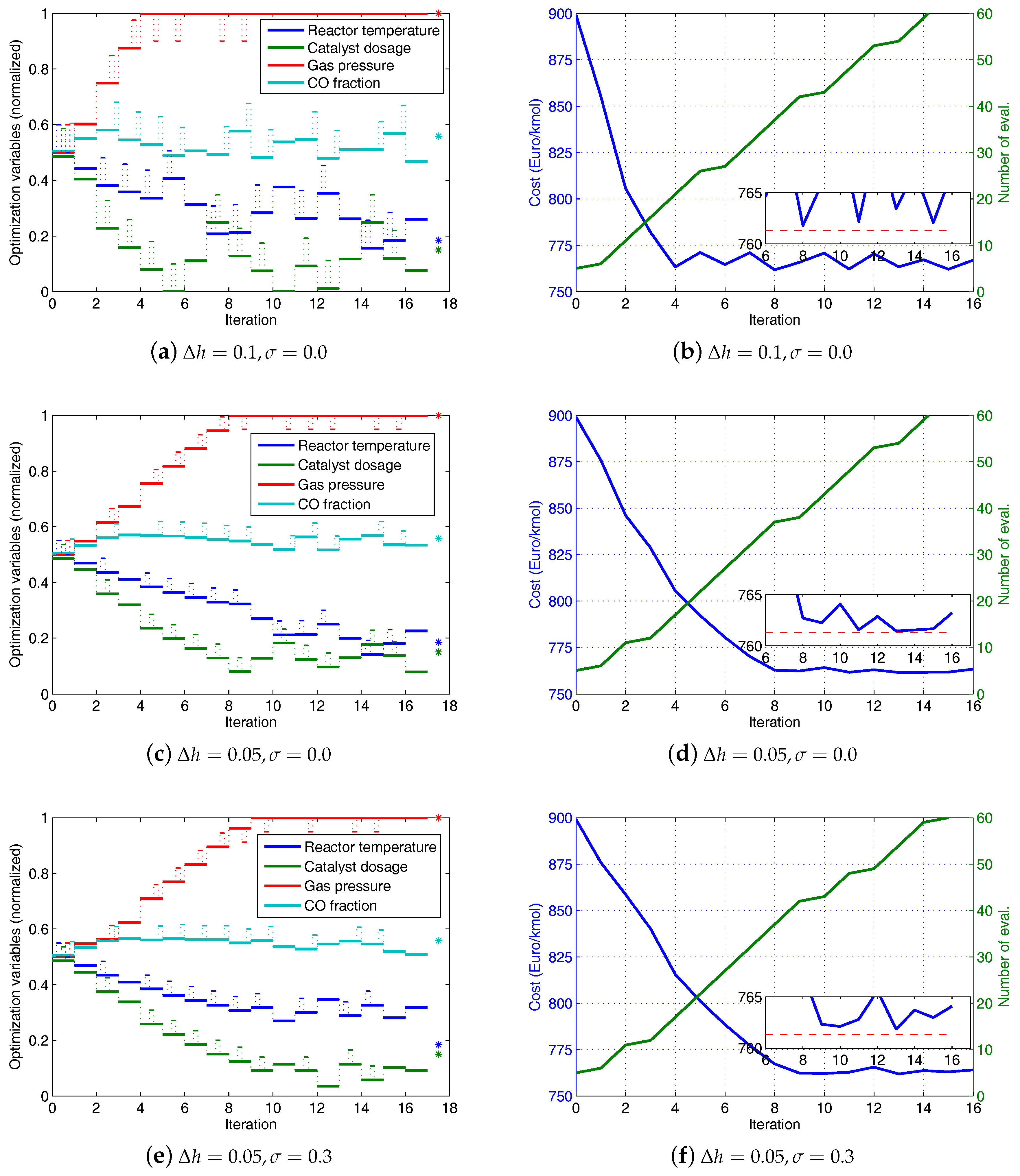
Simulation results of the modifier-adaptation approach using finite-difference approximation of gradient are illustrated in
Figure 8. The figures on the left show the evolutions of the normalized optimization variables with respect to the index of RTO iterations. The small pulses, which are superimposed on the evolutions, represent the additional perturbations required for the finite-difference approximations of the gradients. The star symbols at the right end mark the real optima. The figures on the right show the evolutions of the cost and the number of plant evaluations with respect to the index of the RTO iteration. The inset figure zooms in on the cost evolution, and the dashed line marks the real optimum of the cost. Three cases with different combinations of the step size of the perturbation and the noise in the data are considered. In the first case a large step-size,
, is used and the data is free of noise (
). From
Figure 8a we can see that three of the four optimization variables are still away from their real optimal values after 16 iterations. The cost evolution in
Figure 8b shows an oscillating behavior above the cost optimum. This indicates that the step-size is too large to enable an accurate estimation of the gradients.
In the second case a reduced step-size (
) is tried. From
Figure 8c we can see that the optimization variables attain their real optimal values at the 14th iteration. However, numerical errors of the simulation of the plant cause deviations during the following iterations. On the one hand, the use of a small step-size reduces the error of the finite-difference approximation of the gradients. On the other hand, the small step-size leads to a high sensitivity of the gradient approximation to errors. This is illustrated by the third case, in which the data contains a normally distributed error (
). The optimization variables do not reach the real optima (see
Figure 8e,f).
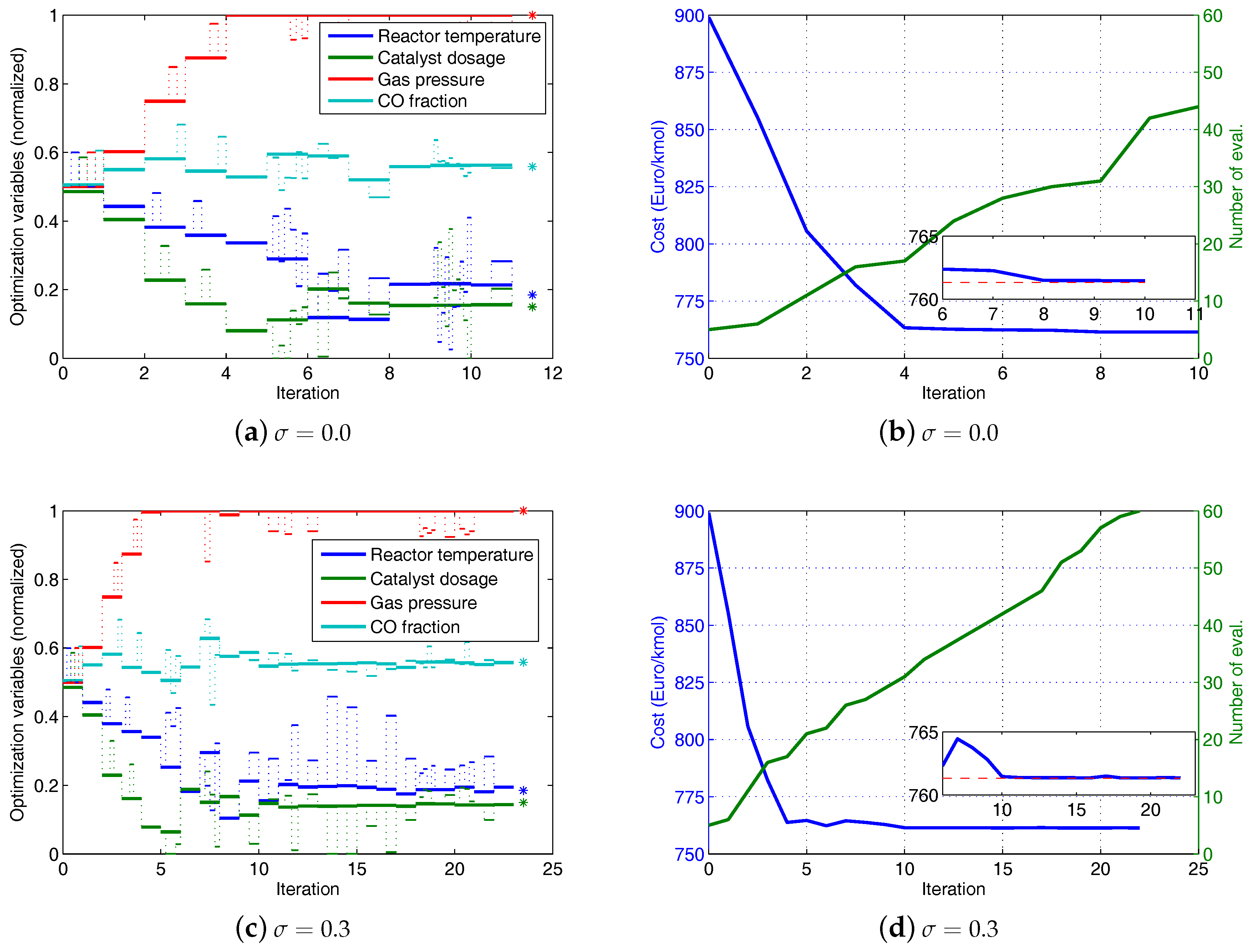
Simulation results of the MAWQA algorithm are illustrated in
Figure 9. The parameters of the MAWQA algorithm are listed in
Table 4. The figures on the left show the evolutions of the normalized optimization variables with respect to iteration. The small pulses, which are superimposed on the evolutions, represent the additional plant evaluations, i.e., initial probes and explorative moves. The real optima are marked by the star symbols. The figures on the right show the evolutions of the cost and the number of plant evaluations with respect to the iterations. The inset figure zooms in on the cost evolution, and the dashed line marks the real optimum of the cost. In the first 4 iterations, the modifier-adaptation approach using finite-difference approximation of gradient is run. Afterwards, enough sampled points (here
) are available for the quadratic approximation and the MAWQA approach is run. In the case of noise-free data, the MAWQA approach takes 8 iterations to reach the real optima approximately (see
Figure 9a). The total number of plant evaluations is 30, much less than that used in the second case of the finite-difference approximations of gradients which requires 55 plant evaluations to reach a similar accuracy. Note that the additional plant evaluations at the 10th iteration are attributed to the shrinking of the regression region by Step 4 of the MAWQA algorithm.
Figure 9c,d show the optimization results in the presence of noise. The MAWQA algorithm takes 10 iterations to reach the real optima.
Finally, the MAWQA algorithm was tested with different values of the parameters. For each parameter, three values are considered and the costs after 30 plant evaluations are compared with the real optimum. The results are summarized in
Table 5. The increase of
leads to a decrease of the accuracy of the computed optima. This is due to the fact that the true mapping is only locally quadratic and therefore the use of too distant points can cause large approximation errors. The value of
γ influences the rate of convergence since it is directly related to the size of the search space in each iteration. The value of
determines the accuracy of the finite-difference approximation of the gradients at the starting stage of the MAWQA approach. In the absence of noise, a small
is preferred. However, the search space is also determined by the distribution of the sampled points. A small
leads to a more constrained search space and therefore decreases the rate of convergence. The overall influence of
on the rate of convergence is a combination of both effects. Note that
does not influence the accuracy of the optima if enough plant evaluations are performed.


 : set-point moves, : measured profit values). The bottom part shows the contours of the profit as predicted by the uncorrected model (blue lines) , the constrained search space (dash-dot line), and the contours of the modifier-adapted profit (inside, magenta lines). Comparing the surface plot and the mesh plot, we can see that the gradient along the direction of the last set-point move is estimated well. However, a large error can be observed in the perpendicular direction. The gradient error propagates to the modifier-adapted contours and therefore, the next set-point move (
  ) points to the direction where the gradient is badly estimated. Despite the fact that the move may not improve the objective function, the data collection in that direction can later help to improve the gradient estimation.
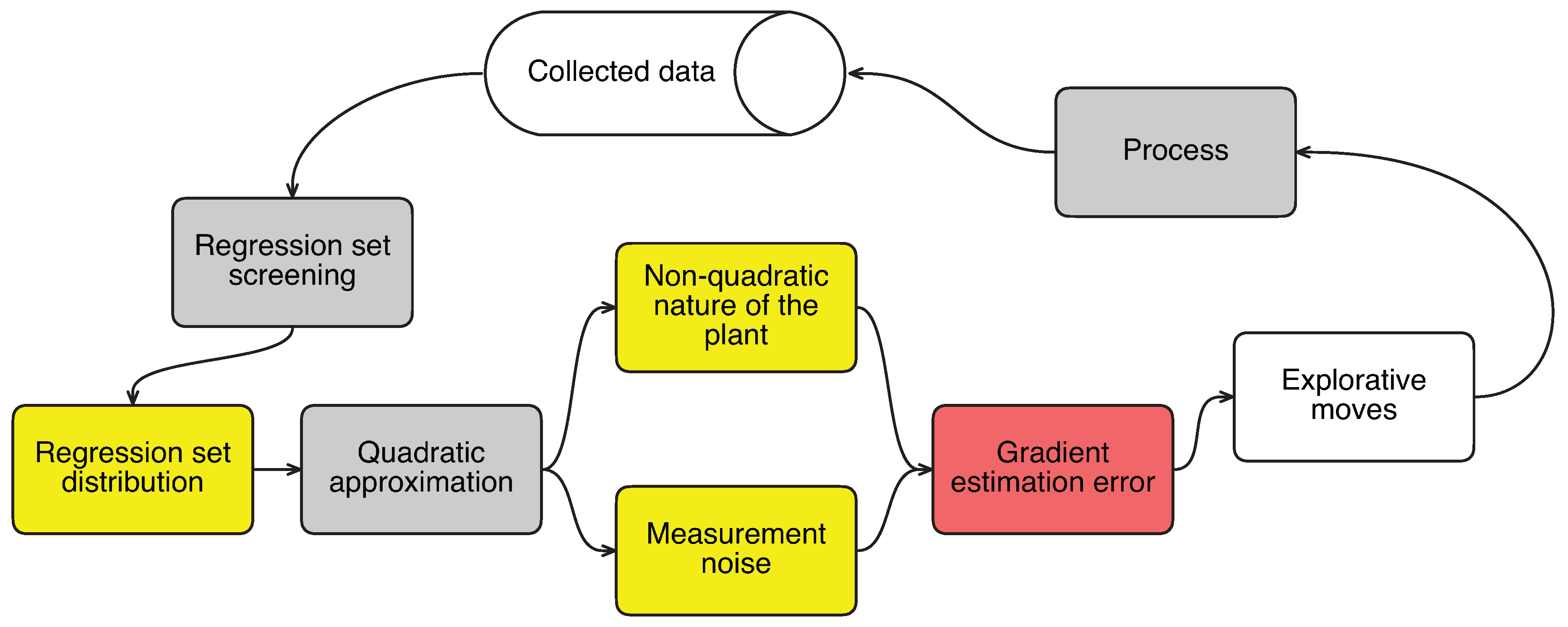
 : not chosen set-point, : measured profit,
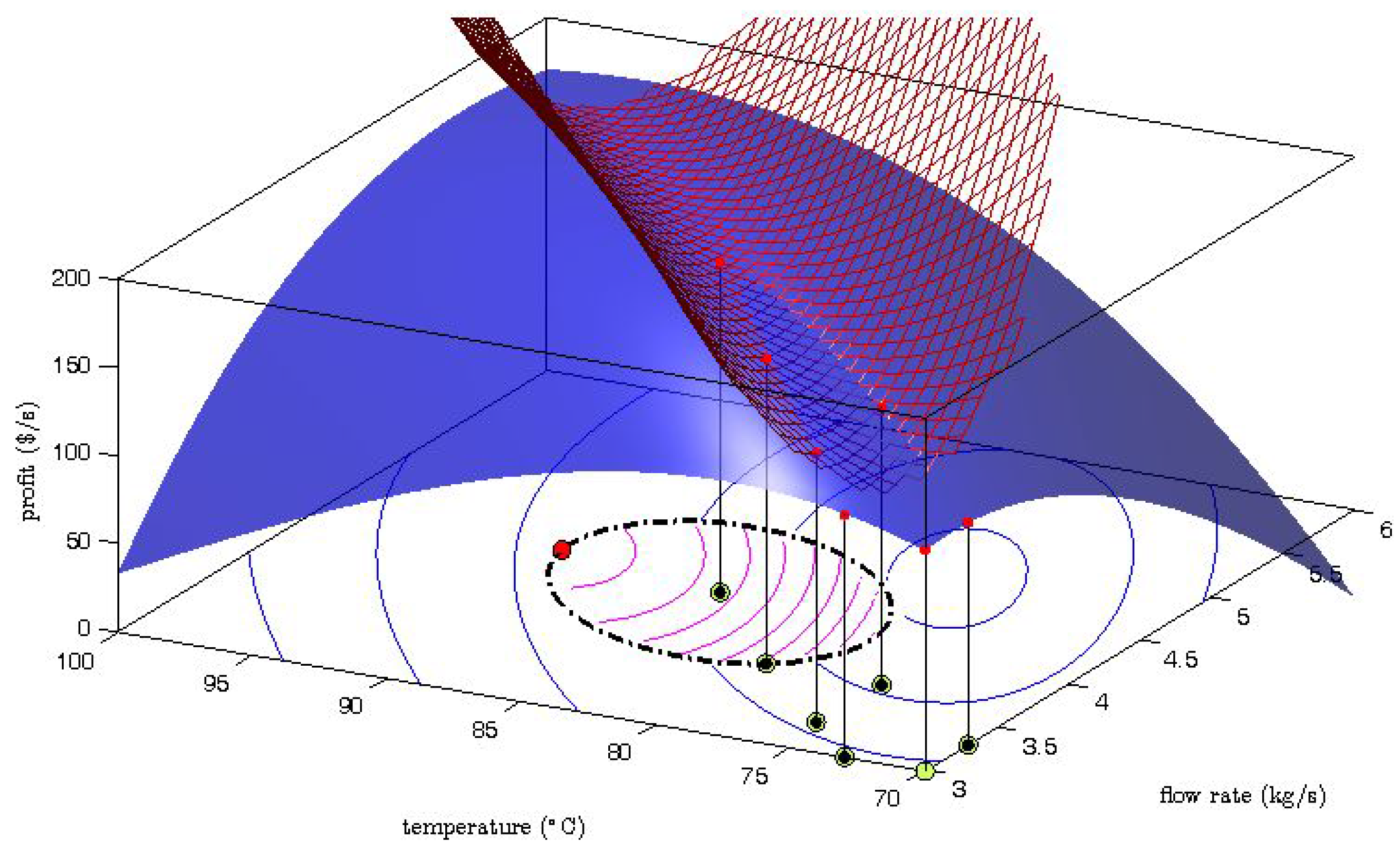
