
Dynamic Optimization in JModelica.org †

1
Department of Automatic Control, Lund University, SE-221 00 Lund, Sweden
2
Modelon AB, Ideon Science Park, SE-223 70 Lund, Sweden
*
Author to whom correspondence should be addressed.
†
This paper is an extended version of our paper published in Proceedings of the 9th International Modelica Conference, Munich, Germany, 3–5 September 2012, Collocation Methods for Optimization in a Modelica Environment.
Processes 2015, 3(2), 471-496; https://doi.org/10.3390/pr3020471
Submission received: 13 April 2015
/
Revised: 30 May 2015
/
Accepted: 10 June 2015
/
Published: 19 June 2015
(This article belongs to the Special Issue Algorithms and Applications in Dynamic Optimization)
Abstract
:We present the open-source software framework in JModelica.org for numerically solving large-scale dynamic optimization problems. The framework solves problems whose dynamic systems are described in Modelica, an open modeling language supported by several different tools. The framework implements a numerical method based on direct local collocation, of which the details are presented. The implementation uses the open-source third-party software package CasADi to construct the nonlinear program in order to efficiently obtain derivative information using algorithmic differentiation. The framework is interfaced with the numerical optimizers IPOPT and WORHP for finding local optima of the optimization problem after discretization. We provide an illustrative example based on the Van der Pol oscillator of how the framework is used. We also present results for an industrially relevant problem regarding optimal control of a distillation column.
1. Introduction
The application of optimization to large-scale dynamic systems has become more common in both industry and academia during the last decades. Dynamic Optimization Problems (DOP) occur in many different fields and contexts, including optimal control, parameter and state estimation, and design optimization. Examples of applications are minimization of material and energy consumption during set point transitions in power plants [1] and chemical processes [2], controlling kites for wind power generation [3], and estimating occupancy and ambient air flow in buildings [4].
The applications are diverse and occur in both online and offline settings. Online optimal control is usually done in the form of Model Predictive Control (MPC) and online state estimation based on dynamic optimization is usually done in the form of Moving Horizon Estimation (MHE) [5]. Offline applications include finding optimal trajectories, which can be used either as a reference during manual control or as reference trajectories combined with online feedback to handle deviations due to model uncertainty and disturbances.
JModelica.org [6,7] is a tool targeting model-based analysis of large-scale dynamic systems, in particular dynamic optimization. It uses the modeling language Modelica [8] to describe system dynamics, and the optimization formulation is done with the use of the Modelica language extension Optimica [9]. Unlike most other tools for dynamic optimization, the use of Modelica allows the user to create their dynamic system models using a dedicated and modern modeling language, instead of relying on standard imperative programming languages that are ill-suited for advanced system modeling. It also makes the model implementation tool-independent, since there are a wide range of tools that support the Modelica language.
This paper presents the newest generation of algorithms in JModelica.org for solving DOPs and the surrounding framework. The toolchain starts with the JModelica.org compiler, which processes the Modelica and Optimica code and performs symbolic transformations. The compiler then creates a symbolic representation of the DOP using CasADi (see Section 3.3.1). This representation is used to transcribe the problem into a nonlinear program (NLP) using direct local collocation. Finally, the NLP is solved using IPOPT [10] or WORHP [11]. The needed first- and second-order derivatives are provided by CasADi’s algorithmic differentiation.
The outline of the paper is as follows. Section 2 presents the class of problems that the framework aims to solve and common methods for treating this kind of problem. Section 3 presents other available tools that target the same kind of problem, and also the software and languages used to implement the framework in JModelica.org. Section 4 provides the details of how the framework discretizes the infinite-dimensional optimization problem using direct collocation. Section 5 discusses considerations that are needed to employ direct collocation in practice and also additional features available in the framework. Section 6 presents the implementation of the framework. Section 7 presents an example on how to solve a simple optimal control problem based on the Van der Pol oscillator using the framework. It also presents results obtained for an industrially relevant example of control of a distillation column. Finally, Section 8 summarizes the paper and discusses future work.
Regarding notation, scalars and scalar-valued functions are denoted by regular italic letters x. Vectors and vector-valued functions are denoted by bold italic letters x, and component k of x is denoted by xk. The integer interval from a ∈ ℤ to b ∈ ℤ (inclusive) is denoted by [a..b].
2. Dynamic Optimization
In this section, we will give a description of the class of problems that the framework aims to solve. We consider optimization problems that involve a dynamic system with some degrees of freedom, typically time-varying control signals or time-invariant parameters. These problems are typically infinite-dimensional and their numerical solution consequently involves a discretization of the system dynamics. We restrict ourselves to problems with finite (but not necessarily fixed) time horizons and systems described by differential-algebraic equation (DAE) systems. We also provide an overview of the most widely used methods for numerically solving DOPs.
2.1. Problem Formulation
We consider systems whose dynamics are described by an implicit DAE system. Specifically, we consider DAE systems of the form
where t ∈ [t0, tf] is the sole independent variable: time,
is the differential variable,
is the algebraic variable,
is the control variable, and
is the vector of parameters to be optimized—that is, the free parameters. For now we also assume that the DAE system is of most index one, meaning that the Jacobian of F is nonsingular with respect to
and y. We will comment on the treatment of high-index DAE systems in Section 3.3.2.
Initial conditions are also given on an implicit form; that is,
For ease of notation, we compose the time-dependent variables into a single variable z; that is,
where nz := 2 · nx + ny + nu. The system dynamics are thus fully described by
where
The initial conditions are assumed to be consistent with the DAE system, meaning that they provide sufficient information to solve for the initial state. The domains of F and F0 can be further restricted by the introduction of variable bounds, as discussed below. We do not consider systems that have integer variables or time delays.
The problem considered throughout the paper is to
We will now discuss the concepts and notation used in Equation (2). The time horizon endpoints t0 and tf may be either free or fixed. Equation (1) has been introduced as a constraint in Equation (2b). Consequently, the optimization variables are not only those generating degrees of freedom (u, p, t0, and tf), but also the system variables x (which inherently determines
) and y. Note that solving the initial equations for the initial state will be done as a part of solving the optimization problem, which for example enables the treatment of problems where the initial state is unknown.
Equation (2a) is the objective and is a Bolza functional—as is typical for optimal control problems ([12] Section 3.3) but general enough to cover other problems of interest, such as parameter estimation—where ϕ is called the Mayer term and L is called the Lagrange integrand. A more standard form for the Mayer term would be ϕ(tf, z(tf), p), but here we work with a generalized form. The essence of the generalization is that instead of depending on only the terminal state, it depends on the state at a finite, arbitrary number of time points within the time horizon. This gives rise to the notion of timed variables, which we denote by zT, which we define by first denoting the needed time points by T1,
, where nT ∈ Z is the number of such time points. These time points must be equal to a convex combination of t0 and tf; that is, for all j there must exist a fixed θj ∈ [0, 1] such that Tj = (1 − θj)t0 + θjtf. For problems with a fixed time horizon, this simply means that Ti ∈ [t0, tf]. For problems with a free time horizon, this means that the location of the time points depend on the optimal t0 and tf. We then let
The standard Mayer term only involves the single time point T1 = tf. One application of the generalized Mayer term is the formulation of parameter estimation problems, where there typically is measurement data for the system outputs at discrete time points, which is used to penalize the deviation of the model output from the data values at these points. An alternative approach in this case is to interpolate the measurement data to form a continuous-time measurement trajectory. This trajectory can then instead be used to form a Lagrange integrand which penalizes the deviation of the model output from the measurements. The occurrence of the timed variables zT is not restricted to the Mayer term. The timed variables can also be used in the Lagrange integrand and the constraints, as discussed below. A more common (and also more general) approach to treating timed variables is by introducing multiple phases ([13] Section 3.7), which we do not consider further in this paper.
Equation (2c) is variable bounds, which are enforced during the entire time horizon [t0, tf], where
and
are the lower bounds and
and
are the upper bounds. The constraints Equation (2d) are path constraints, which are generalizations of the variable bounds. They are separated from the variable bounds, since the bounds can be treated more efficiently by many numerical algorithms. For example, an interior-point algorithm will ensure that the bounds are satisfied even during iteration, thus restricting the domains of the NLP functions. Finally, Equation (2e) is point constraints. These are similar to the path constraints, with the difference being that they are only enforced at specific time points, rather than during the entire time horizon. The time points Tj that were used to generalize the Mayer term are also used to formulate the point constraints. The path constraints may also depend on the timed variables. The number of time points nT is thus not only the number of time points involved in the Mayer term, but also includes the number of time points needed to formulate the Lagrange term as well as the path and point constraints.
The objective functions ϕ and L, the DAE system and initial condition residuals F and F0, the path constraint functions ge and gi as well as the point constraint functions Ge and Gi must all be twice continuously differentiable with respect to the arguments that correspond to any of DOP variables. For example, F must be twice continuously differentiable with respect to its second argument, corresponding to the system variables z, but not with respect to its first argument, corresponding to the explicit time dependence. These continuity requirements are needed to apply techniques based on Newton’s method to find a solution to first-order optimality conditions. Equation (2c)–(2e) are optional, whereas Equations (2a) and (2b) are necessary to get a sensible DOP (although Equation (2a) can be removed to obtain a feasibility problem). No assumptions of linearity or convexity are made. The problem will thus in general be nonconvex and we will not endeavor to find a global optimum. We will instead use first-order necessary optimality conditions to find a local optimum.
2.2. Numerical Methods
There are many approaches to numerically solving DOPs, which stem from the theory of optimal control. The earliest methods date back to the 1950s and are based on Bellman’s dynamic programming, of which a modern description can be found in for example [14]. The main result on dynamic programming for continuous-time systems is the Hamilton-Jacobi-Bellman equation, which is a nonlinear partial differential equation. The dynamic programming framework is theoretically appealing, due to providing sufficient conditions for global optimality and state feedback laws. However, in practice it suffers from the curse of dimensionality: The dimension of the partial differential equation increases with the dimension of the system state. Numerical methods based on dynamic programming are thus only computationally tractable for small-scale problems.
The most widely used numerical techniques for optimal control today are instead based on first-order necessary conditions for local optimality. Surveys of these are available in for example [15,16] and an overview is illustrated in Figure 1. They can be categorized according to their respective answers to two questions; when to discretize the system dynamics corresponding to Equation (1), and how to discretize them? There are essentially two answers to the first question, which have lead to the two categories of indirect and direct methods. Indirect methods start by establishing the optimality conditions, and then discretize the resulting differential equations to find a numerical solution. Direct methods instead first discretize the dynamics and then establish the optimality conditions. Indirect methods are based on calculus of variations and Pontryagin’s maximum principle, which provide optimality conditions in the form of boundary value problems. Standard numerical methods for boundary value problems can then be employed to solve the problem numerically. Direct methods instead reduce the DOP to an NLP by discretization. The optimality conditions are then given by the Karush-Kuhn-Tucker (KKT) conditions.
Both direct and indirect approaches discretize differential equations, and the same discretization methods are commonly used for both approaches. The most common methods belong to one of two families: shooting and collocation. The simplest form of shooting is single shooting, which parametrizes the control—explicitly for the direct method and implicitly by the maximum principle and costate initial values for the indirect method—and then numerically integrates to tf and iteratively updates the control based on sensitivities. The numerical robustness of single shooting can be improved by dividing the time horizon into subintervals. Single shooting is then applied within each subinterval, by introducing the subinterval boundary values as variables and imposing linking constraints between the subintervals. This is called multiple shooting, which essentially decouple the dynamics between the subintervals.
The second family of discretization methods is collocation. These methods simultaneously discretize the differential equations over the entire time horizon using implicit Runge-Kutta methods. Consequently, they do not rely on external numerical integrators, because after the full discretization of the differential equations the optimality conditions are reduced to an algebraic root finding problem. Collocation methods can be either local, where the time horizon is divided into elements and low-order polynomials are used to approximate the trajectories within each element, or global, where a single high-order polynomial is used over the entire time horizon.
Shooting methods (especially single shooting) lead to optimization problems with few variables but highly nonlinear functions—due to their internalization of the differential equations and numerical integrators—whereas simultaneous methods lead to problems with less severe nonlinearities but many variables. Indirect methods need good initial guesses of the costates and also identification of the switching structure of inequality constraints, both of which require proficiency in the maximum principle for all but the most simple problems. Single shooting suffers from the numerical sensitivity discussed above. Thus, direct multiple shooting and direct collocation appear to be the most suitable methods to be used in a high-level framework for large-scale dynamic optimization. JModelica.org uses a method based on direct collocation, which is presented in Section 4.
3. Related Software and Languages
In this section we first give an overview of modern tools that are available for dynamic optimization. We then discuss the software and languages used in the dynamic optimization framework in JModelica.org.
3.1. Tools for Dynamic Optimization
One approach to solving Equation (2) numerically is to manually discretize the dynamics and then encode the discretized problem in an algebraic modeling language for optimization. Mature examples of such are AMPL [17] and GAMS [18], whereas Pyomo [19] is a modern example. A more convenient approach is to use a tool tailored for dynamic optimization in which the DOP can be formulated in its natural, undiscretized form. The tool then handles the details of the discretization. An important dichotomy of such tools is whether they use existing general-purpose programming languages, such as MATLAB or C++, or dedicated modeling languages to describe the system dynamics. Some noteworthy examples of modern dynamic optimization tools of the former category are ACADO Toolkit [20] and PROPT [21]. ACADO Toolkit is an open-source, self-contained C++ package for dynamic optimization. It primarily uses direct multiple shooting and is designed for implementation of online MPC or MHE on embedded hardware. PROPT is a commercial package for MATLAB based on TOMLAB [22] using direct global collocation. It supports a wide range of optimization problems, including problems with multiple phases and integer variables.
Component-based modeling of large-scale, complex dynamical systems benefits greatly from the expressiveness offered by dedicated dynamic modeling languages. It also decouples the modeling process from the computational aspects, allowing the same model implementation to be used for multiple purposes, such as simulation and optimal control. Examples of modern dynamic optimization tools that utilize a dedicated language for modeling are APMonitor [23], gPROMS [24], and JModelica.org [6]. APMonitor is freely available and uses its own modeling language and direct local collocation. It has a tight and user-friendly integration between simulation, estimation, and control of dynamic systems, both dynamically and in steady state. It offers interfaces to Python, MATLAB and web browsers. gPROMS is a large family of commercial products for model-based chemical engineering, which are based on gPROMS’s powerful object-oriented modeling language. While not its primary focus, it has capabilities for dynamic optimization using shooting algorithms.
3.2. Modelica and Optimica
JModelica.org uses Modelica [8] to describe the dynamic system model. Modelica is an object-oriented language targeting modeling of heterogeneous physical systems. It is based on a declarative equation-based paradigm designed for both textual and graphical modeling. Accordingly, there is no need to manually solve the equations for the derivatives, which is common in block-based modeling formalisms. Modular modeling is extensively supported by defining acausal physical ports for elementary components, building systems by hierarchical aggregation of subsystems, and managing model variants by replacing some parts of the model by others that share the same physical interface.
Modelica is a non-proprietary language supported by several tools. It features an open standard library of physical components in a wide range of engineering domains, including thermodynamics, mechanics, electronics, and control. There is also a large number of other model libraries available, both freely and commercially, developed by academia and industry.
Modelica is designed mainly with simulation-based analysis in mind, and thus lacks native support for optimization formulations. To accommodate the need for formulation of DOPs based on Modelica code, the language extension Optimica [9] was developed and integrated with JModelica.org. Optimica defines new syntax and semantics for specifying constraints and an objective. Optimica was previously used only in JModelica.org but has since also been adopted by OpenModelica [25] to solve optimal control problems described in Modelica using direct multiple shooting or collocation. Optimica also served as a basis for IDOS [26], an online environment for solving a wide variety of optimal control problems using different techniques. Optimization has started to gain traction within the Modelica community and there are ongoing efforts within MODRIO [27] to standardize DOP formulations based on Modelica.
Modelica is used in the presented framework for two main reasons: First, it gives the user access to a powerful modeling language, which is important for large-scale, component-based system modeling. Second, it allows existing Modelica models to be reused for dynamic optimization. However, since typical Modelica models are intended for high-fidelity simulation, they are often too complex in terms of size or lack of differentiability for optimization purposes out-of-the-box.
3.3. Software Used to Implement Framework
JModelica.org integrates many different software packages. In this section, we present the most important ones, especially those that are prominent in the dynamic optimization framework.
3.3.1. CasADi
To solve Equation (2), we will employ direct local collocation to transcribe the problem into an NLP. A local optimum to the NLP will be found by solving the first-order KKT conditions, using iterative techniques based on Newton’s method. This requires first- and second-order derivatives of the NLP cost and constraint functions with respect to the NLP variables. The framework uses CasADi to obtain these.
CasADi [28] (Computer algebra system with Automatic Differentaion) is a low-level tool for efficiently computing derivatives using AD and is tailored for dynamic optimization. Once a symbolic representation of an NLP has been created using CasADi primitives, the needed derivatives are efficiently and conveniently obtained and sparsity patterns are preserved. CasADi also offers interfaces to numerical optimization solvers, allowing for seamless integration with for example IPOPT and WORHP.
CasADi utilizes two different graph representations for symbolic expressions. The first is a scalar representation, called SX, where all atomic operations are scalar-valued, as is typical for AD tools. The second is a sparse matrix representation, MX, where all atomic operations instead are multiple-input, multiple-output, and matrix-valued. The MX representation is more general and allows for efficient—especially in terms of memory—representation of high-level operations, such as matrix multiplication and function calls. On the other hand, the SX representation offers faster computations by reducing overhead and performing additional symbolical simplifications.
A prototypical integration between CasADi and JModelica.org was first initiated in [29] and further developed in [30]. Previously, the integration relied on the JModelica.org compiler generating XML code symbolically describing the DOP. The XML code was then imported by CasADi and used to create a symbolic representation using CasADi primitives. The integration between JModelica.org and CasADi has since been redesigned and is now handled by CasADi Interface, as described below.
3.3.2. The JModelica.org Compiler
The JModelica.org compiler [31] is implemented in the compiler construction framework JastAdd [32]. JastAdd is an extension to Java and focuses on modular extensible compiler construction by aspect orientation. The compiler process is illustrated in Figure 2. The compiler first creates an internal representation of the Modelica and Optimica code in the form of an abstract syntax tree (AST). The AST is then used to perform standard compiler operations such as name and type analysis, but also Modelica-specific operations as described below.
Modelica is intended for object-oriented component-based modeling, resulting in hierarchical models. To get a representation of the model that is closer to a DAE system, one of the first steps, called flattening, is to resolve the class inheritance and instantiation in the model to arrive at a flat representation of the model. The flat representation essentially consists of only variable declarations and equations. Before the DAE system is interfaced with a numerical solver, various symbolic transformations are performed on it, such as alias elimination and index reduction. Component-based modeling often gives rise to many equations of the form x = ±y due to conservation laws, which are trivial to solve analytically. This process is called alias elimination. For DAE systems of index greater than 1, index reduction is performed using the dummy derivative method [33]. This allows for the treatment of high-index systems within the framework without having to worry about the numerical challenges that they often pose, such as drift or method order reduction.
Once all the symbolic transformations have been performed on the DAE system, it is coupled with the DOP formulation in the Optimica code. Note that although index reduction is performed on the DAE system, high-index path constraints Equation (2d) and bounds Equation (2c) are not index reduced by the compiler. The AST is then used to transfer the optimization problem to CasADi Interface by creating CasADi objects.
CasADi Interface [34] is a C++ package that enables the symbolic creation of DOPs using CasADi. It serves as an interface between DOPs formulated using Modelica and Optimica and the optimization algorithms that can be used to solve them. When using CasADi Interface, the JModelica.org compiler creates CasADi expressions for the DOP, effectively mapping the Modelica and Optimica languages onto CasADi constructs, which then can be used to obtain the derivative information that is typically needed by numerical optimizers. While CasADi Interface is designed with Modelica and Optimica in mind, there is nothing in it that is inherently dependent on these languages. It could thus potentially serve as an interface to other modeling languages as well.
3.3.3. Nonlinear Programming and Linear Solvers
To numerically solve the NLP arising from applying direct local collocation to Equation (2), JModelica.org uses third-party solvers. JModelica.org supports the use of IPOPT [10] and WORHP [11], through CasADi’s NLP solver interface. IPOPT is a primal-dual interior-point method and WORHP is an active set sequential quadratic programming method utilizing an interior-point method to solve the intermediate quadratic programs. Both solvers are designed for large-scale and sparse nonlinear programs. IPOPT is open source, whereas WORHP is commercial but offers free academic licenses. Both solvers need to solve a linear equation system in each iteration and utilize external sparse linear solvers for this purpose. Both IPOPT and WORHP have interfaces to the open-source linear solver MUMPS, and also the commercial HSL library [35], which offers free academic licenses, among others.
4. Direct Local Collocation
In this section, we formulate the mathematical description for the discretization procedure that is used to solve Equation (2) and implemented in the framework. The discretization is based on local direct collocation as described in [13,36]. The fundamental idea is to discretize the differential equations using finite differences, thus transforming the infinite-dimensional DOP into a finite-dimensional NLP. The discretization scheme is based on collocation methods, which are special cases of implicit Runge-Kutta methods and are also commonly used for numerical solution of DAE and stiff ODE systems [37].
4.1. Collocation Polynomials
The optimization time horizon is divided into ne elements. Let hi denote the length of element i, which has been normalized so that the sum of all element lengths is one. This normalization facilitates the solution of problems with free endpoints by keeping the normalized element lengths constant and instead varying t0 and tf. The time is normalized in element i according to
where τ is the normalized time,
is the corresponding unnormalized time, and ti is the mesh point (right boundary) of element i. This normalization enables a treatment of the below interpolation conditions that is homogeneous across elements.
Within element i the time-dependent system variable z is approximated using a polynomial in the local time τ denoted by
which is called the collocation polynomial for that element. The collocation polynomials are formed by choosing nc collocation points, which in this work are restricted to be the same for all elements. We use Lagrange interpolation polynomials to represent the collocation polynomials, using the collocation points as interpolation points. Let τk ∈ [0, 1] denote collocation point k ∈ [1..nc], and let
denote the value of zi(τk).
Since the differential variable x needs to be continuous on [t0, tf], we introduce an additional interpolation point at the start of each element for the corresponding collocation polynomials, denoted by τ0 := 0. We thus get the collocation polynomials
where
and ℓk are the Lagrange basis polynomials, respectively with and without the additional interpolation point τ0. The basis polynomials are defined as
Note that the basis polynomials are the same for all elements, due to the normalized time. These basis polynomials satisfy
The collocation polynomials are thus parametrized by the values zi,k = zi(τk).
In order to obtain the collocation polynomial for the differential variable derivative
in element i, the collocation polynomial xi is differentiated with respect to time. Using Equations (4) and (5), and the chain rule, we obtain
There are different schemes for choosing the collocation points τk, with different numerical properties, in particular regarding stability and order of convergence. The most common ones are called Gauss, Radau and Lobatto collocation [37]. The framework in JModelica.org has support for Radau and Gauss points. For the sake of brevity, we will in the next subsection present a transcription based on Radau collocation. The Radau collocation scheme always places a collocation point at the end of each element, and the rest are chosen in a manner that maximizes numerical accuracy.
4.2. Transcription of the Dynamic Optimization Problem
In this section Equation (2) is transcribed into an NLP, using the collocation polynomials constructed above. The optimization domain of functions on [t0, tf], which is infinite-dimensional, is thus reduced to a domain of finite dimension by approximating the trajectory z by a piecewise polynomial function.
As decision variables in the NLP we choose the system variable values in the collocation points, zi,k, the differential variable values at the start of each element, xi,0, the free parameters, p, the initial condition values, z1,0 := z(t0), and t0 and tf if they are free. We thus let
be the vector containing all the NLP variables, where
Note that the actual order of the variables in the implemented framework is different to allow contiguous access for efficiency reasons ([38] Section 5.2.2). With Radau collocation and the above choice of optimization variables, the transcription of Equation (2) results in the NLP
where
denotes the unnormalized collocation point k in element i. The rest of the concepts and notation used in Equation (7) will be discussed below.
There are two approaches in the treatment of the timed variables zT during the transcription. The first is to approximate z(Tj) by the value of its corresponding collocation polynomial, that is, zi(τ(Tj)). A less general approach is to assume that every time point Tj coincides with some collocation point ti,k; that is, there exists a map Γ : [1..nT] → [1..ne] × [1..nc] such that Tj = tΓ(j). We can then proceed to transcribe zT, defined by Equation (3), into
The former approach is more general, as it does not assume the existence of Γ. It is also more user-friendly, since it does not force the user to align the element mesh with the time points Tj. On the other hand, the latter approach is more efficient for large nT, which is typical for parameter estimation problems. The two approaches also have distinct numerical properties, which are outside the scope of this paper to analyze. Henceforth we adopt the latter approach, which assumes the existence of Γ.
Due to the assumed existence of Γ, the Mayer term of the Bolza functional is straightforward to transcribe as
where
denotes that b, which belongs to Equation (7), is the corresponding transcription of a, which belongs to Equation (2). The transcription of the Lagrange term is more involved and utilizes Gauss-Radau quadrature within each element:
where the quadrature weights ωk are given by
Equation (2a) is thus transcribed into Equation (7a).
The essence of direct collocation is in the transcription of the system dynamics in Equation (2b). Instead of enforcing the DAE system for all times t ∈ [t0, tf], it is only enforced at the collocation points. Thus
Due to the introduction of the NLP variable z1,0, the initial conditions in Equation (2b) are seemingly straightforward to transcribe into F0(t0, z1,0, p) = 0. However, this introduces an additional degree of freedom due to u1,0, which is governed by neither the DAE system nor the initial conditions in Equation (7b). Rather, since u1,0 is not used to parametrize the collocation polynomial u1, its value is already determined by the collocation point values u1,k. The transcription of the initial conditions thus also gives rise to the extrapolation constraint in Equation (7c). Furthermore, the implicit initial equations need to be solved in conjunction with the DAE system at the start time t0, which is why most of the constraints are not only enforced at the collocation points (i, k) ∈ [1..ne] × [1..nc], but also at the start point (i, k) = (1, 0).
In the same approximative manner that we only enforced the DAE system at the collocation points, the bounds in Equation (2c) and path constraints in Equation (2d) are straightforwardly transcribed into Equations (7d) and (7e), respectively. Due to the assumed existence of Γ, the point constraints in Equation (2e) can be transcribed into Equation (7f).
To preserve the inherent coupling of x and
, which is implicit in the dynamic setting, we enforce Equation (6) at all the collocation points, giving us the additional constraints in Equation (7g). These are not enforced at the start time t0, where the differential variable derivative
instead is determined by the DAE system and initial conditions. Finally, to get a continuous trajectory for the differential variable x, we add the constraints in Equation (7h).
An NLP has the general form
which Equation (7) is a special case of. By solving the NLP in Equation (7), we may obtain an approximate local optimum to the DOP in Equation (2).
The presented transcription is specialized for Radau collocation. The adaption to Gauss collocation only requires a few additional points of consideration, due to the lack of collocation points at the mesh points. On the other hand, Lobatto collocation requires a more extensive modification of the collocation polynomial construction in Section 4.1 to account for the overdetermination that occurs by having both DAE and continuity constraints for the differential variables at the start of each element ([39] Appendix A).
5. Practical Aspects and Additional Features
Further considerations are needed to successfully employ direct collocation methods to challenging problems.
5.1. Initialization
Solving large-scale nonconvex optimization problems requires accurate initial guesses of the solution to the problem for several reasons. The initial guess must lie within the method’s region of convergence, meaning that it is sufficiently close to a local optimum, in order for the solver to succeed. Also, for problems with lots of local minima, the initial guess must lie in a desirable region, in order for a desirable local minimum to be found. Finally, automatic numerical scaling of the optimization problem is often done based on the initial guess, as discussed in Section 5.2. This achieves good scaling in the vicinity of the initial guess, but as the solver moves away from the initial guess, the scaling may deteriorate because of nonlinearities.
Many problems can not be solved without user-specified initial guesses. Traditional ways of doing this for DOPs is to provide initial guesses for the time-dependent DOP variables as simple functions of time, such as constant or affine, or to generate an initial guess based on the solution of a related but simpler optimization problem, by for example using simpler model components. Constant initial guesses can be set for every DOP variable in the implemented framework by use of the Optimica variable attribute initialGuess. However, for problems with thousands of DOP variables, manually providing an initial guess for every one is tedious and potentially challenging. A more convenient approach is available in the framework by instead generating initial guess trajectories for all of the DOP variables by means of simulation. By only providing initial guesses for the degrees of freedom—that is, u, p, t0 and tf —the system can then be simulated to generate initial guesses for all of the variables. This also has the added benefit of generating initial guesses in the form of complete trajectories, rather than constant values, which may be highly beneficial.
5.2. Problem Scaling
The performance of numerical optimizers relies on the problem being reasonably well scaled numerically. Poor scaling can cause decreased convergence rates or even divergence. There are many approaches to scaling problems, all with the goal of achieving unitary magnitude for relevant quantities, such as variables, functions, and condition numbers ([13] Section 1.16). There is no way to achieve perfect scaling, so the procedure is based on heuristics. For direct collocation, scaling techniques can be applied either directly to the NLP in Equation (7), or to the original DOP in Equation (2) (which then will propagate to the NLP during the transcription).
The scaling procedure can largely be automated, based on user-specified variable bounds and initial guesses. The automated scaling in the implemented framework focuses on variable scaling, that is, it exchanges the NLP variable Zj for the scaled variable
according to
. By an appropriate choice of dj and ej, the new variable
will have magnitude one. There are three strategies available in the framework for choosing dj and ej, with the possibility of applying different strategies for each individual DOP variable.
Time-Invariant Linear Scaling
The first one is time-invariant linear scaling, which is applied on the level of the dynamic problem in Equation (2), by setting ej = 0 and dj to the nominal value of the DOP variable corresponding to Zj. This nominal value is defined either by the absolute value of the nominal attribute of the DOP variable, which typically is set by the user, or computed based on the initial guess. If the initial guess is given as a trajectory, the nominal value is chosen as the maximum absolute value of the trajectory over time. Otherwise, the nominal value is simply the absolute value of the constant initial guess.
Time-Invariant Affine Scaling
The second strategy is also applied on the level of Equation (2) and requires an initial guesses in the form of a trajectory for the corresponding DOP variable. The idea is to choose dj and ej such that the scaled trajectory has a minimum value of 0 and a maximum value of 1. Let
and
denote the maximum and minimum value, respectively, for the initial guess trajectory of the DOP variable corresponding to Zj. The scaling factors are then chosen as
Time-Variant Linear Scaling
The third and final strategy is applied on the level of the NLP. It simply sets ej = 0 and dj to be the absolute value of the initial guess for Zj. It is thus only different from the time-invariant linear scaling when initial guesses for the DOP variables are provided in the form of trajectories rather than constant values.
Additional caution is needed in the choice of dj for all of the strategies, since dj = 0 does not work and values relatively close to zero are prone to make matters worse unless chosen with great care. The framework attempts to detect these cases and fall back to more conservative scaling strategies for the problematic variables.
The default scaling strategy is the time-invariant linear scaling, regardless of the form of the initial guess. It is preferred over the time-invariant affine scaling for its simplicity and over the time-variant linear scaling because the time-variant scaling requires more accurate initial guesses than typically are available in order to work better and is also more computationally expensive.
As mentioned before it is not only the variables that need to be scaled, but also other quantities, primarily the constraints. Unlike variable scaling, numerical optimizers (including IPOPT and WORHP) usually implement their own strategies for constraint scaling, most of which are also based on the user-provided initial guess. Rather than attempt to improve upon these (which is possible by exploiting the dynamic structure of the problem ([13] Section 4.8)), the framework relies on external solvers to perform constraint scaling.
5.3. Discretization Verification
When employing direct collocation, the number of elements ne, collocation points nc, and the element lengths hi need to be chosen. While methods exist for automating these choices by taking discretization error into account, either by repeatedly solving the problem and updating the discretization [40] or introducing the element lengths as NLP variables and bounds or penalties on the discretization error estimate [41], these are computationally expensive and may not be tractable. The framework thus forces the user to choose the discretization and fixing it a priori.
This means that, unlike when using shooting methods, the collocation discretization needs to be assessed. An efficient way of doing this is to after the optimization use the optimal u and p to simulate the system, using numerical integrators with adaptive step length, and verify that the simulation does not significantly differ from the trajectories obtained from the optimization. It is then important to keep in mind that the simulation should be performed using the collocation polynomials ui, rather than for example linearly interpolating the collocation points ui,k, for increased accuracy and also that the interpolated values may not satisfy the input bounds.
5.4. Control Discretization
Sometimes further restrictions on the control variable u are desirable in the DOP in Equation (2), in particular constraining it to be piecewise constant. This is necessary to for example take into account that modern controllers usually are digital, which is especially important when using MPC, where the input signals are kept constant between each sample. This is supported in the framework by optionally enforcing ui to be constant for all i and also possibly equal to ui+1 for some i; that is, only allowing changes in the control at a user-specified subset of the element boundaries. It is then also possible to add additional penalties or constraints on the difference in the control values between the element boundaries. This corresponds to penalizing or constraining the control signal derivative in the case that the control is not enforced to be piecewise constant.
5.5. Algorithmic Differentiation Graphs
Using the framework to solve large-scale problems is computationally expensive, both in terms of memory and computation time. The most memory is usually used during the computation of the Hessian of the NLP Lagrangian by CasADi’s algorithmic differentiation, which often requires memory in the order of gigabytes. If the problem is particularly ill-conditioned numerically, the memory needed by the linear solver to solve the KKT system in each NLP iteration may exceed that which is needed to compute the Hessian. The framework implements collocation based on either CasADi’s SX or MX graphs (see Section 3.3.1), or a mixture of both, allowing the user to conveniently perform a trade-off between memory use and execution time by choosing which graph types to use. The mixture employs SX graphs to build up the expressions for the constraints and objective in the DOP in Equation (2), which then are used to construct MX graphs for the NLP in Equation (7) by function calls in each collocation point.
6. Implementation
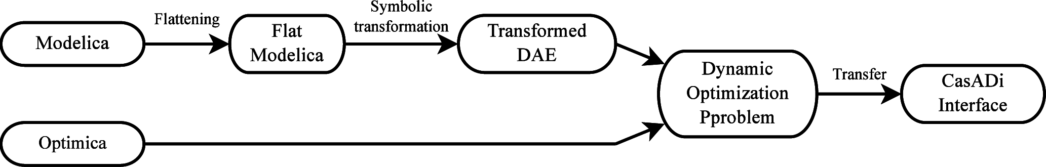
The presented collocation framework is implemented in Python and distributed with JModelica.org [42] under the GNU General Public License. All user interaction takes place in Python, and is centered around the Python interface to CasADi Interface, which serves as a three-way interface between the user, the DOP, and the collocation framework. An overview is illustrated in Figure 3, which begins where the compilation toolchain ends, see Figure 2. After the JModelica.org compiler has transferred the DOP to CasADi Interface, the user can modify it using Python and CasADi, for incorporating constructs that are more conveniently scripted rather than encoded in Modelica and Optimica.
The user can then call upon the collocation framework to solve the DOP, which will transcribe it into an NLP and then solve it using either IPOPT or WORHP, as decided by the user. The user provides options to the collocation framework using a dictionary-like class, specifying things such as discretization scheme, which NLP and linear solver to use, and additional features such as those presented in Section 5. The NLP and linear solver options are also provided directly to the collocation framework. The communication with these solvers is handled by the collocation framework through CasADi’s NLP solver interface, so the user never has to interact with these solvers directly.
The result is stored in a textual format compliant with Dymola [43], one of the most prominent Modelica tools, which is loaded into Python, allowing for convenient extraction of the trajectories. The complete procedure is demonstrated in Section 7.1. Because the hardest part of non-convex optimization is usually to find a suitable initial guess, it is important that initial guesses can be conveniently provided from different sources. To this end, the same result format is used to provide initial guesses, making it convenient to provide initial guesses in the form of optimization or simulation results generated by JModelica.org or Dymola. There have been efforts within the Modelica community to standardize the result format [44]. The usefulness of the implemented framework would be increased if these were to come to fruition.
7. Examples
In this section, we present two examples of how the framework can be used. The first example is a simple optimal control problem based on the Van der Pol oscillator, for which we present the full code used to solve the problem to demonstrate how the framework is used. The second example is optimal control of a large-scale model of a distillation column, which demonstrates the capabilities and performance of the framework. The presented results have been generated using revision [6606] of JModelica.org and IPOPT 3.11.8 with the linear solver MA27. The code used for the second example is lengthy and thus not reproduced in this paper, but it is distributed together with JModelica.org and can be found in pyjmi.examples.distillation4_opt.
Besides the examples discussed in this section, the framework has also been used by both academia and industry to for example estimate kinetic parameters in atomic layer deposition reactors [45], identify models for heating and ventilation in buildings [46] and applying them for MPC [47], optimal control of combined cycle power plants [1,48], and optimal vehicle maneuvers [49].
7.1. Van der Pol Oscillator
The Van der Pol oscillator is a second-order, nonlinear, explicit, ordinary differential equation with a single input, described by
The problem we will solve is to drive the state from (0, 1) towards the origin using a quadratic Lagrange cost on the state and input on a fixed time horizon going from t0 = 0 to tf = 10
This can be encoded in Modelica and Optimica as follows, where we first define the model VDP describing Equation (8). The model is then used to formulate Equation (9) by inheriting it and adding the time horizon, Lagrange cost and input bound on top of it.

This code can then be used to solve the problem using the Python and JModelica.org code below. We first import the compilation methods from JModelica.org, and then compile and simulate the model to generate an initial guess. By not specifying the input values, it defaults to zero, which is sufficient for this simple problem. Next we compile the dynamic optimization problem and solve it for r ∈ {0.1, 1, 10} after setting some solver options. Finally, we simulate the model again, but this time with the different optimal inputs to verify the discretization as discussed in Section 5.3. The obtained trajectories are shown in Figure 4. The plots have been generated using matplotlib [50].
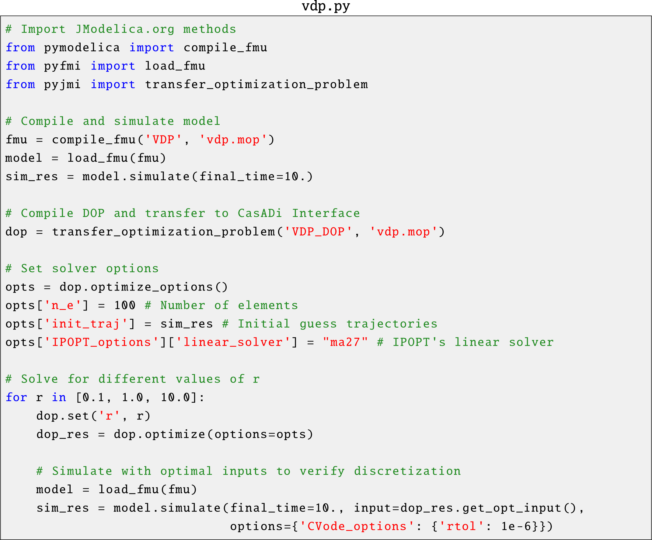
This example demonstrates the flexibility and modularity of the framework. The modeling process is cleanly separated from the solution procedure and the same model is conveniently used to simulate the system to generate initial guess trajectories, solve the optimal control problem, and finally verify the fixed-step collocation discretization by simulating the optimal input. It also shows the interactivity offered by Python scripting, which allows us to easily solve and modify the problem formulation repeatedly in an interactive manner. The small step to setting up an MPC loop is readily envisioned.
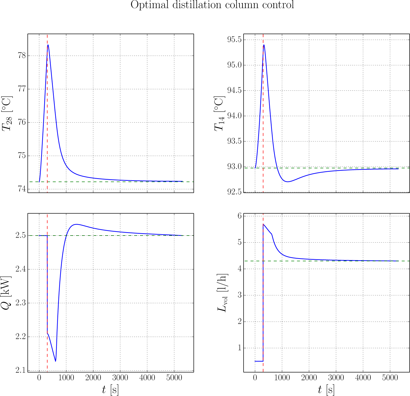
7.2. Distillation Column
The second example is optimal control of a binary distillation column, which separates methanol from n-propanol and has 40 trays. The model was developed in [51] and the Modelica implementation was based on the implementation in [52]. The model is a nonlinear, implicit, DAE system of index one with 125 differential variables and 1000 algebraic variables. The state variables are the temperatures, molar vapor fluxes, and liquid methanol concentrations of each tray, the reboiler, and the condenser.
The control objective is to have a high purity of the distillate and product streams, which is achieved by following a specified constant temperature in two intermediary trays, number 14 and 28, despite disturbances. The system has two inputs: Reboiler heat input Q [°C] and reflux flow rate Lvol [l/h]. There are positivity bounds on the flux out of the condenser and reboiler, which are algebraic variables. These bounds put implicit upper limits on the two system inputs.
The considered scenario is a short reflux breakdown during steady state, where the reflux flow rate is reduced by nearly 90% for 5 minutes, causing the system to drift from the desired steady state. The objective is to steer back to the desired steady state after the breakdown, using quadratic costs on the deviation of the two tray temperatures and input signals from the high-purity steady state.
The problem is discretized using 50 elements with 3 collocation points per element over a horizon of length 5000 seconds, resulting in an NLP with 195,000 variables. The initial guess is constructed by simulating the system with constant input values equal to the reference values. The obtained solution is shown in Figure 5. The entire optimization process, including compilation of the Modelica and Optimica code and construction of AD graphs, takes 87 seconds. 50 of these seconds are spent solving the problem in IPOPT, which solves the problem in 21 iterations. Out of these 50 seconds, 3 seconds are spent evaluating NLP functions and their derivatives by CasADi, and most of the remaining time is spent solving the KKT system in each iteration by MA27. These timings are obtained using pure SX graphs, which uses 1.8 gibibytes of memory. If a mixture of SX and MX graphs are instead used—as discussed in Section 6—the duration of the entire optimization process is increased from 87 seconds to 200 seconds. Most of the additional time is needed in the evaluation of the NLP functions and derivatives. On the other hand, the memory use is decreased from 1.8 gibibytes to 1.1 gibibytes.
8. Conclusions
We have presented the dynamic optimization framework in the open-source platform JModelica.org. The framework solves problems formulated using the modeling language Modelica and its extension Optimica. The framework implements a method based on direct local collocation, of which the details have been discussed based on the Radau scheme. The implementation uses CasADi to construct the nonlinear program in order to efficiently obtain derivative information using algorithmic differentiation, and also to get convenient access to state-of-the-art nonlinear programming numerical solvers. The use of the framework has been demonstrated on a simple optimal control problem. The performance of the framework has also been evaluated on an industrially relevant model of a distillation column.
Potential extensions to the framework are to complement the direct collocation method with a multiple shooting method, and also to extend the mathematical class of supported problems. Developments planned for the immediate future are to extend the symbolical processing of the dynamic optimization problem to decrease the number of equations solved numerically, as discussed in [53].
Acknowledgments
This work was supported by the Swedish Research Council through the LCCC Linnaeus Center. Fredrik Magnusson is a member of the eLLIIT Excellence Center at Lund University. Toivo Henningsson at Modelon AB, Lund, Sweden is acknowledged for his participation in fruitful discussions and work on CasADi Interface.
Author Contributions
Fredrik Magnusson wrote the manuscript and implemented the collocation framework and its integration with the surrounding JModelica.org toolchain. Both authors contributed to the framework design and the conception of the paper.
Conflicts of Interest
The authors declare no conflict of interest.
References
- Sällberg, E.; Lind, A.; Velut, S.; Åkesson, J.; Gallardo Yances, S.; Link, K. Start-Up Optimization of a Combined Cycle Power Plant, Proceedings of the 9th International Modelica Conference, Munich, Germany, 3–5 September 2012.
- Prata, A.; Oldenburg, J.; Kroll, A.; Marquardt, W. Integrated scheduling and dynamic optimization of grade transitions for a continuous polymerization reactor. Comput. Chem. Eng. 2008, 32, 463–476. [Google Scholar]
- Ilzhoefer, A.; Houska, B.; Diehl, M. Nonlinear MPC of kites under varying wind conditions for a new class of large-scale wind power generators. Int. J. Robust Nonlinear Control 2007, 17, 1590–1599. [Google Scholar]
- Zavala, V.M. Inference of building occupancy signals using moving horizon estimation and Fourier regularization. J. Proc. Cont. 2014, 24, 714–722. [Google Scholar]
- Allgöwer, F.; Badgwell, T.A.; Qin, J.S.; Rawlings, J.B.; Wright, S.J. Nonlinear Predictive Control and Moving Horizon Estimation—An Introductory Overview. In Advances in Control: Highlights of ECC ’99; Frank, P.M., Ed.; Springer: Berlin, Germany, 1999; pp. 391–449. [Google Scholar]
- Åkesson, J.; Årzén, K.E.; Gäfvert, M.; Bergdahl, T.; Tummescheit, H. Modeling and optimization with Optimica and JModelica.org—Languages and tools for solving large-scale dynamic optimization problems. Comput. Chem. Eng. 2010, 34, 1737–1749. [Google Scholar]
- JModelica.org User Guide. Available online: http://www.jmodelica.org/page/236 accessed on 16 June 2015.
- Fritzson, P. Principles of Object-Oriented Modeling and Simulation with Modelica 2.1; Wiley-IEEE Press: Piscataway, NJ, USA, 2004. [Google Scholar]
- Åkesson,, J. Optimica—An Extension of Modelica Supporting Dynamic Optimization, Proceedings of the 6th International Modelica Conference, Bielefeld, Germany, 3–4 March 2008.
- Wächter, A.; Biegler, L.T. On the implementation of a primal-dual interior point filter line search algorithm for large-scale nonlinear programming. Math. Program. 2006, 106, 25–57. [Google Scholar]
- Büskens, C.; Wassel, D. The ESA NLP Solver WORHP. In Modeling and Optimization in Space Engineering; Fasano, G., Pintér, J.D., Eds.; Springer: New York, NY, USA, 2013; Volume 73, pp. 85–110. [Google Scholar]
- Liberzon, D. Calculus of Variations and Optimal Control Theory: A Concise Introduction; Princeton University Press: Princeton, NJ, USA, 2012. [Google Scholar]
- Betts, J.T. Practical Methods for Optimal Control and Estimation Using Nonlinear Programming, 2nd ed; Society for Industrial and Applied Mathematics: Philadelphia, PA, USA, 2010. [Google Scholar]
- Bertsekas, D.P. Dynamic Programming and Optimal Control, 3rd ed; Athena Scientific: Belmont, MA, USA, 2005; Volume 1. [Google Scholar]
- Betts, J.T. Survey of numerical methods for trajectory optimization. J. Guid. Contr. Dynam. 1998, 21, 193–207. [Google Scholar]
- Rao, A.V. A Survey of Numerical Methods for Optimal Control, Proceedings of the 2009 AAS/AIAA Astrodynamics Specialists Conference, Pittsburgh, PA, USA, 9–13 August 2009.
- Fourer, R.; Gay, D.M.; Kernighan, B.W. AMPL: A Modeling Language for Mathematical Programming; Duxbury Press Brooks Cole Publishing: Pacific Grove, CA, USA, 2003. [Google Scholar]
- Brooke, A.; Kendrick, D.A.; Meeraus, A.; Rosenthal, R.E. GAMS: A User’s Guide; Scientific Press: Redwood City, CA, USA, 1988. [Google Scholar]
- Hart, W.E.; Laird, C.; Watson, J.P.; Woodruff, D.L. Pyomo – Optimization Modeling in Python; Springer: Berlin, Germany, 2012. [Google Scholar]
- Houska, B.; Ferreau, H.J.; Diehl, M. ACADO toolkit—An open-source framework for automatic control and dynamic optimization. Optimal Control Appl. Methods 2011, 32, 298–312. [Google Scholar]
- Tomlab Optimization. PROPT. Available online: http://tomdyn.com accessed on 16 June 2015.
- Holmström, K. The TOMLAB Optimization Environment in Matlab. Adv. Model. Optim. 1999, 1, 47–69. [Google Scholar]
- Hedengren, J.D. APMonitor. Available online: http://apmonitor.com accessed on 16 June 2015.
- Process Systems Enterprise. gPROMS. Available online: http://www.psenterprise.com/gproms accessed on 16 June 2015.
- Bachmann, B.; Ochel, L.; Ruge, V.; Gebremedhin, M.; Fritzson, P.; Nezhadali, V.; Eriksson, L.; Sivertsson, M. Parallel Multiple-Shooting and Collocation Optimization with OpenModelica, Proceedings of the 9th International Modelica Conference, Munich, Germany, 3–5 September 2012.
- Pytlak, R.; Tarnawski, T.; Fajdek, B.; Stachura, M. Interactive dynamic optimization server—connecting one modelling language with many solvers. Optim. Methods Softw. 2014, 29, 1118–1138. [Google Scholar]
- ITEA. Model Driven Physical Systems Operation. Available online: https://itea3.org/project/modrio.html accessed on 16 June 2015.
- Andersson, J. A General-Purpose Software Framework for Dynamic Optimization. Ph.D. Thesis, KU Leuven, Leuven, Belgium, October 2013. [Google Scholar]
- Andersson, J.; Åkesson, J.; Casella, F.; Diehl, M. Integration of CasADi and JModelica.org, Proceedings of the 8th International Modelica Conference, Dresden, Germany, 20–22 March 2011.
- Magnusson, F.; Åkesson, J. Collocation Methods for Optimization in a Modelica Environment, Proceedings of the 9th International Modelica Conference, Munich, Germany, 3–5 September 2012.
- Åkesson, J.; Ekman, T.; Hedin, G. Implementation of a Modelica compiler using JastAdd attribute grammars. Sci. Comput. Program. 2010, 75, 21–38. [Google Scholar]
- Ekman, T.; Hedin, G. The JastAdd system—modular extensible compiler construction. Sci. Comput. Program. 2007, 69, 14–26. [Google Scholar]
- Mattsson, S.E.; Söderlind, G. Index Reduction in Differential-Algebraic Equations Using Dummy Derivatives. SIAM J. Sci. Comput. 1993, 14, 677–692. [Google Scholar]
- Lennernäs, B. A CasADi Based Toolchain for JModelica.org. M.Sc. Thesis, Lund University, Lund, Sweden, 2013. [Google Scholar]
- HSL. A collection of Fortran codes for large scale scientific computation. Available online: http://www.hsl.rl.ac.uk accessed on 16 June 2015.
- Biegler, L.T. Nonlinear Programming: Concepts, Algorithms, and Applications to Chemical Processes; Mathematical Optimization Society and the Society for Industrial and Applied Mathematics: Philadelphia, PA, USA, 2010. [Google Scholar]
- Hairer, E.; Wanner, G. Solving Ordinary Differential Equations II: Stiff and Differential-Algebraic Problems, 2nd ed; Springer-Verlag: Berlin, Germany, 1996. [Google Scholar]
- Rodriguez, J.S. Large-scale dynamic optimization using code generation and parallel computing. M.Sc. Thesis, KTH Royal Institute of Technology, Stockholm, Sweden, 2014. [Google Scholar]
- Magnusson, F. Collocation Methods in JModelica.org. M.Sc. Thesis, Lund University, Lund, Sweden, February 2012. [Google Scholar]
- Betts, J.T.; Huffman, W.P. Mesh refinement in direct transcription methods for optimal control. Optim. Control Appl. Methods 1998, 19, 1–21. [Google Scholar]
- Vasantharajan, S.; Biegler, L.T. Simultaneous strategies for optimization of differential-algebraic systems with enforcement of error criteria. Comput. Chem. Eng. 1990, 14, 1083–1100. [Google Scholar]
- JModelica.org source code. Available online: https://svn.jmodelica.org and in particular https://svn.jmodelica.org/trunk/Python/src/pyjmi/optimization/casadi_collocation.py?p=6606 accessed on 16 June 2015.
- Dassault Systèmes. Dymola. Available online: http://www.dymola.com accessed on 16 June 2015.
- Pfeiffer, A.; Bausch-Gall, I.; Otter, M. Proposal for a Standard Time Series File Format in HDF5, Proceedings of the 9th International Modelica Conference, Munich, Germany, 3–5 September 2012.
- Holmqvist, A.; Törndahl, T.; Magnusson, F.; Zimmermann, U.; Stenström, S. Dynamic parameter estimation of atomic layer deposition kinetics applied to in situ quartz crystal microbalance diagnostics. Chem. Eng. Sci. 2014, 111, 15–33. [Google Scholar]
- De Coninck, R.; Magnusson, F.; Åkesson, J.; Helsen, L. Grey-Box Building Models for Model Order Reduction and Control, Proceedings of the 10th International Modelica Conference, Lund, Sweden, 10–12 March 2014.
- Vande Cavey, M.; De Coninck, R.; Helsen, L. Setting Up a Framework for Model Predictive Control with Moving Horizon State Estimation Using JModelica, Proceedings of the 10th International Modelica Conference, Lund, Sweden, 10–12 March 2014.
- Larsson, P.O.; Casella, F.; Magnusson, F.; Andersson, J.; Diehl, M.; Akesson, J. A Framework for Nonlinear Model-Predictive Control Using Object-Oriented Modeling with a Case Study in Power Plant Start-Up, Proceedings of the 2013 IEEE Multi-Conference on Systems and Control, Hyderabad, India, 27–30 August 2013.
- Berntorp, K.; Olofsson, B.; Lundahl, K.; Nielsen, L. Models and methodology for optimal trajectory generation in safety-critical road-vehicle manoeuvres. Veh. Syst. Dyn. 2014, 52, 1304–1332. [Google Scholar]
- Hunter, J.D. Matplotlib: A 2D Graphics Environment. Comput. Sci. Eng. 2007, 9, 90–95. [Google Scholar]
- Diehl, M. Real-Time Optimization for Large Scale Nonlinear Processes. Ph.D. Thesis, Heidelberg University, Heidelberg, Germany, July 2001. [Google Scholar]
- Hedengren, J.D. A Nonlinear Model Library for Dynamics and Control, 2008. Available online: http://www.hedengren.net/research/Publications/Cache_2008/NonlinearModelLibrary.pdf accessed on 16 June 2015.
- Magnusson, F.; Berntorp, K.; Olofsson, B.; Åkesson, J. Symbolic Transformations of Dynamic Optimization Problems, Proceedings of the 10th International Modelica Conference, Lund, Sweden, 10–12 March 2014.
Figure 1.
Numerical methods for dynamic optimization. Indirect methods establish optimality conditions first and then discretize the differential equations, whereas direct methods first discretize and then optimize. Both categories of methods use essentially the same discretization techniques, of which the most common ones are single shooting, multiple shooting, and collocation.
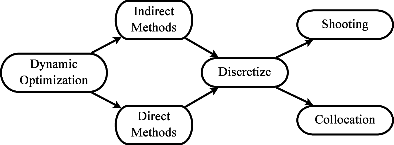
Figure 2.
The compilation process in JModelica.org for DOPs. The process starts with the user-provided Modelica and Optimica code and ends with a symbolic representation of the DOP in CasADi Interface, which serves as an interface between dynamic optimization algorithms and the Modelica and Optimica code.

Figure 3.
The framework surrounding the implemented collocation framework in JModelica.org. The framework starts with a representation of the DOP in CasADi Interface generated by the compiler. The DOP is then discretized by the collocation framework into an NLP, which is solved by either IPOPT or WORHP.
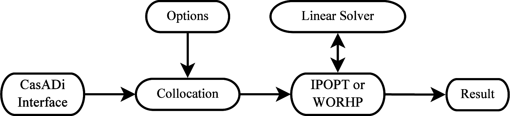
Figure 4.
Optimal control of the Van der Pol oscillator. The initial state is (0, 1) and the objective is a quadratic penalty on the state and input.
Figure 4.
Optimal control of the Van der Pol oscillator. The initial state is (0, 1) and the objective is a quadratic penalty on the state and input.
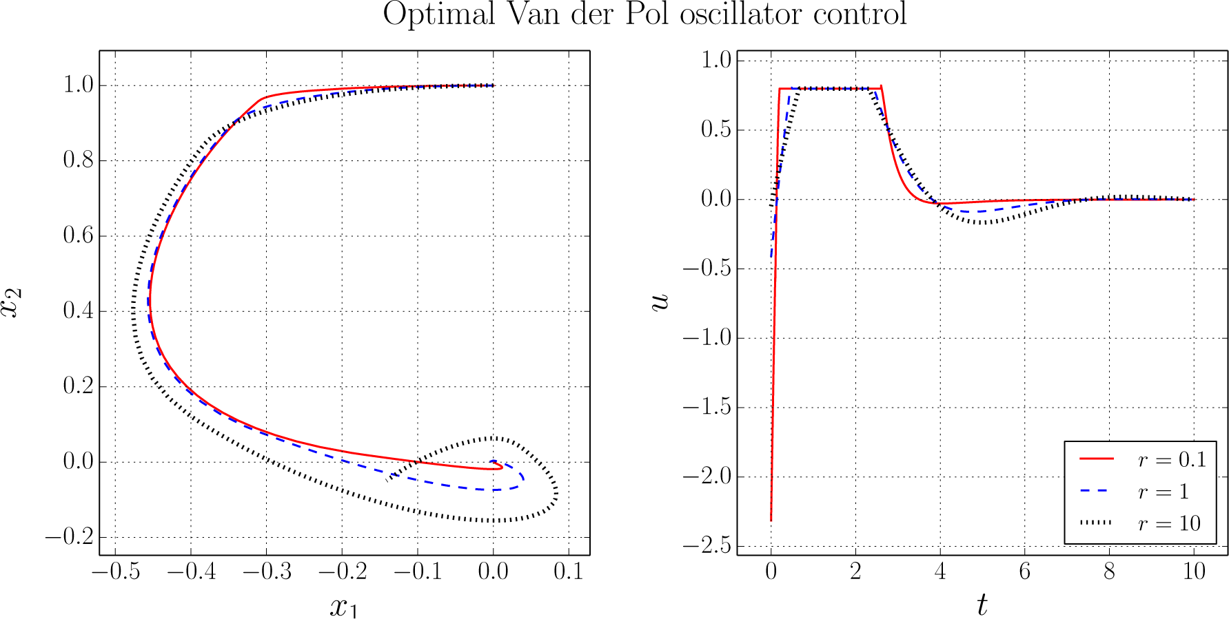
Figure 5.
Control of a distillation column after a reflux breakdown. The vertical dashed lines mark the end of the breakdown, after which the optimal control starts. The horizontal dashed lines mark the reference values, which is the steady state before breakdown.
Figure 5.
Control of a distillation column after a reflux breakdown. The vertical dashed lines mark the end of the breakdown, after which the optimal control starts. The horizontal dashed lines mark the reference values, which is the steady state before breakdown.

© 2015 by the authors; licensee MDPI, Basel, Switzerland This article is an open access article distributed under the terms and conditions of the Creative Commons Attribution license (http://creativecommons.org/licenses/by/4.0/).
Share and Cite
MDPI and ACS Style
Magnusson, F.; Åkesson, J. Dynamic Optimization in JModelica.org. Processes 2015, 3, 471-496. https://doi.org/10.3390/pr3020471
AMA Style
Magnusson F, Åkesson J. Dynamic Optimization in JModelica.org. Processes. 2015; 3(2):471-496. https://doi.org/10.3390/pr3020471
Chicago/Turabian StyleMagnusson, Fredrik, and Johan Åkesson. 2015. "Dynamic Optimization in JModelica.org" Processes 3, no. 2: 471-496. https://doi.org/10.3390/pr3020471