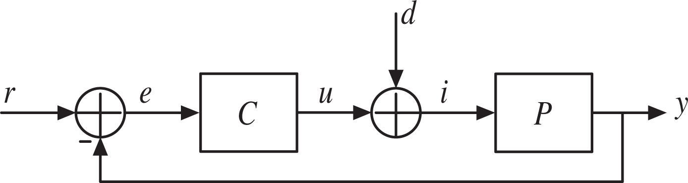
Review

Deterministic Performance Assessment and Retuning of Industrial Controllers Based on Routine Operating Data: Applications

by
Massimiliano Veronesi
1 and
Antonio Visioli
2,*
1
Yokogawa Italia srl, Via Assunta 61, 20834 Nova Milanese (MB), Italy
2
Dipartimento di Ingegneria Meccanica e Industriale, University of Brescia, Via Branze 38, 25123 Brescia, Italy
*
Author to whom correspondence should be addressed.
Processes 2015, 3(1), 113-137; https://doi.org/10.3390/pr3010113
Submission received: 30 December 2014 / Revised: 2 February 2015 / Accepted: 10 February 2015 / Published: 17 February 2015
(This article belongs to the Special Issue Process Control: Current Trends and Future Challenges)

Abstract

:
Performance assessment and retuning techniques for proportional-integral-derivative (PID) controllers are reviewed in this paper. In particular, we focus on techniques that consider deterministic performance and that use routine operating data (that is, set-point and load disturbance step signals). Simulation and experimental results show that the use of integrals of predefined signals can be effectively employed for the estimation of the process parameters and, therefore, for the comparison of the current controller with a selected benchmark.

1. Introduction

Model predictive control has attracted a significant research effort, and it is widely used in industry, because it can optimize the performance of a plant by explicitly taking into account the physical constraints that are present. However, advanced control strategies are often organized hierarchically, with multivariable controllers that provide the set-points to low-level controllers, which are typically of the proportional-integral-derivative (PID) type. Thus, it has to be recognized that the overall process performance relies in any case on the performance of the PID controllers. For this reason, it is important to have tools that are able to automatically assess the performance of a PID controller and, in case it is not satisfactory, to retune the controller in order to optimize the performance. In fact, despite the presence of many effective automatic tuning methodologies based on identification methods suitable for being applied in industry (see, for example, [14]), in many practical cases, PID controllers are poorly tuned, because of the lack of time and skill of the operator. Obviously, especially in large plants where there are hundreds of control loops, it is also important that routine operating data are used, so that no special (possibly time and energy consuming) experiments are needed.
Many performance assessment techniques have been presented in the literature and successfully applied in industry [5]. In general, it is required to compare the current performance with that achieved by a selected benchmark. In this context, even though the proposed techniques can be actually viewed under the same framework (see [6] and the references therein), they are often conveniently divided into two categories [7]: stochastic performance monitoring and deterministic performance monitoring. In the former case, it is important to assess the capability of the control system to deal with stochastic disturbances, and therefore, the control system benchmark is based on the minimum variance concept [810]. In the latter case, more traditional design specifications, such as set-point and load rejection disturbance step response parameters, are considered [11]. In order to provide an effective benchmark, the achievable optimal performance in terms of integrated absolute error for the set-point response has been investigated in [12]. In [13], it is proposed to compare the obtained set-point step response with that achievable by using a PI controller tuned with the internal model control technique. By applying another approach (namely, by avoiding the use of a benchmark system), the so-called Idle Index has been devised in [14] in order to detect sluggish controllers. This idea has been further discussed in [15] and developed in [16], where also guidelines on how to retune the PI controller are given. A comprehensive review of these techniques can be found in [2].
However, it has to be recognized that the selected benchmark system should take into account not only the achievable performance in terms of the minimization of a given index, but also the robustness of the system. Indeed, this is often of main concern by also considering that the control effort is strictly related to it.
In this paper, we review methodologies that have been recently proposed to assess the performance of a PID controller and, based on an estimated model of the system, also retune the controller to achieve the selected benchmark performance. A relevant feature of the presented approach (which will be structured in different contexts) is that it is based on the integral of signals, and it is therefore inherently robust to measurement noise. Simulation and/or experimental results are shown in the different cases in order to illustrate the effectiveness of the techniques.

2. Self-Regulating Processes

2.1. Control Scheme

The unity-feedback control system shown in Figure 1 is considered. The process P is controlled by a PID controller whose transfer function can be either in series (“interacting”) form:
C ( s ) = K p ( T i s + 1 T i s ) ( T d s + 1 ) .
or in ideal (“non-interacting”) form:
C ( s ) = K p ( 1 + 1 T i s + T d s ) .
The use of a (first- or second-order) noise filter [17] is neglected for the sake of simplicity and without loss of generality, by taking into account that it can be designed so that it does not influence the PID controller dynamics significantly.
In order to evaluate the performance of the controller when either a set-point r or a load disturbance d step signal is applied to the control system, an estimation of the process dynamics is performed (then, the current performance is compared with a selected benchmark one). In this context, it is worth recalling the so-called “half rule” [18], as it provides a theoretical background for the proposed methods. The rule states that the largest neglected (denominator) time constant is distributed evenly to the effective dead time and the smallest retained time constant. Thus, for self-regulating processes, the following (possibly high-order) process transfer function can be considered:
P ( s ) = μ Π i ( τ i 0 s + 1 ) e θ 0 s
where the time constants are ordered according to their magnitude (namely, τ10 > τ20 > ⋯). Then, Model (3) can be approximated by a second order plus dead time (SOPDT) transfer function:
P ˜ ( s ) = μ ( τ 1 s + 1 ) ( τ 2 s + 1 ) e θ s
obtained by setting:
τ 1 = τ 10 , τ 2 = τ 20 + τ 30 2 , θ = θ 0 + τ 30 2 + i 4 τ i 0 .
Alternatively, a simpler first order plus dead time (FOPDT) transfer function can be obtained as:
P ˜ ( s ) = μ τ s + 1 e θ s
by setting:
τ = τ 1 + τ 2 2 , θ = θ 0 + τ 2 2 + i 3 τ i .
It is worth noting that, defining as T0 the sum of the time constants and of the dead time of the process, it results:
T 0 : = i τ i 0 + θ 0 = τ 1 + τ 2 + θ = τ + θ .

2.2. Set-Point Following Performance Assessment

Regarding the set-point following task, consider the PID controller (1) and the process model (4). Then, the Simple Internal Model Control (SIMC) tuning rules [18], which are based on the well-known internal model control (IMC) concept, are selected as those that provide the benchmark performance. Based on them, the PID parameters are selected as:
K p = τ 1 2 μ θ , T i = τ 1 , T d = τ 2 .
As a consequence, it is easy to verify that:
T 0 = T i + T d + T i 2 μ K p .
and that, by approximating the delay term as eθs = 1 − θs, the closed-loop transfer function is:
F ( s ) : = C ( s ) P ˜ ( s ) 1 + C ( s ) P ˜ ( s ) 1 θ s + 1 e θ s
for which the resulting step response 2% settling time is:
T s 2 5 θ
and the step response integrated absolute error is:
I A E = 0 | e ( t ) | d t = 2 A s θ .
where e(t) = r(t) − y(t) and As is the amplitude of the set-point step.
It is therefore necessary to evaluate a closed-loop set-point step response and to verify that Equations (10) and (12) (or, alternatively, Equation (13)) are satisfied, in principle, in order to establish that a PID controller is well tuned. Actually, it has to be pointed out that the use of the integrated absolute error is preferable, because, being based on the integral of a signal, it is more robust to the measurement noise. Then, an estimation θm of the apparent dead time of the system can be performed by considering the time interval from the application of the step signal to the set-point and the time instant when the process output attains 2% of the new set-point value As, namely, when the condition y > 0.02As occurs. In this context, in order to cope with the measurement noise, a simple sensible solution is to define a noise band NB [19] (whose amplitude should be equal to the amplitude of the measurement noise) and to rewrite the condition as y > NB. Then, Expression (13) can be rewritten as:
I A E = 0 | e ( t ) | d t = 2 A s θ m .
With respect to Equation (10), it is necessary to determine the process gain µ and the sum of the lags and of the dead time of the process T0 [20]. The process gain µ can be determined by considering the following trivial relations, which involve the final steady-state value of the control variable u:
lim t + u ( t ) = K p T i 0 e ( t ) d t = A s μ
and, therefore, we have:
μ = A s T i K p 0 e ( t ) d t .
The determination of the sum of the lags and of the dead time of the process can be performed by considering the following variable:
v ( t ) = μ u ( t ) y ( t ) .
By applying the Laplace transform to Equation (17) and by expressing u and y in terms of r, we have:
V ( s ) = μ U ( s ) Y ( s ) = C ( s ) ( μ P ( s ) ) 1 + C ( s ) P ( s ) R ( s ) .
At this point, for the sake of clarity, it is convenient to write the controller and process transfer functions, respectively, as:
C ( s ) = K p T i s C ˜ ( s ) , where C ˜ ( s ) : = ( T i s + 1 ) ( T d s + 1 )
and:
P ( s ) = μ e θ 0 s q ( s ) where q ˜ ( s ) : = i ( τ i 0 s + 1 ) .
Then, Expression (18) can be rewritten as:
V ( s ) = μ K p C ˜ ( s ) T i s q ( s ) + μ K p C ˜ ( s ) e θ 0 s ( q ( s ) e θ 0 s ) R ( s ) .
By applying the final value theorem to the integral of v when a step is applied to the set-point signal, we finally obtain:
lim t + 0 t v ( ξ ) d ξ = lim s 0 s A s s μ K p C ˜ ( s ) T i s q ( s ) + μ K p C ˜ ( s ) e θ 0 s q ( s ) e θ 0 s s = A s lim s 0 { 1 e θ 0 s s + q ( s ) 1 s } = A s ( θ 0 + i τ i 0 ) = A s T 0 .
Thus, the sum of the lags and of the dead time of the process can be obtained by determining the integral of v(t) at the steady state when a step signal is applied to the set-point and by dividing it by the amplitude As of the step.
For the purpose of assessing the controller performance based on Equations (10) and (13), it is worth considering the following performance indices, named, respectively, the sigma index SI and the set-point following performance index SFPI (for a PID controller):
S I = T i + T d + T i 2 μ K p T 0
S F P I P I D = 2 A s θ m 0 | e ( t ) | d t
In principle, the performance obtained by the control system is considered to be satisfactory if SFPIPID = 1. From a practical point of view, however, the controller is considered to be well tuned if the index is greater than a given threshold, which can be taken equal to 0.6. Note that this last value has been selected by considering the SIMC tuning rule applied to many different processes [18], but in any case, another value of the threshold can be selected by the user depending on how tight its control specifications are. If the controller results in being badly tuned, then two cases might occur. If the value of SI is less than one, this means that the current tuning is based on an underestimation of the process lags and/or of the dead time. Thus, an improvement of the performance can be achieved by decreasing the value of Kp and/or by increasing the value of Ti and/or Td (see Equation (10)). On the contrary, if the value of SI is greater than one, this means that the current tuning is based on an overestimation of the process lags and/or of the dead time. Thus, an improvement of the performance can be achieved by increasing the value of Kp and/or by decreasing the value of Ti and/or Td.

2.3. Retuning Algorithm

If the performance provided by the controller results in being unsatisfactory, the PID controller needs to be retuned. This can be done by exploiting the following procedure. The closed-loop step response is evaluated, and θm and T0 have to be calculated according to the technique described in Section 2.2 (see Equation (22)). Then, if an overshoot occurs, the proportional gain Kp is decreased, and the integral time constant Ti and the derivative time constant Td are subsequently calculated by means of Expressions (9) and (10). If the resulting value of Ti is less than the value of Td, then Ti has to be decreased, and the values of Kp and Td are updated again according to Equations (9) and (10). The procedure is iterated until a value Td > 0 is obtained. Conversely, if the closed-loop step response is overdamped (namely, there is no overshoot), the procedure starts by increasing the proportional gain Kp, and then, the same steps of the case with overshoot are applied. By taking into account the considerations made in Section 2.2, a sound measure on how much to initially increase or decrease the parameters is given by the sigma index SI.
Formally, starting from given values of Kp, Ti and Td, the algorithm for retuning the PID controller is described as follows [20].
Retuning algorithm
  • Evaluate a closed-loop set-point step response y(t) and the corresponding control variable u(t), and determine µ, θm and T0.
  • Calculate SI according to Equation (23).
  • Set Kpi = Kp (store the initial value of the proportional gain).
  • If maxt y(t) > As (namely, if there is overshoot), then:
    • Set Kp = Kpi · min{SI, 1/SI}.
    • Set Ti = 2µKpθm.
    • Set T d = T 0 T i T i 2 μ K p.
    • If Ti < Td, then:
      • Set Ti = Ti · max{SI, 1/SI}.
      • Set K p = T i 2 μ θ m.
      • Set T d = T 0 T i T i 2 μ K p.
    • If Td < 0, then:
      • If SI > 1, then set SI = 2SI; else set SI = SI/2.
      • Go to 4(a).
  • If maxt y(t) ≤ As (namely, if there is no overshoot), then:
    • Set Kp = Kpi · max{SI, 1/SI}.
    • Set Ti = 2µKpθm.
    • Set T d = T 0 T i T i 2 μ K p.
    • If Ti < Td, then:
      • Set Ti = Ti · max{SI, 1/SI}.
      • Set K p = T i 2 μ θ m.
      • Set T d = T 0 T i T i 2 μ K p.
    • If Td < 0, then:
      • If SI < 1, then set SI = 2SI; else set SI = SI/2.
      • Go to 5(a).
  • End.
A simpler procedure can be performed by considering the FOPDT model (6) and by directly applying the SIMC tuning rules devised for this kind of process, based on the estimated values, θm and τ = T0θm:
K p = T 0 θ m 2 μ θ m , T i = T 0 θ m .

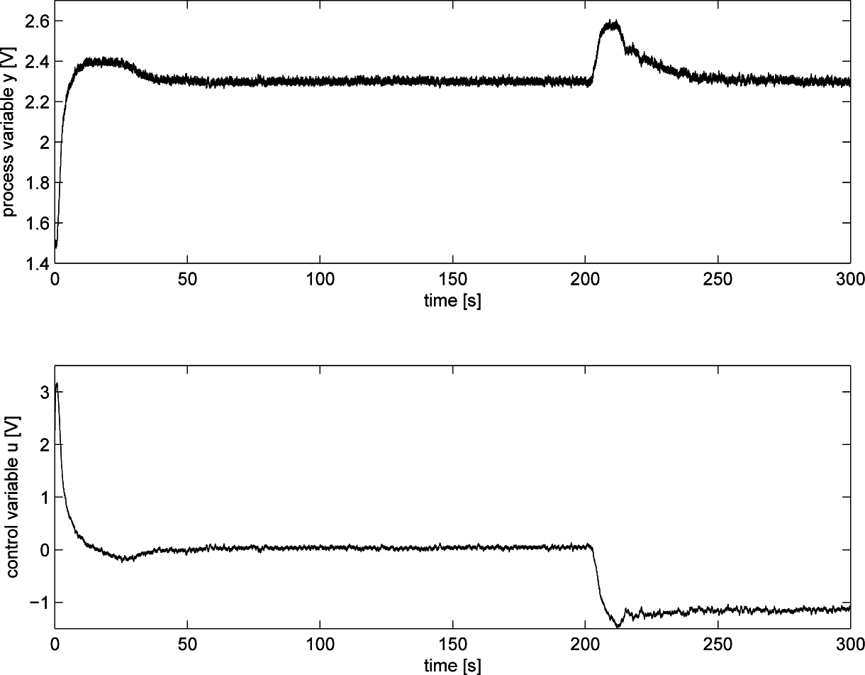
2.4. Experimental Results

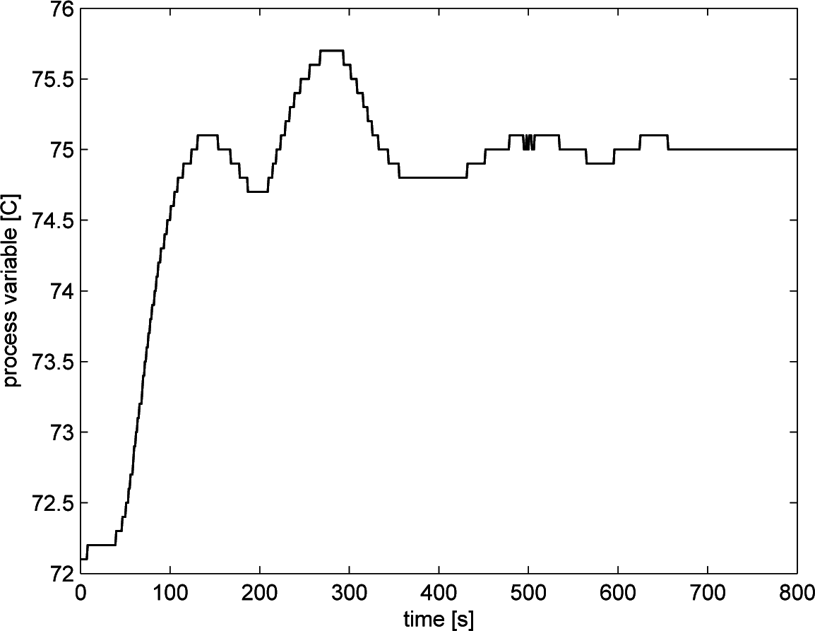
The proposed algorithm has been applied to the temperature control loop shown in Figure 2 as TIC3206. The plant is dedicated to the production of energy from renewable sources, in particular by using palm oil as a fuel. The control task consists of keeping the palm oil pipes at the required (warm) temperature to avoid its solidification, which would cause serious damage to the plant. During routine operations, the system has to keep the steady-state value, but during the start-up phase, the controller must follow a set-point step signal effectively. In the experiments performed on the plant, the controller was initially tuned with a proportional band PB = 70% (note that the proportional band is equal to 100/Kp) and an integral time constant equal to Ti = 70 (s) (Td = 0). After the application of the step signal to the set-point, the process parameters have been determined as θm = 94 (s), µ = 0.285 and T0 = 184.3 (s). The corresponding values of SI and SFPIPID have been determined as 0.84 and 0.545, respectively, indicating the need for a retuning. By applying the retuning algorithm, the new values of the PID controller have been determined as PB = 82.78%, Ti = 64.82 (s) and Td = 24.45 (s), with a corresponding value of SFPIPID = 0.973 (obviously, it is SI = 1). The set-point step responses before and after the retuning procedure are shown in
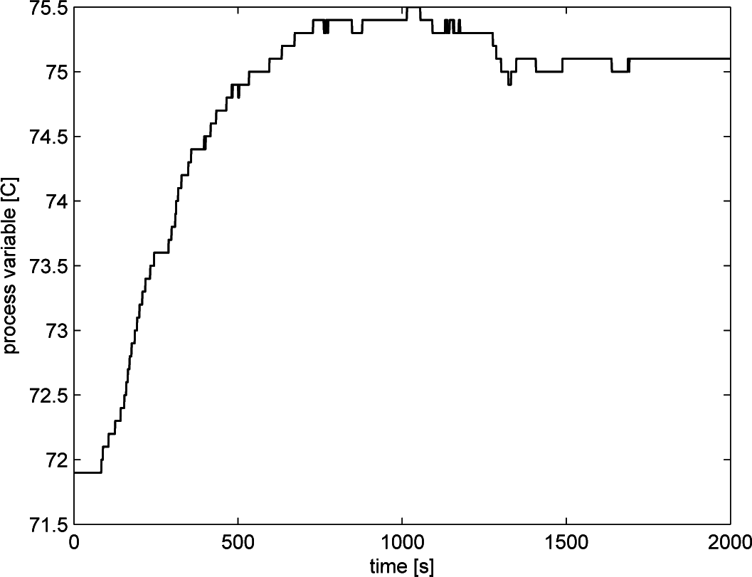
 Figures 3 and 4, respectively, where a clear improvement in the performance appears (note the different time range in the two figures). In particular, the settling time has been considerably reduced, which is obviously appreciated in the start-up phase.
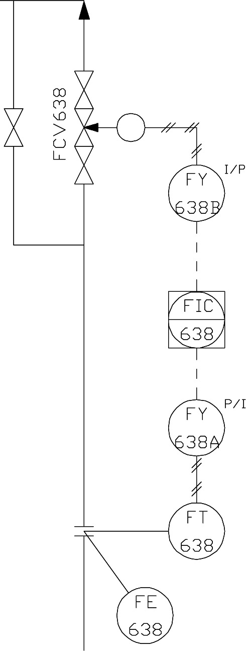
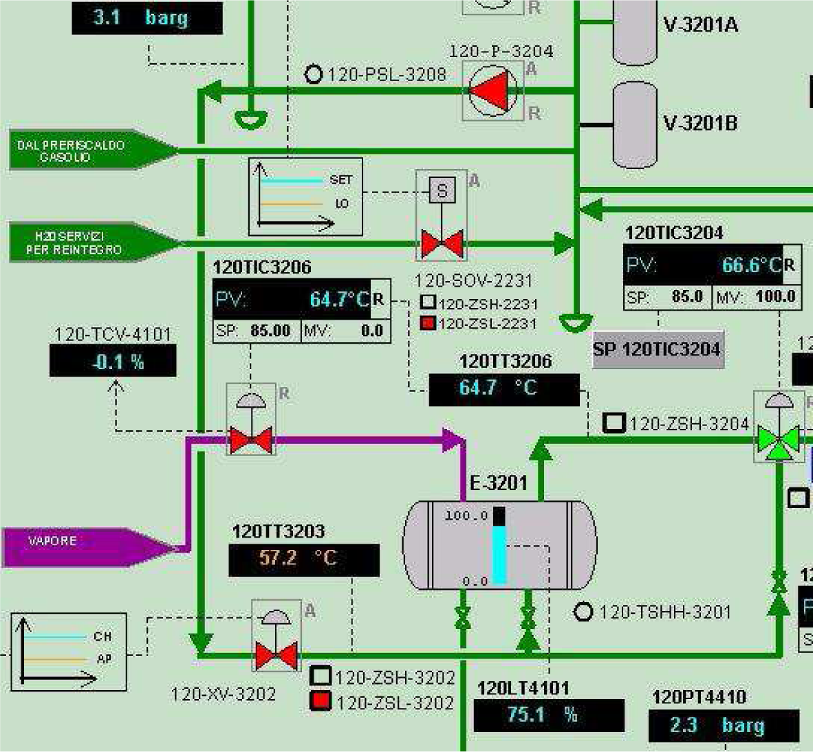
Another experiment has been performed in a chemical plant and, in particular, in a flow control loop denoted as FIC638 in the P&Idiagram shown in Figure 5 [21]. The PI controller controls the flow of hydrochloric acid (HCL), which comes from a tank and is sent to a neutralization column, where it reacts with anhydride-trimethylamine to generate trimethylamine hydrochloride (TMAHCL 56). The FIC638’s performance significantly affects the quality of TMAHCL. Indeed, by providing a fast, but accurate, set-point following, it is possible to avoid the pH correction of the raw product, because the hydrochloride would already be within the designed range.
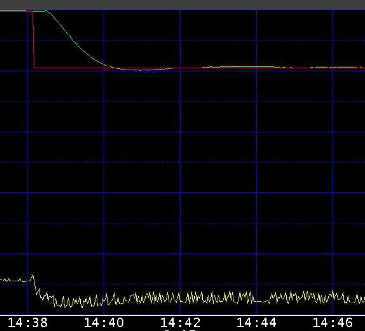
During the commissioning phase, the FIC638 was manually tuned with PB = 500 and Ti = 60 (s), and the resulting response to a set-point step change from 1500 (kg/h) to 1750 (kg/h) was the one shown in Figure 6. The corresponding value of the integrated absolute error (IAE) was 7.585 (kg) (the flow is measured in (kg/h), but the values are stored at each second). When the system attained its steady-state value, the following values of the process parameters were estimated: θm = 19 (s), µ = 3.125 and T0 = 58 (s). The value of the sigma index SI resulted in being 1.86, while the value of the closed-loop index SFPIPID resulted in being equal to 0.35, which means that both indices indicate that the controller had to be retuned. The PI controller has then to be retuned by applying Formula (25), which yielded PB = 304.5 and Ti = 39 (s). These values were applied to the PI controller before changing the set-point value from 1750 (kg/h) back to the value it had previously (1,500 (kg/h)). The step response obtained is shown in Figure 7. It can be seen that, although a small overshoot appeared, the settling time was shorter. The value of the integrated absolute error IAE decreased to 4.01 (kg), and the set-point following performance index increased to 0.66.

2.5. Load Disturbance Rejection Performance Assessment

The same reasoning made for the set-point following performance can be done also for the load disturbance rejection one [22]. Consider the control scheme of Figure 1, where the PID controller has transfer function (2) and the FOPDT process has transfer function (3). A load disturbance step d of amplitude Ad is assumed to enter into the process at a known time instant, which is taken as t = 0 without loss of generality. The disturbance amplitude Ad can be estimated by considering the final value of the integral of the control error:
A s = K p T i 0 e ( t ) d t .
Once the amplitude of the step disturbance has been determined, the process gain µ can be determined, by considering the integral of process input i = u + d (where d = Ad) as:
μ = A d T i K p 0 ( u ( t ) + A d ) d t .
Finally, the value of the sum of the time constants of the process can be determined by considering the variable:
w ( t ) : = μ ( u ( t ) + d ( t ) ) y ( t )
and by calculating T0 as:
T 0 = K p T i A d 0 0 t w ( ξ ) d ξ d t .
Finally, in order to obtain a FOPDT model of the process, the apparent dead time θm of the system can be estimated by considering the time interval from the occurrence of the load disturbance and the time instant when the absolute value of the difference between the process output and its previous steady-state value exceed the noise band threshold.
It is worth stressing that the method works well when an abrupt (namely, step-like) load disturbance occurs. Thus, the performance assessment technique has to be implemented together with a procedure for the detection of abrupt load disturbances, such as, for instance, the one proposed in [23].
Once the process parameters have been estimated, the Chen–Seborg tuning rule proposed in [24] can be used to provide the benchmark performance in terms of integrated absolute error. Indeed, this tuning rule aims at achieving the following closed-loop transfer function (this can be easily ascertained by approximating the delay term as e s θ ( 1 s θ 2 ) / ( 1 + s θ 2 ) ):
Y ( s ) D ( s ) = T i K p ( 1 + s θ / 2 ) s e s θ ( 1 + s τ c ) 3
where τc is a design parameter, which can be selected as τc = θ in order to provide a satisfactory robustness.
Thus, by considering τ = T0θm, the PID controller parameters can be calculated as:
K p = 28 T 0 41 θ m 27 μ θ m , T i = θ m 4 28 T 0 41 θ m 2 T 0 θ m , T d = θ m ( 11 T 0 19 θ m ) 28 T 0 41 θ m .
As the desired closed-loop transfer function (30) has only real poles, the desired integrated absolute error IAE is equal to the integrated error, that is (see Equation (26)):
I A E = A d T i K p .
By replacing Kp and Ti in Equation (32) with the values in Equation (31), it results:
I A E = 27 A d μ θ m 2 4 ( 2 T 0 θ m ) .
Thus, a performance index for the load rejection task (called LRPI, load disturbance rejection performance index) for a PID controller is defined by comparing the obtained integrated absolute error with the desired one, that is:
L R P I P I D = 27 A d μ θ m 2 4 ( 2 T 0 θ ) 0 | e ( t ) | d t .
A similar reasoning can be applied if a PI controller is selected. In this case, the target closed-loop transfer function between the process variable and the load disturbance is:
Y ( s ) D ( s ) = T i K p s e s θ ( 1 + s τ c ) 2
where τc = θ to achieve a satisfactory robustness. Correspondingly, by considering the estimated apparent dead time, the tuning formulas are:
K p = T i T 0 4 μ θ m 2 , T i = θ m ( 3 T 0 4 θ m ) T 0
and the performance index is:
L R P I P I = 4 A d μ θ m 2 T 0 0 | e ( t ) | d t
As for the set-point following performance, even if the ideal LRPI index is equal to one, from a practical point of view, a sensible default value of 0.6 can be imposed, but in any case, the value of the threshold can be selected by the user depending on how tight the required performance in a given application is.
It is worth noting at this point that, despite the tuning of the PID controller taking into account the load disturbance rejection task, the set-point following performance can be in any case recovered by considering that, for PID controllers, the transfer function from the reference signal to the process variable is:
F ( s ) = Y ( s ) R ( s ) = ( T i T d s 2 + T i s + 1 ) ( 1 + θ 2 s ) ( 1 + s θ ) 3 e θ s .
Thus, by adopting a two degrees of freedom PID controller, a set-point filter equal to:
H ( s ) = a T i T d s 2 + b T i s + 1 ( T i T d s 2 + T i s + 1 ) ( 1 + θ 2 s )
can be designed by placing both zeros at −1/θ, so that the overall transfer function between the set-point and the process variable now results:
F ˜ ( s ) = H ( s ) F ( s ) = e s θ 1 + θ s .
This is achieved by setting:
b = 2 θ T i , a = T i b 2 4 T d = 1 θ .
By following a similar reasoning for the PI controller case, the set-point filter has to be designed as:
H ( s ) = θ s + 1 1 + s T i .
Thus, in this context, as the overall transfer function is of the FOPDT type, the set-point following performance can be assessed by using the performance index of Equation (24).
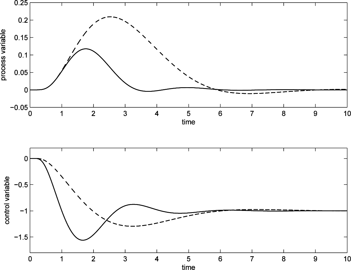
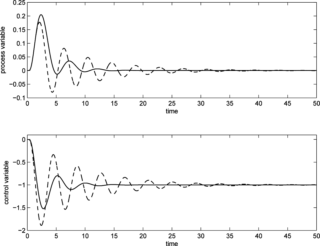
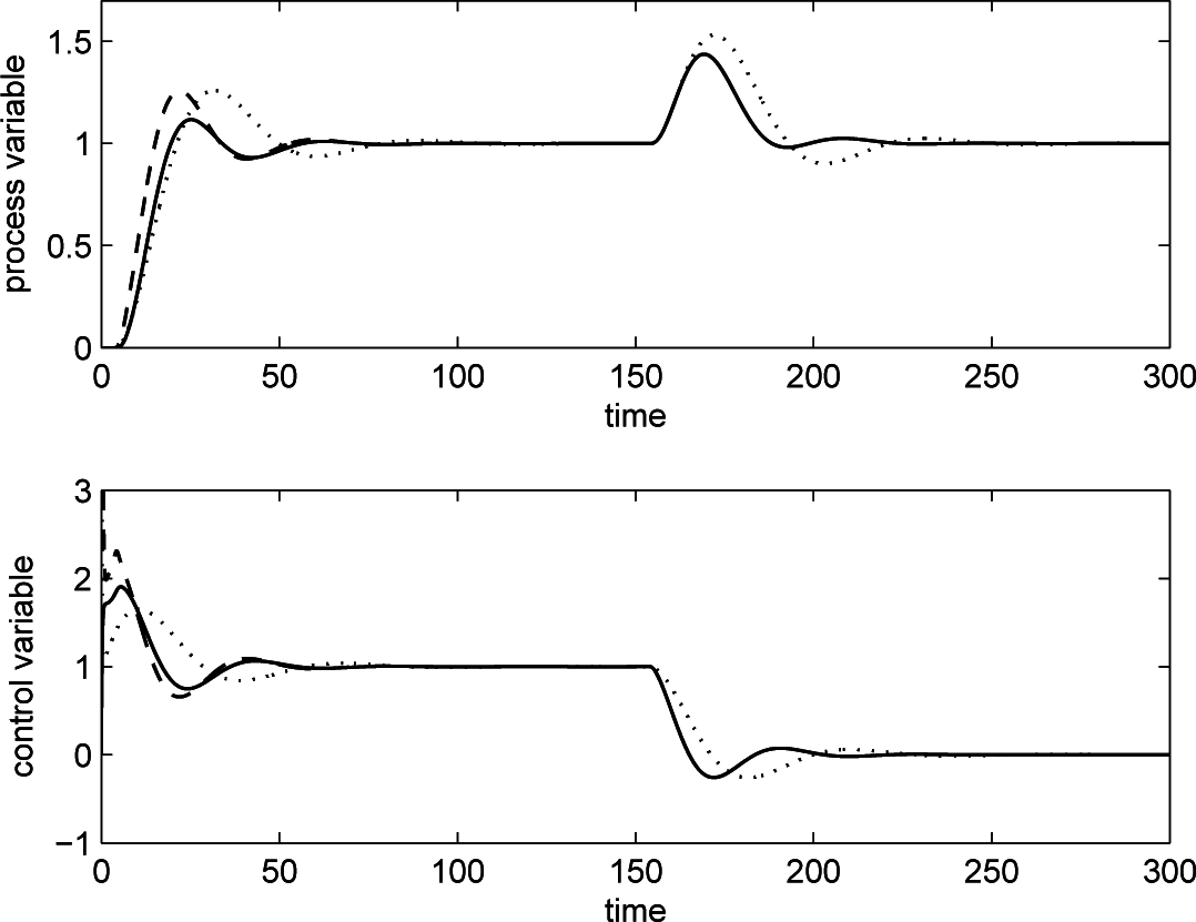
As an illustrative example, consider the process:
P ( s ) = e 4 s ( 10 s + 1 ) ( 5 s + 1 ) ( s + 1 ) .
A PID controller is initially employed with the parameters selected as Kp = 1, Ti = 10 and Td = 1. After the load disturbance occurs on the process, the gain µ is correctly determined by means of Equation (72), while the computation (73) gives exactly T0 = 20; finally, the dead time is estimated to be θm = 6.27. The performance indices related to this initial manual tuning are LRPIPID = 0.582 and SFPIPID = 0.642, which indicates a quite poor behavior of the controller. Hence, the PID parameters are retuned by using Equation (36), resulting in Kp = 1.785, Ti = 14.06, Td = 2.087. Figure 8 shows the performance improvement that results from the retuning; of course, when the set-point filter of Equation (42) is applied, the typical aggressiveness in the load disturbance rejection task does not have to be paid by a high overshoot in the set-point following, like happens if the filter is not used. In fact, in both cases, it is LRPIPID = 0.877, but by filtering the set-point, it is SFPIPID = 0.849.

3. Distributed Lag Processes

3.1. Modeling

Distributed lag processes are frequently encountered in the process industry. For example, transmission lines, heat exchangers, stirred tanks and distillation columns might have a dynamic characteristic, so that they can be modeled as an infinite series of infinitesimally small interacting lags and, therefore, as a distributed lag [25].
A distributed lag process can be described by the following transfer function:
P ( s ) = 2 μ e τ s + e τ s = μ cosh τ s
where µ is the process gain. The hyperbolic cosine can be expanded into an infinite product series, so that it results:
P ( s ) = μ [ 1 + ( 2 / π ) 2 τ s ] [ 1 + ( 2 / 3 π ) 2 τ s ] [ 1 + ( 2 / 5 π ) 2 τ s ]
Note that, for the purpose of simulation, the transfer function (45) can be written as:
P ( s ) = μ i = 0 n 1 [ 1 + ( 2 ( 2 i + 1 ) π ) 2 τ s ]
with n at least equal to 20, because the dynamics of the process does not change significantly for n > 20 [26]. It is worth noting that the sum of all time constants, denoted as T0, is equal to 0.5τ. The sum of all time constants can be estimated easily, by means of an open-loop step response, as the time the process variable takes to attain 63.2% of its steady-state value, and the process gain can be determined by considering the steady-state value of the process output and the amplitude of the step input.
However, in order to avoid stopping the routine process operations, also for this kind of processes, T0 and µ can be estimated with a closed-loop experiment, namely by employing a PID controller with any values of the parameters (provided that the closed-loop system is asymptotically stable).
Considering the control scheme of Figure 1 and the PID controller (1), the same formulas employed in Section 2, both for the evaluation of a set-point and the load disturbance step signal, can be applied also in this case [27].

3.2. Performance Assessment and Retuning for Load Disturbance Rejection

The PI(D) controller tuned according to the rules devised by Shinskey [25,26] can be effectively employed to select the benchmark performance in case a load disturbance has to be rejected. In the case of a PI controller, the parameters can be selected as Kp = 5/µ and Ti = 0.54T0, while, in the case of a PID controller, it is Kp = 100/15/µ, Ti = 0.25T0 and Td = 0.10T0. The benchmark performance, in terms of integrated absolute error, can be determined by applying these tuning rules to many (simulated) distributed lag processes (45) with different values of µ and τ and different process order n. Results for µ = 1 are shown in Figures 9 and 10 for PI and PID controllers, respectively. By interpolating the results, the following values of IAE are obtained (for PI and PID controllers, respectively):
I A E P I = 0.058 τ μ = 0.116 T 0 μ
I A E P I D = 0.02 τ μ = 0.04 T 0 μ
Thus, a performance index for a PI and a PID controller, respectively, can be defined as:
L R P I P I = 0.116 T 0 μ 0 | e ( t ) | d t
L R P I P I D = 0.04 T 0 μ 0 | e ( t ) | d t
By performing many simulations, it has been found that, even if, in principle, it should be LRPIPI = 1 or LRPIPID = 1, the controller can be considered to be well tuned if the index is greater than 0.8.
It is worth noting in any case that the use of the derivative action allows a significant improvement of the performance.

3.3. Simulation Results

As a first example, consider a process with µ = 1, τ = 10 and n = 30 lags. Initially, the PID controller parameters are selected as Kp = 3.3, Ti = 1.9, Td = 0.25. Then, a unit step load disturbance is applied to the process (see the dashed line in Figure 11), and the amplitude of the disturbance, the gain of the process and the sum of the time constants are estimated as Ad = 1, µ = 1.0 and T0 = 4.97. Based on these values, the PID parameters are retuned, as Kp = 6.66, Ti = 1.24, Td = 0.5. The load disturbance step response provided by the new values of the PID controller parameters is shown as a solid line in Figure 11. By retuning the controller, the performance index is improved from LRPIPID = 0.32 to LRPIPID = 1.03, while the integrated absolute error decreases from IAE = 0.62 to IAE = 0.19. It is worth noting that the same result is achieved if a set-point step response is employed for estimating the process parameters.
Consider now the use of a PI controller for the same process. Initially, an aggressive controller is selected with Kp = 7 and Ti = 2. By evaluating a unit step load disturbance, the gain of the process and the sum of the time constants are estimated as Ad = 1, µ = 0.99 and T0 = 4.97. Based on these values, the PI parameters are retuned as Kp = 5.06 and Ti = 2.68. The load disturbance step responses provided by the initial and new values of the PI controller parameters are shown in Figure 12. The performance index is improved from LRPIPID = 0.64 to LRPIPID = 1.01, while the integrated absolute error decreases from IAE = 0.88 to IAE = 0.56.

4. Integral Processes

4.1. Modeling

The approach devised for self-regulating processes can be also exploited for integral (non self-regulating) processes by applying appropriate modifications [28]. The process can be modeled by means of the following transfer function:
P ( s ) = μ s Π i ( τ i 0 s + 1 ) e θ 0 s
where the time constants are ordered according to their magnitude (namely, τ10 > τ20 >⋯). Then, by applying the “half rule”, a second order plus dead time (SOPDT) transfer function:
P ˜ ( s ) = μ s ( τ 1 s + 1 ) e θ 0 s
is obtained by setting:
τ 1 = τ 10 + τ 20 2 , θ = θ 0 + τ 20 2 + i 3 τ i 0 .
It is worth stressing that, also in this case, the sum of the dead time and of the time constants of the process (51) is unaltered in the reduced model, that is,
T 0 : = i τ i 0 + θ 0 = τ 1 + θ .

4.2. Performance Assessment and Retuning

In order to devise a sensible performance assessment strategy, the different control tasks have to be taken into account, as a different kind of controller results. In particular, it has to be taken into account that, as an integrator is present in the process, a PD controller has be used if only the set-point following performance is addressed, while a PID controller has to be used if load disturbances have to be rejected.
In general, consider the PID controller (1) in series form. If only the set-point following task is of concern, the desired benchmark performance can be suitably selected as that obtained by applying the IMC approach [29], which, if applied to the process (52), where the dead time is approximated as eθs ≅ = 1 − θs, yields a PD controller whose parameters are selected according to the following tuning rule:
K p = 1 2 μ λ , T d = τ 1
where λ is the selected closed-loop time constant and can be selected as λ = θ in order to achieve good robustness. With this PD controller and with the same approximation as before for the dead time term, the closed-loop transfer function results as in (11), and the corresponding integrated absolute error when a step signal of amplitude As applied to the set-point results as in (13). Thus, as in (24), the controller performance with respect to the set-point following task can be assessed by considering the following performance index:
S F P I P D = 2 A s θ m 0 | e ( t ) | d t .
If both the set-point following and the load disturbance rejection are of concern in the control task, the integral action has to be employed in order to achieve a null steady-state error in the presence of a constant load disturbance. In this case, the desired performance can be suitably selected as the one obtained by applying the SIMC tuning rule [18]:
K p = 1 2 μ θ , T i = 8 θ , T d = τ 1 .
In this case, the complementary sensitivity transfer function results in being:
F ( s ) = Y ( s ) R ( s ) = C ( s ) P ˜ ( s ) 1 + C ( s ) P ˜ ( s ) ( 1 + 8 θ s ) e θ s 8 θ 2 s 2 + 7 θ s + 1
whereas, after trivial calculations, the transfer function between the load disturbance d and the process output y results in being:
T ( s ) = Y ( s ) D ( s ) = P ˜ ( s ) 1 + C ( s ) P ˜ ( s ) 16 θ 2 μ s ( 8 θ 2 s 2 + 7 θ s + 1 ) ( τ 1 s + 1 ) e θ s .
By considering F(s), the integrated absolute error when a step signal of amplitude As is applied to the set-point can be calculated as [28]:
I A E = 0 | e ( t ) | d t = 3.45 A s θ .
and therefore, the set-point following performance index SFPIPID to assess the controller performance when a step signal is applied to the set-point can be defined as:
S F P I P I D = 3.45 A s θ m 0 | e ( t ) | d t .
Conversely, when a step load disturbance of amplitude Ad occurs, as there are no complex poles in the transfer function T(s) between the load disturbance and the process output, the integrated absolute error can be calculated as:
I A E = I E = T i K p A d = 16 μ θ 2 A d
Hence, the load disturbance response performance index LRPIPID to assess the controller performance when a step load disturbance occurs can be defined as:
L R P I P I D = 16 μ θ m 2 A d 0 | e ( t ) | d t .
Finally, if only the load disturbance rejection performance is of concern, an appropriate tuning rule to be employed for the definition of the benchmark system is the one that aims at minimizing the integrated absolute error, suggested in [25] as:
K p = 0.78 μ ( τ 1 + θ ) , T i = 1.38 ( τ 1 + θ ) , T d = 0.66 ( τ 1 + θ ) .
The corresponding integrated absolute error can be determined with a numerical procedure as:
I A E = A d μ τ 1 2 [ 2.715 + 5.144 ( θ τ 1 ) + 2.266 ( θ τ 1 ) 2 ]
and therefore, the corresponding load disturbance rejection performance index LRPIPID is defined as:
L R P I P I D = A d μ τ 1 2 [ 2.715 + 5.144 ( θ m τ 1 ) + 2.266 ( θ m τ 1 ) 2 ] 0 | e ( t ) | d t .
In all cases, even if it would be desirable to have a value of the performance index equal to one, a suitable threshold can be defined as 0.6.
In order to determine the performance index and to retune the controller (see Equations (55), (57) and (64)), it is necessary to estimate the values of µ, T0 and of the dead time θ, as well as the value of the amplitude of the load step disturbance Ad for the load disturbance case.
The estimated value of the apparent dead time θm of the system can be determined as described in Section 2. Then, if a set-point step response is evaluated, by following again a procedure involving the final value theorem, the determination of the sum of the lags and of the dead time of the process can be obtained as:
T 0 = lim t + 0 t v i ( ξ ) d ξ A s
where:
v i ( t ) : = μ 0 t u ( ξ ) d ξ y ( t ) .
while the process gain µ can be determined as:
μ = A s T i K p 0 0 t e ( ξ ) d ξ d t ,
or, in case the integral action is not employed, as:
μ = A s K p 0 e ( t ) d t .
On the contrary, if a step load disturbance response is evaluated, the amplitude Ad of the step load disturbance can be determined as:
A d = K p T i 0 e ( v ) d v .
Then, the process gain µ can be determined as:
μ = A d T i K p 0 0 t ( u ( v ) + A d ) d v d t .
and the sum of the lags and of the dead time of the process as:
T 0 = K p T i A d 0 0 t w i ( ξ ) d ξ d t .
where:
w i ( t ) : = μ 0 t ( u ( ξ ) + A d ) d ξ y ( t ) .
Note that the time constant τ1 can be calculated as τ1 = T0θm.

4.3. Experimental Results

A laboratory setup, which consists of a small Perspex tower-type tank, has been modified conveniently in order to obtain a level control task with an integral process. The process can be modeled by the following differential equation:
d y ( y ) d t = 1 A u ( t ) .
where y is the level (i.e., the process variable), A is the area of the tank and the control variable u(t) = qi(t) − q0(t) is the difference between the input and output flow rates. An apparent dead time is present in the process because of the neglected dynamics and because of the length of the pipe. A load disturbance is added to the process by applying an additional input flow rate by means of another pump.
The case where both set-point following and load disturbance rejection performance is of concern has been considered. Initially, a PI controller has been implemented by setting Kp = 1 and Ti = 100 (s). The results obtained by applying a set-point step from 1.5 to 2.3 V (namely, As = 0.8) at time t = 0 and a load disturbance at t = 200 are shown in Figure 13. By using the data of the set-point step response, the values θm = 2 (s), T0 = 16.02 (s) and µ = 0.06 have been estimated. The resulting integrated absolute error is IAE = 9.04, and the resulting set-point following performance index is SFPIPID = 0.61. By considering the load disturbance response, the resulting integrated absolute error is IAE = 107.9, and the resulting load disturbance performance index is LRPIPID = 0.05. This latter result indicates that it is worth retuning the controller. By applying the tuning rule (57), the PID parameters have been calculated as Kp = 3.70, Ti = 16 (s) and Td = 0.02 (s). The corresponding results are shown in Figure 14, where the resulting integrated absolute errors are IAE = 4.92 and IAE = 5.93 for the set-point and load disturbance response, respectively. The corresponding performance indices are SFPIPID = 0.84 and LRPIPID = 0.85.

5. Conclusions

Methodologies for the deterministic performance assessment and retuning of PID controllers have been reviewed and presented in a unified way in this paper (see Table 1 for a summary of the developed performance indices). The basic idea, developed for different contexts, is to exploit the final value theorem to estimate the process parameters based on the integral of appropriate signals that results from a set-point or a load disturbance step response. This makes the technique suitable for implementing in industry, as it uses routine operating data, is inherently robust to measurement noise and the result is almost independent of the tuning of the initial controller (on the contrary, standard least squares techniques assume an input signal that significantly excites the dynamics of the system to be estimated). The methodologies analyzed can be implemented with standard Distributed Control Systems software and can also be extended to more complex control techniques, like cascade control [30], dead time compensators [31] and feedforward control [32].

Author Contributions

This paper is a collaborative work between both authors. They both conceived the methodology; M.V. performed the experiments; A.V. wrote the paper.

Conflicts of Interest

The authors declare no conflict of interest.

References

  1. Åström, K.J.; Hägglund, T. Advanced PID Control; ISA Press: Research Triangle Park, NC, USA, 2006. [Google Scholar]
  2. Visioli, A. Practical PID Control; Springer: London, UK, 2006. [Google Scholar]
  3. Visioli, A.; Zhong, Q.C. Control of Integral Processes with Dead Time; Springer: London, UK, 2010. [Google Scholar]
  4. Liu, T.; Gao, F. Industrial Process Identification and Control Design; Springer: London, UK, 2012. [Google Scholar]
  5. Jelali, M. An overview of control performance assessment technology and industrial applications. Control Eng. Pract. 2006, 14, 441–466. [Google Scholar]
  6. Huang, B.; Shah, S. Performance Assessment of Control Loops – Theory and Applications; Springer: London, UK, 1999. [Google Scholar]
  7. Qin, S.J. Control performance monitoring - a review and assessment. Comput. Chem. Eng. 1998, 23, 173–186. [Google Scholar]
  8. Harris, T.J. Assessment of control loop performance. Can. J. Chem. Eng. 1989, 67, 856–861. [Google Scholar]
  9. Ko, B.S.; Edgar, T.F. PID control performance assessment: the single-loop case. AIChE J 2004, 50, 1211–1218. [Google Scholar]
  10. Veronesi, M.; Visioli, A. Global minimum-variance PID control, Proceedings of the 18th IFAC World Congress on Automatic Control, Milan, Italy, 28 August–2 September 2011; pp. 7891–7896.
  11. Eriksson, P.G.; Isaksson, A.J. Some aspects of control loop performance monitoring, Proceedings IEEE Conference on Control Applications, Glasgow, UK, 24–26 August 1994; pp. 1029–1034.
  12. Huang, H.P.; Jeng, J.C.; Chiang, C.H.; Pan, W. A direct method for multi-loop PI/PID controller design. J. Process Control. 2003, 13, 769–786. [Google Scholar]
  13. Swanda, A.P.; Seborg, D.E. Controller performance assessment based on set-point response data, Proceedings of the American Control Conference, San Diego, CA, USA, 4 June 1999; pp. 3863–3867.
  14. Hägglund, T. Automatic detection of sluggish control loops. Control Eng. Pract. 1999, 7, 1505–1511. [Google Scholar]
  15. Kuehl, P.; Horch, A. Detection of sluggish control loops-experiences and improvements. Control Eng. Pract. 2005, 13, 1019–1025. [Google Scholar]
  16. Visioli, A. Method for proportional-integral controller tuning assessment. Ind. Eng. Chem. Res. 2006, 45, 2741–2747. [Google Scholar]
  17. Segovia, V.R.; Hägglund, T.; Åström, K. Measurement noise filtering for common PID tuning rules. Control Eng. Pract. 2014, 32, 43–63. [Google Scholar]
  18. Skogestad, S. Simple analytic rules for model reduction and PID controller tuning. J. Process Control. 2003, 13, 291–309. [Google Scholar]
  19. Åström, K.J.; Hägglund, T.; Hang, C.C.; Ho, W.K. Automatic tuning and adaptation for PID controllers - a survey. Control Eng. Pract. 1993, 1, 699–714. [Google Scholar]
  20. Veronesi, M.; Visioli, A. Performance assessment and retuning of PID controllers. Ind. Eng. Chem. Res. 2009, 48, 2616–2623. [Google Scholar]
  21. Veronesi, M.; Visioli, A. An industrial application of a performance assessment and retuning technique for PI controllers. ISA Trans. 2010, 49, 244–248. [Google Scholar]
  22. Veronesi, M.; Visioli, A. Performance assessment and retuning of PID controllers for load disturbance rejection, Proceedings of the IFAC Conference on Advances in PID Control, Brescia, Italy, 28–30 March 2012; pp. 530–535.
  23. Veronesi, M.; Visioli, A. A technique for abrupt load disturbance detection in process control systems, Proceedings of the 17th IFAC World Congress, Seoul, Korea, 6–11 July 2008; pp. 14900–14905.
  24. Chen, D.; Seborg, D. PI/PID controller design based on direct synthesis and disturbance rejection. Ind. Eng. Chem. Res. 2002, 41, 4807–4822. [Google Scholar]
  25. Shinskey, F.G. Feedback Controllers for the Process Industries; McGraw-Hill: New York, NY, USA, 1994. [Google Scholar]
  26. Shinskey, F.G. PID-deadtime control of distributed processes. Control Eng. Pract. 2001, 9, 1177–1183. [Google Scholar]
  27. Veronesi, M.; Visioli, A. A PID automatic tuning method for distributed-lag processes, Proceedings of the 7th IFAC International Symposium on Advanced Control of Chemical Processes, Istanbul, Turkey, 12–15 July 2009; pp. 762–767.
  28. Veronesi, M.; Visioli, A. Performance assessment and retuning of PID controllers for integral processes. J. Process Control. 2010, 20, 261–269. [Google Scholar]
  29. Rivera, D.E.; Skogestad, S.; Morari, M. Internal model control. 4. PID controller design. Ind. Eng. Chem. Process Des. Dev. 1986, 25, 252–265. [Google Scholar]
  30. Veronesi, M.; Visioli, A. A simultaneous closed-loop automatic tuning method for cascade controllers. IET Control Theory Appl. 2011, 5, 263–270. [Google Scholar]
  31. Normey-Rico, J.E.; Sartori, R.; Veronesi, M.; Visioli, A. An automatic tuning methodology for a unified dead-time compensator. Control Eng. Pract. 2014, 27, 11–22. [Google Scholar]
  32. Veronesi, M.; Visioli, A. Automatic tuning of feedforward controllers for disturbance rejection. Ind. Eng. Chem. Res. 2014, 53, 2764–2770. [Google Scholar]
Figure 1. The control scheme considered.
Processes 03 00113f1
Figure 2. Overview of part of the renewable energy plant used for experimental results.
Processes 03 00113f2
Figure 3. Initial set-point step response in the temperature control loop.
Processes 03 00113f3
Figure 4. Set-point step response after the PID controller retuning in the temperature control loop.
Processes 03 00113f4
Figure 5. The considered flow control loop for the chemical plant.
Processes 03 00113f5
Figure 6. Initial set-point step response in the flow control loop. Top: process variable. Bottom: control variable.
Processes 03 00113f6
Figure 7. Set-point step response after the PID controller retuning in the flow control loop. Top: process variable. Bottom: control variable.
Processes 03 00113f7
Figure 8. Results of the illustrative example for disturbance rejection performance assessment. Dotted line: initial tuning; dashed line: simple PID retuned; solid line: retuned PID plus set-point filter.
Processes 03 00113f8
Figure 9. Values of the integrated absolute error (IAE) for different values of τ and n (process order) with a PI controller tuned according to the benchmark tuning rules.
Processes 03 00113f9
Figure 10. Values of IAE for different values of τ and n (process order) with a PID controller tuned according to the benchmark tuning rules.
Processes 03 00113f10
Figure 11. Load disturbance step response for PID control for a distributed lag process. Dashed line: initial tuning; solid line: after retuning.
Processes 03 00113f11
Figure 12. Load disturbance step response for PI control for a distributed lag process. Dashed line: initial tuning; solid line: after retuning.
Processes 03 00113f12
Figure 13. Experimental results for an integral process: initial tuning.
Processes 03 00113f13
Figure 14. Experimental results for an integral process: after retuning.
Processes 03 00113f14
Table 1. Summary of the performance indices for the different kinds of processes and control tasks.
Process TypeControllerControl TaskPerformance Index
Self-regulatingPI(D)set-point following(24)
Self-regulatingPIDload disturbance rejection(34)
Self-regulatingPIload disturbance rejection(37)
Self-regulatingPI(D) with set-point filterset-point following (and load disturbance rejection)(24)
Distributed-lagPIload disturbance rejection(49)
Distributed-lagPIDload disturbance rejection(50)
Non-self-regulatingPDset-point following(56)
Non-self-regulatingPIDset-point following (and load disturbance rejection)(61)
Non-self-regulatingPIDload disturbance rejection (and set-point following)(63)
Non-self-regulatingPIDload disturbance rejection(66)

