

Generalized Conditional Feedback System with Model Uncertainty

1
State Key Laboratory of Power Systems, Department of Energy and Power Engineering, Tsinghua University, Beijing 100084, China
2
Center for Advanced Control Technologies, Cleveland State University, Cleveland, OH 44115, USA
3
Mechatronics, Embedded Systems and Automation (MESA) Lab, School of Engineering, University of California, Merced, CA 95343, USA
*
Author to whom correspondence should be addressed.
Processes 2024, 12(1), 65; https://doi.org/10.3390/pr12010065
Submission received: 12 December 2023
/
Revised: 21 December 2023
/
Accepted: 21 December 2023
/
Published: 27 December 2023
(This article belongs to the Special Issue Modeling, Simulation, Control, and Optimization of Processes)
Abstract
:Model uncertainty creates a largely open challenge for industrial process control, which causes a trade-off between robustness and performance optimality. In such a case, we propose a generalized conditional feedback (GCF) system to largely eliminate conflicts between robustness and performance optimality. This approach leverages a nominal model to design an optimal control in the virtual domain and defines an ancillary feedback controller to drive the physical process to track the trajectory of the virtual domain. The effectiveness of the proposed GCF scheme is demonstrated in a simulation for six typical industrial processes and three model-based control methods, and in a half-quadrotor system control test. Furthermore, the GCF scheme is open to existing optimal control and robust control theories.
1. Introduction
An article [1] published in Nature last year successfully applied deep reinforcement learning to magnetic control of tokamak plasmas, which causes a sensation. Of course, this achievement requires overcoming gaps in capability and infrastructure through scientific and engineering advances; for example, an informed trade-off between simulation accuracy and computational complexity, a highly data-efficient RL algorithm that scales to high-dimensional problems, but not the least of which is an accurate and numerically robust simulator. Unfortunately, such an authentic simulator may not be available in the design process of any industrial control system [2], considering cost and efficiency, in addition to ubiquitous uncertainties in models. Model uncertainty is an inevitable aspect of industrial process control [3].
Generally, model uncertainty may be induced by (1) the neglected nonlinearities, (2) the unmodeled dynamics, (3) the neglected or incorrectly modeled external disturbances, and (4) the inescapable measurement error [4]. Without process uncertainties, there is no need for feedback [5]. In contrast, we can design an optimal open-loop control law if a precise mathematical model is available. Uncertainties are a key ingredient in process control, so the robustness of a control system is a fundamental requirement in designing any feedback control system. This property reflects an ability to maintain adequate performance and in particular, stability in the face of uncertainties [6].
One significant and fundamental challenge in process control is the trade-off between the robustness and the performance of the closed-loop system. In particular, the predominant proportional-integral-derivative (PID) is a compromise in the industry process control [7], which has limited performance and passable robustness [8]. It gradually cannot satisfy industrial control demands, because of increasingly difficult control tasks and its tuning dilemma [9]. Contrarily, model-based systematic control theories provide perfect closed-loop performance. For example, in the case of linear systems with full-state information, the full-state feedback control (FSFC) achieves the desired closed-loop system [10], and the linear quadratic regulator (LQR) approach gives a useful and quantitative optimization solution [11]. Additionally, the model predictive control (MPC) algorithm is a powerful framework for addressing constrained optimal control problems [12,13]. However, the above model-based optimal control techniques suffer from robustness deficiency to model uncertainty [2,14]. They are shaky in the industrial uncertain environment, due to their reliance on the absolute fidelity of the model used for control design.
Adaptive control [15,16,17] and robust control [18,19,20] are two important schools of thought to deal with model uncertainty. The goal of adaptive control is real-time control of uncertain parameter systems through an adaptation algorithm online [21]. However, the adaptive control has a severe lack of robustness in the presence of unmodeled dynamics [22]. H∞ control and μ-synthesis are the mainstays of robust control methods. They minimize norm-based sensitivity functions to deal with various uncertainties, and give simple and systematic state-space solutions [23]. But a key issue, which precludes the industrial application of robust control, is that mainstays like H∞ and μ-synthesis generally require accurate prior assumptions about uncertainty structure and size, but hard to know in real time in industrial situations [24]. Moreover, a severe compromise in the closed-loop performance is needed as a result of conflicts between the robustness and the performance of the closed-loop system. Such conflicts are inherent to the traditional feedback control structure because of the intimate relationship between robustness and closed-loop performance.
There is, in addition, one notable point to make: from an engineering perspective, probabilistic robustness control [25,26,27,28] is developed, using random analysis and Monte Carlo trial. This method aims to meet the robustness requirement of industrial process control in probability, thus partly reducing the practice difficulty and conservatism of H∞ control. However, it does not eliminate the inherent conflict and still is a trade-off of aggressiveness versus robustness.
As previously mentioned, model uncertainties of practical industrial processes can severely compromise the resulting control design. Generally, model-based control is rarely utilized in industrial process control because it only satisfies specified closed-loop performance, but no guarantees on robustness are provided. Robust control sacrifices closed-loop performance to overcome the robustness challenges. Thus, this article explores an effective control scheme that simultaneously guarantees closed-loop performance and robustness.
Statement of Contributions: In this article, we present a generalized conditional feedback (GCF) system for controlling industrial processes with model uncertainty. The proposed GCF scheme is defined by a control problem that leverages a nominal model and an ancillary feedback controller. Theoretical guarantees on the performance robustness of the closed-loop system and its relationship with conditional feedback (CF) are analyzed. An effective practice procedure is also provided. Furthermore, simulation experiments on six typical industrial processes and a physical half-quadrotor system control test are carried out. The main contributions are summarized as follows:
- (1)
- A GCF scheme is proposed to control industrial processes with model uncertainty that simultaneously guarantees closed-loop performance and robustness.
- (2)
- The effectiveness of the proposed GCF scheme is validated by case studies and a half-quadrotor system control test.
Organization: In Section 2, the control problem is defined. Section 3 introduces the basic idea and structure of the proposed GCF scheme, and then theoretical guarantees on the performance robustness of the closed-loop system and its relationship with CF are analyzed. An effective practice procedure is also provided. Section 4 is dedicated to demonstrating the effectiveness of the GCF scheme through case studies of six processes and three model-based control methods. In addition, a half-quadrotor system control experiment is presented in Section 5. Finally, Section 6 concludes this article.
2. Problem Formulation
This section defines the model uncertainty, the mathematical formulation for the control problem, and the nominal model used to design the GCF scheme.
2.1. Model Uncertainty
Generally, model uncertainty can be roughly classified as parameter uncertainty and dynamic uncertainty. Parameter uncertainty, denoting the perturbation of the model parameters, affects the transmission of low and middle-frequency signals in the system. Dynamic uncertainty, which refers to the change in the model structure, mainly affects the high-frequency characteristics of the system [29].
Because signals in industrial processes are almost low and middle-frequency, this article considers a single-input and single-output (SISO) process with norm-bounded time-varying parameter uncertainty, depicted as
where x ∈ Rn is the state, u ∈ R is the control input, y ∈ R is the measured output, ∑(A0 ∈ Rn*n, B0 ∈ Rn*1, C0 ∈ R1*n, D0 ∈ R) is the known nominal model (NM), {ΔA(·), ΔB(·), ΔC(·), ΔD(·)} are the continuous real-matrix functions with suitable dimensions, and q ∈ Rk is the time-varying vector of uncertain parameters.
Assumption 1.
q(t) is Lebesgue measurable and satisfies the bound [6]
This assumption guarantees the model uncertainty of (1) is norm-bounded.
2.2. Control Problem
Performance constraints can be defined by
where z is the performance variable, F(·) denotes the performance function, and Z: = {z|F(y, u, t) ≤ bz} is the performance constraint set with the bound bz. In industrial processes, Z usually is assigned as [30]
where σ is the relative overshoot, Ts is the settling time, e∞ is the steady-state error, and the subscript ‘0′ denotes the acceptable bound. u, ul, and uu are the control input, its low limit, and upper limit, respectively.
The control problem is to find a general control scheme that guarantees that the uncertain model (1) satisfies the performance constraints (4). That is to say, the issue of how to improve the performance robustness of the model-based control method is raised.
2.3. Nominal Model
With an uncertain model (1), the resulting control design may be severely compromised. An alternative is to use a nominal model (NM) to design an optimal control system. NM is a key element in the design and analysis of a control system, which is quantitative and has a certain fidelity [10].
In this work, we consider a wide range of NMs, such as transfer functions, state–space equations, differential equations, or even neural network structures. They can be derived using mechanism analysis, typical system identification theories, and data-driven methods. Nevertheless, for clarity, the NM is defined, corresponding to (1), as
where x0 ∈ Rn, u0 ∈ R, and y0 ∈ R are the state, the control input, and the output of NM. ∑(A0 ∈ Rn*n, B0 ∈ Rn*1, C0 ∈ R1*n, D0 ∈ R) are the dynamic matrices of NM.
Assumption 2.
The pair (A0, B0) is controllable and the pair (A0, C0) is observable.
This assumption is required to guarantee the performance optimality of the proposed control scheme.
3. Generalized Conditional Feedback
In this work, the NM (5) is leveraged, not only in the simulation design stage (offline) but also in the industrial application stage (online), to design an efficient generalized conditional feedback (GCF) scheme that can simultaneously guarantee closed-loop performance and robustness.
3.1. Control Algorithm
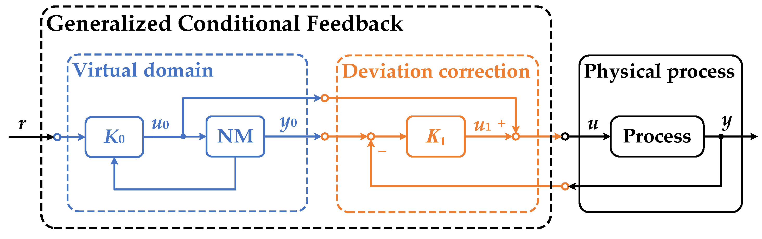
The GCF scheme consists of the virtual domain and the deviation correction part. In the virtual domain, a primary controller is designed to optimize the trajectory of the virtual NM, depicted as,
where K0 denotes the controller designed in the virtual domain, and the constraint set Z0 is a tightened version of the original constraint set (3) such that Z0 ⊆ Z. The tightened constraint is used to ensure performance robustness and is defined in Section 3.3. Assumption 2 guarantees the performance of the controller K0.
In the deviation correction part, another ancillary controller is designed to drive the physical process to track the trajectory of the virtual domain, depicted as,
where K1 denotes the ancillary correction controller, also designed based on the only known NM, and ts is the specified time scale, such that the deviation correction controller efficiently drives the physical process to track the trajectory of the virtual domain. Assumption 1 guarantees that such an ancillary correction controller K1 can be designed.
For additional clarity, the architecture of the proposed GCF control scheme is shown in Figure 1. This diagram highlights the following facts:
- I.
- There are two systems being controlled: the NM (5) is virtual, and the controlled process (1) is physical.
- II.
- In the virtual domain, the trajectory of the virtual NM is optimized to be the desired state of the physical process.
- III.
- The two systems are connected only by the deviation correction controller, which essentially tries to drive the physical process to track the desired trajectory coming from the virtual domain.
Moreover, comprehensive explanations of the GCF scheme are summarized below:
- I.
- The controller in the virtual domain can be any feasible control strategy that is capable of optimizing NM to a specified state.
- II.
- III.
- The stability and the optimization are unified. The controller in the virtual domain ensures optimization and the ancillary correction controller guarantees stability.
3.2. Conditional Feedback
Conditional feedback (CF) is proposed to enable a decoupled input–output response and disturbance–output response [34]. A basic configuration for a linear CF system is shown in Figure 2, where Gp denotes the controlled process, GT denotes the tracking controller, GD denotes the disturbance rejection controller, and r, d, and y are the setpoint, the external disturbances, and the process output, respectively. From the system shown, we learn that the accurate model is needed for CF system design, and the Laplace transform Y of the output y is
which shows that the input–output response is completely determined by the tracking controller GT, and the feedback controller GD acts solely to reject disturbance.
The block diagram of the proposed GCF scheme is similar to that of CF. In the uncertainty-free case where q = {0}, the optimal controller in the virtual domain of GCF can be designed as K0 = GT Gp−1, such that GCF also permits designing an input–output response and disturbance–output response independently. In the view of improving performance robustness, CF can be regarded as an example of GCF acting for inverse system control.
However, their original intentions are different. GCF aims to simultaneously guarantee closed-loop performance and robustness for industrial processes with model uncertainty, while CF focuses on removing conflict between the input–output response and disturbance–output response under the assumption of no model uncertainty. Moreover, CF was proposed based on the classical transfer function method, but GCF is open to the well-developed modern control theory and booming artificial intelligence trend.
3.3. Closed-loop Performance Robustness
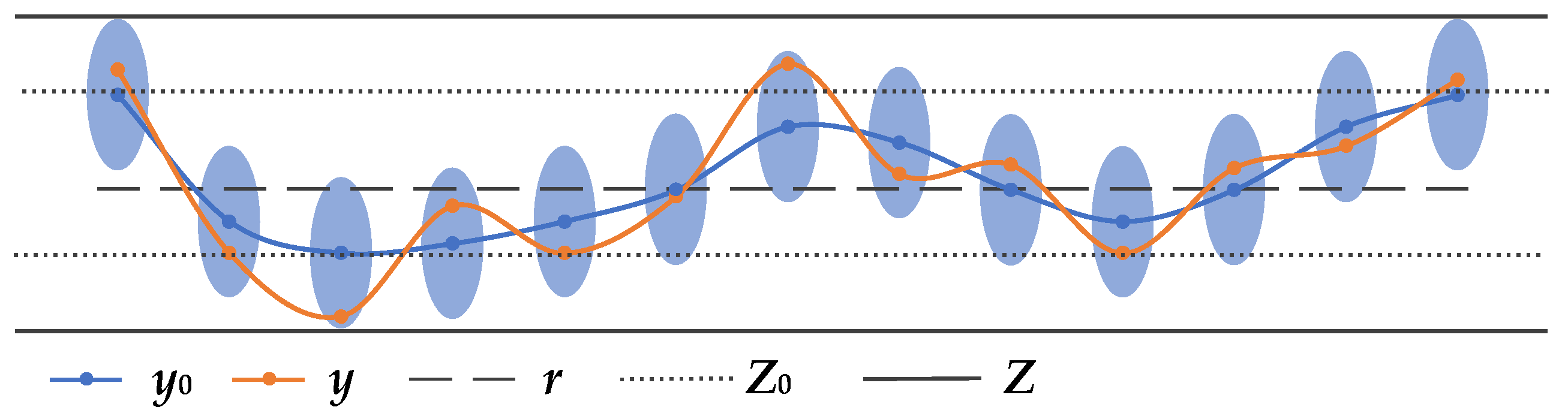
In the context of this work, a property is considered performance robustness if it holds control constraints (3) in the presence of norm-bounded model uncertainty. Recall that the virtual domain optimizes the trajectory of the simulated NM under the constraint z0 ∈ Z0. The deviation correction controller then drives the physical process to track this trajectory. Unfortunately, perfect tracking is impossible because of model uncertainty. Thus, choosing Z0 = Z will not guarantee performance constraint satisfaction for the physical process. In industrial practice, a tightened version of the original constraint (3) is chosen, as represented in Figure 3.
Of particular interest is how we set Z0 to guarantee performance constraint satisfaction. Defining the error δy = y − y0 and δu = u − u0, it follows that
A performance error is defined as
where H(·) is the defined performance error function that denotes the performance variable of the deviation correction controller driving the uncertain process.
Since the considered model is norm-bounded, it follows that
which means the performance error is bounded by the worst-case bound Δz. The value of Δz depends on the performance robustness of the deviation correction controller and model uncertainty. Then, the constraint set Z0 of the virtual domain can be designed as
which is a tightened version of Z. With this tightened performance constraint set, the nominal trajectory optimized by the virtual domain will account for the tracking error and ensure performance constraint satisfaction.
Performance Robustness.
Suppose that the deviation correction controller is performance robust. Then, under the proposed control structure (GCF), the uncertain process (1) will robustly satisfy the performance constraints (3). The closed-loop performance robustness of GCF depends on the performance robustness of the deviation correction controller.
The requirement that the deviation correction controller is performance robust is natural and is satisfied by properly choosing and tuning a non-model-based controller.
3.4. Practice Procedure
The practice procedure of the GCF scheme is now summarized as Algorithm 1. In the online portion, it is suggested that the deviation correction controller is used as a “startup” controller to satisfy basic requirements (e.g., stability, safety). Then, GCF takes over to drive the physical process to guarantee performance constraint satisfaction.
| Algorithm 1: Practice procedure of the GCF scheme. |
| 1: system identification (offline) |
| get a nominal model |
| 2: simulation design (offline) |
| K0 ← Equation (6) |
| K1 ← Equation (7) |
| 3: practice (online) |
| startup control |
| u ← K1 (r, y, u) |
| u0 ← u |
| then |
| u0 ← K0 (r, y0, u0) |
| u1 ← K1 (y, y0, u0, u1) |
| u ← u0 + u1 |
Additionally, when the “startup” controller is applied to the physical process, the virtual domain is in a tracking stage, such that the simulated NM is controlled by
which ensures a reasonable initial condition when the GCF scheme takes control of the physical process.
4. Simulation Illustration
In this section, several model-based control methods are computed as illustrative examples, based on MATLAB R2023a. Please note that PID control tuned by the Skogestad internal model control (SIMC-PID) [35] is selected as the deviation correction controller in all simulation experiments, expressed as
Six typical industrial processes are depicted in Table 1 [27] and three model-based control methods, namely full-state feedback control (FSFC), linear quadratic regulator (LQR), and model prediction control (MPC), are simulated to illustrate the effectiveness of the proposed GCF scheme.
The concern of simulation experiments is the tracking performance robustness. First, norm-bounded model uncertainties of six typical industrial processes in the simulation experiments are assumed in Table 2. All tuned controller parameters are listed in Table 3. In particular, the details of the controller design are explained as follows:
- I.
- State observers are designed when FSFC and LRQ are applied to uncertain models. The observer estimation speed is selected to be 3~5 times the closed-loop response.
- II.
- For processes, G1(s)~G4(s), the state-space models are all expressed as the second controllable canonical form.
- III.
- The pole placements and the cost functions are listed in Table 4.
- IV.

Table 4.
Placed poles and cost functions.
| Control Methods | Processes | Placed Poles | |
|---|---|---|---|
| Closed-Loop | State Observer | ||
| FSFC | G1(s) | [−1+j, −1−j, −1 −2] | [−2+2j, −2−2j, −2 −4] |
| G2(s) | [−7+5j, −7−5j, −10] | [−15+10j, −15−10j, −15] | |
| LQR | G3(s) | Cost function: | [−8+4j, −8−4j] |
| G4(s) | [−10+5j, −10−5j] | ||
Tracking responses and Monte Carlo trials [37] are carried out to quantify the performance robustness of original control methods and GCF schemes. The statistical results are summarized in Table 5. Obviously, the control scheme, designed based on NM, cannot make the uncertain process behave as expected. Nevertheless, the orange part is closer to the red line than the cyanic part, which means the GCF schemes try to buffer the actual response against model uncertainties. Moreover, in the Monte Carlo trials, the performance indices of GCFs are more clustered and closer to zero than those of the original control methods. It also statistically proves the improvement of the performance robustness with the proposed GCF scheme. Consequently, the effectiveness of the proposed GCF scheme is illustrated for model uncertainty.
5. Experiment Validation on a Half-Quadrotor System
The proposed methodology is validated on a half-quadrotor system, whose control has been studied by worldwide researchers [38,39]. LQR is chosen in this section.
5.1. System Model
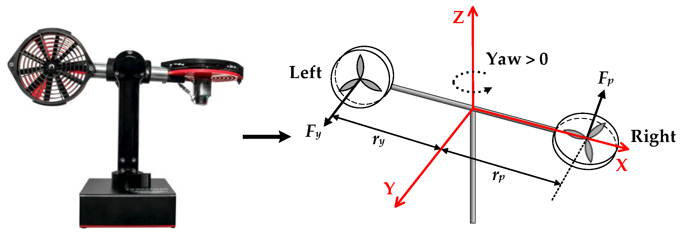
The half-quadrotor system and its free-body diagram are presented in Figure 4. The left propeller is perpendicular to the ground and the right propeller is horizontal. The pitch-axis is locked and only the yaw motion is considered. The yaw angle increases positively, caused by both propellers when the body rotates counter-clockwise about the Z axis.
A simple linear model is developed to represent the motion of the half-quadrotor system about the yaw axis, depicted as
where Jy and Dy are the total moment of inertia and the viscous damping coefficient about the yaw axis, τy is the total torque acting on the yaw axis, Kyp, Kyy, Vp, and Vy are the torque-thrust gain acting on the yaw axis from the right rotor and the left rotor, the voltage applied to the right rotor and the left rotor, respectively. The unmodeled nonlinearity, such as external disturbances and uncertain parameters, is regarded as the model uncertainty.
Voltages with the same magnitude and opposite direction are applied to the two motors. The transfer function between the voltage and the yaw angle is a first-order integral system with inertia, depicted as,
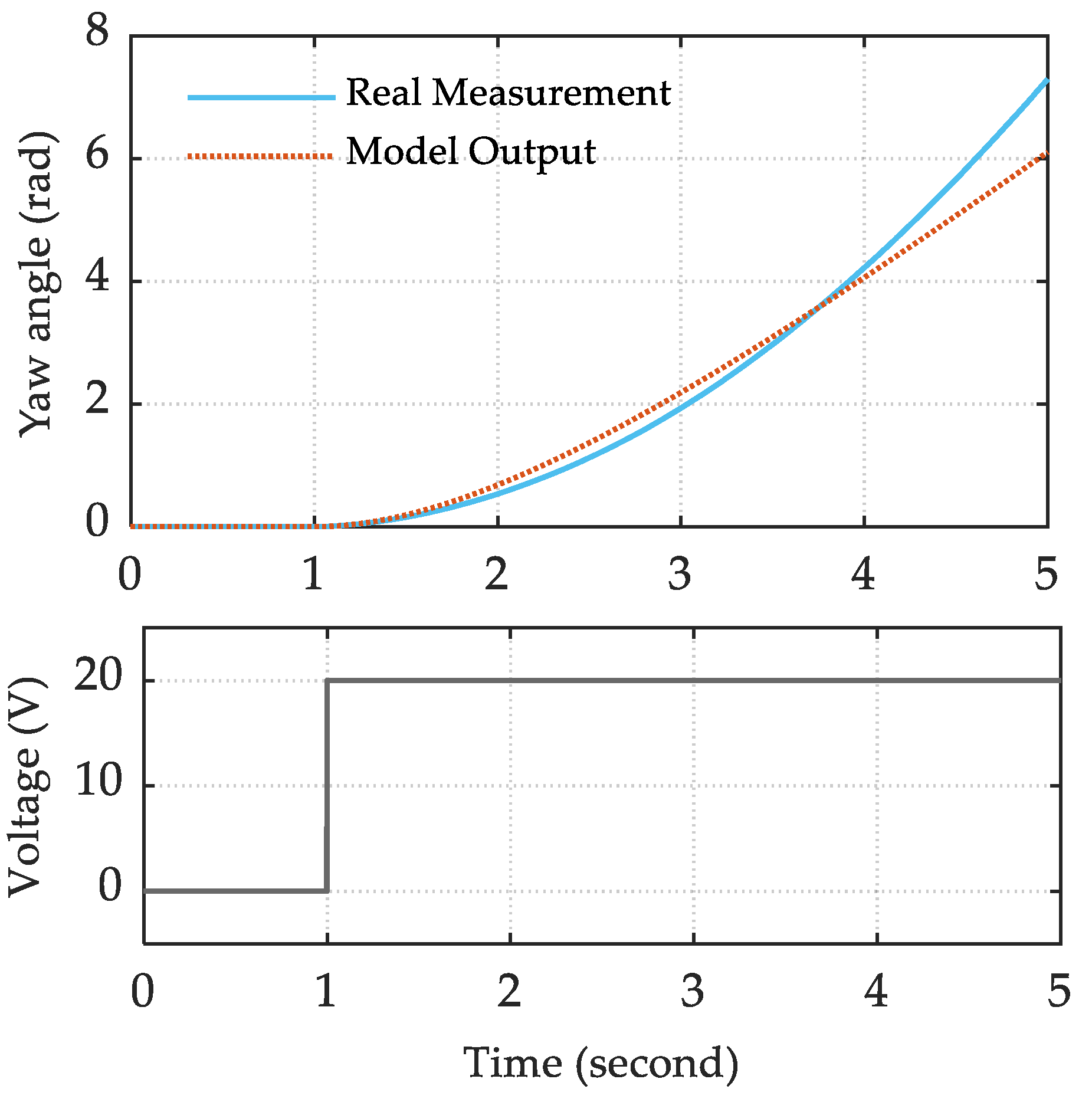
The Quanser Aero Laboratory Guide gives the total moment of inertia, Jy = 0.0220 kg-m2. The viscous damping coefficient, Dy, and the total torque-thrust gain, Kyp + Kyy, are identified by an open-loop step test. In this test, a step voltage of 20 V is added at 1 s, and a genetic algorithm (GA) [40] is used for parameter optimization. Figure 5 shows the results of the identification test. Finally, the transfer function between the voltage and the yaw angle is expressed as
5.2. Control Structure
The half-quadrotor system directly interacts with the PC via a USB link, and the schematic control structure is shown in Figure 6. LQRs and LQR-based GCF schemes are implemented in MATLAB R2021b. Please note that the nominal model (17) is expressed as the second controllable canonical form for LQR design, and the state observer is designed to be a second-order low-pass filter.
5.3. Experiment Results
All control parameters, tuned based on (17), are listed in Table 6. The desired yaw angle is a rectangular wave with an amplitude of 45 deg and a frequency of 0.05 Hz, and the control voltage range is between ±24 V.
The closed-loop response performance is specified as
- Steady-state error: ess ≤ 2 deg.
- Peak time: tp ≤ 3 s.
- Percent Overshoot: PO ≤ 2%.
5.3.1. Experiment 1: Standard System
In this experiment, the half-quadrotor system is standard, as seen in Figure 6. The model uncertainty mainly comes from modeling errors. The experiment results are presented in Figure 7, and the closed-loop response average performance indices are calculated and compared in Figure 10.
From Figure 7 and Figure 10, we can learn that LQR-based GCF has a better closed-loop response than LQR, especially in the steady-state error. Model-based LQR has an intolerable steady-state error, while the GCF scheme satisfies the closed-loop response specifications. In conclusion, the experiment results verify the effectiveness of the proposed GCF scheme preliminarily. In addition, the reason LQR-based GCF (orange line) cannot perfectly track the virtual trajectory (dotted red line) is that the deviation correction controller (PID) behaves conservatively to avoid the control voltage saturation.
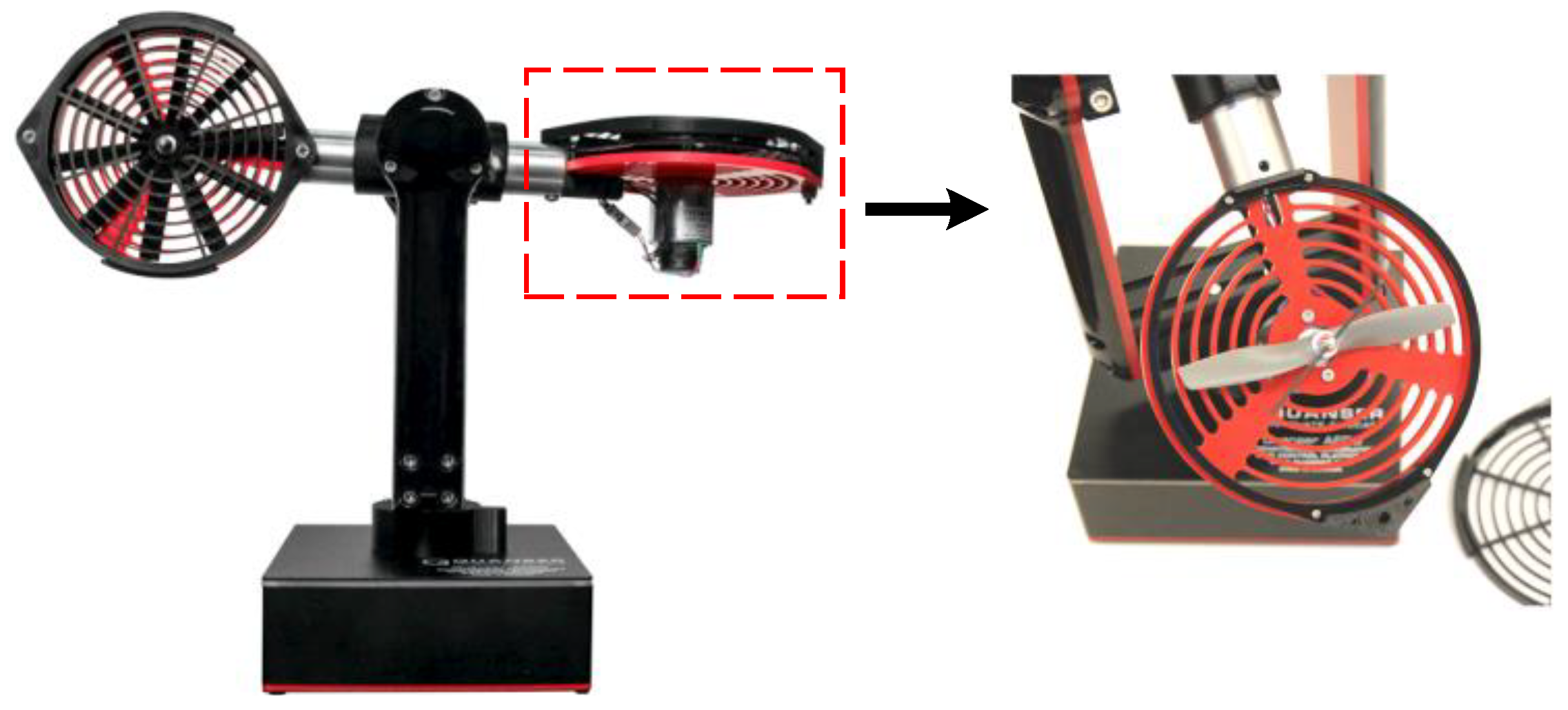
5.3.2. Experiment 2: Changing the Propeller
In this part, we remove the guard cap of the right propeller and insert a small hex key in the right propeller hub to further validate the effectiveness of the proposed GCF scheme, as shown in Figure 8. In this case, the model error is larger, which means there is a larger model uncertainty. This setup is natural and can simulate equipment failure in industrial processes.
The experiment results and average performance indices are presented in Figure 9 and Figure 10. Obviously, for the changed half-quadrotor system, LQR behaves disastrously in the steady-state error. Nevertheless, GCF can still work and achieve satisfactory closed-loop responses. Consequently, the effectiveness of the proposed GCF scheme for model uncertainty is demonstrated.
Figure 9.
Experiment results of the changed half-quadrotor system.
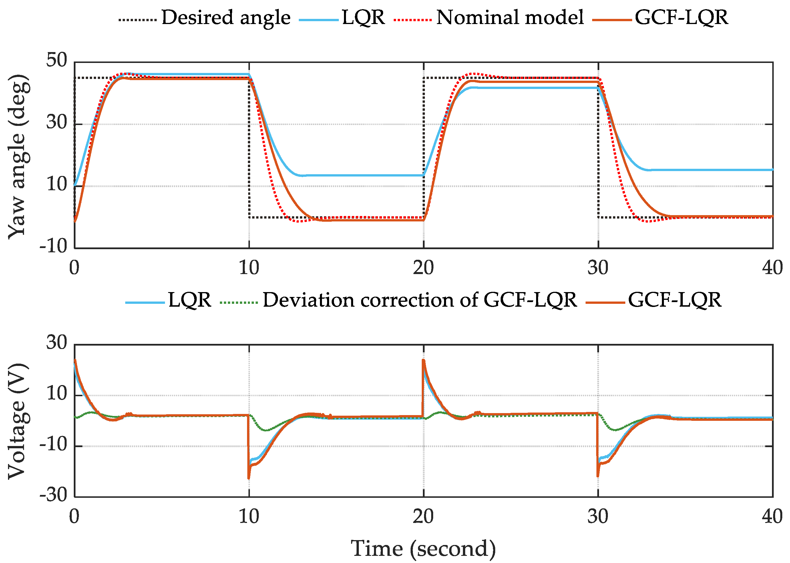
Figure 10.
Closed-loop response average performance indices.
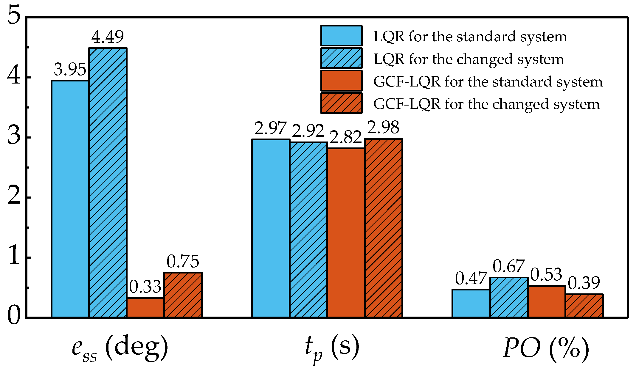
There is, in addition, one further point to make: the half-quadrotor system is insensitive to a low control voltage, which means the system has no integration effect on the low voltage. This causes LQR-based GCF to still have a steady-state error in the presence of an integral correction function.
6. Conclusions
In this article, a GCF scheme is proposed for controlling industrial processes with model uncertainties. Its basic concept and practical implications are elaborated. The approach leverages nominal models and defines an ancillary feedback controller to guarantee closed-loop performance constraints and robustness simultaneously. This scheme is open, such that based on a nominal model, any existing optimal control theory can be designed in the virtual domain, and any robust control algorithm is used as an ancillary feedback controller to drive the physical process to track the trajectory of the virtual domain. The effectiveness of the proposed GCF scheme is validated by numerous case studies and a half-quadrotor system control test.
Future work: There are some additional considerations in terms of both theoretical and practical significance related to this work. First, a further theoretical analysis is necessary. Second, the optimality of an ancillary feedback controller and uncertainty size could be considered. Third, under physical constraints, such as actuator constraints, the limit of the controller in the virtual domain should be considered. Fourth, extensions to reinforcement learning control or digital-twin-enabled smart control are of significant interest.
Author Contributions
Conceptualization, D.L. and C.D.; methodology, D.L. and C.D.; software, C.D.; validation, C.D.; formal analysis, C.D.; investigation, C.D.; resources, C.D.; data curation, C.D.; writing—original draft preparation, C.D.; writing—review and editing, C.D., Z.G., Y.C. and D.L.; visualization, C.D.; supervision, Z.G., Y.C. and D.L.; project administration, D.L.; funding acquisition, D.L. All authors have read and agreed to the published version of the manuscript.
Funding
This research was funded by the Science Center for Gas Turbine Project (P2021-A-I-003-002).
Data Availability Statement
Data are contained within the article.
Conflicts of Interest
The authors declare no conflict of interest.
References
- Degrave, J.; Felici, F.; Buchli, J.; Neunert, M.; Tracey, B.; Carpanese, F.; Ewalds, T.; Hafner, R.; Abdolmaleki, A.; de las Casas, D.; et al. Magnetic control of tokamak plasmas through deep reinforcement learning. Nature 2022, 602, 414–419. [Google Scholar] [CrossRef] [PubMed]
- Tsien, H.S. Engineering Cybernetics; McGraw-Hill: New York, NY, USA, 1954. [Google Scholar]
- Samad, T.; Bauer, M.; Bortoff, S.; Di Cairano, S.; Fagiano, L.; Odgaard, P.F.; Rhinehart, R.R.; Sánchez-Peña, R.; Serbezov, A.; Ankersen, F.; et al. Industry engagement with control research: Perspective and messages. Annu. Rev. Control 2020, 49, 1–14. [Google Scholar] [CrossRef]
- Yedavalli, R.K. Robust Control of Uncertain Dynamic Systems: A Linear State Space Approach; Springer: New York, NY, USA, 2013. [Google Scholar]
- Brockett, R. New Issues in the Mathematics of Control. In Mathematics Unlimited—2001 and Beyond; Engquist, B., Schmid, W., Eds.; Springer Berlin Heidelberg: Berlin/Heidelberg, Germany, 2001; pp. 189–219. [Google Scholar]
- Petersen, I.R.; Ugrinovskii, V.A.; Savkin, A.V. Robust Control Design Using H−∞ Methods; Springer: London, UK, 2000. [Google Scholar]
- Sun, L.; Li, D.H.; Lee, K.Y. Optimal disturbance rejection for PI controller with constraints on relative delay margin. Isa Trans. 2016, 63, 103–111. [Google Scholar] [CrossRef] [PubMed]
- Guo, L. Feedback and uncertainty: Some basic problems and results. Annu. Rev. Control 2020, 49, 27–36. [Google Scholar] [CrossRef]
- Somefun, O.A.; Akingbade, K.; Dahunsi, F. The dilemma of PID tuning. Annu. Rev. Control 2021, 52, 65–74. [Google Scholar] [CrossRef]
- Dorf, R.C.; Bishop, R.H. Modern Control Systems; Pearson Education, Inc.: Hoboken, NJ, USA, 2017. [Google Scholar]
- Anderson, B.D.O.; Moore, J.B. Optimal Control: Linear Quadratic Methods; Prentice-Hall, Inc.: Hoboken, NJ, USA, 1990. [Google Scholar]
- Camacho, E.F.; Bordons, C. Model Predictive Control; Springer London: London, UK, 2007; pp. XXII, 405. [Google Scholar]
- Lorenzetti, J.; McClellan, A.; Farhat, C.; Pavone, M. Linear Reduced-Order Model Predictive Control. IEEE Trans. Autom. Control 2022, 67, 5980–5995. [Google Scholar] [CrossRef]
- Åström, K.J.; Kumar, P.R. Control: A perspective. Automatica 2014, 50, 3–43. [Google Scholar] [CrossRef]
- Åström, K.J.; Wittenmark, B. On self tuning regulators. Automatica 1973, 9, 185–199. [Google Scholar] [CrossRef]
- Kalman, R.E. Design of a Self-Optimizing Control System. Trans. Am. Soc. Mech. Eng. 2022, 80, 468–477. [Google Scholar] [CrossRef]
- Morse, A.S. Global Stability of Parameter-Adaptive Control Systems. IEEE Trans. Autom. Control 1980, 25, 433–439. [Google Scholar] [CrossRef]
- Doyle, J.C.; Glover, K.; Khargonekar, P.P.; Francis, B.A. State-space solutions to standard H-2 and H-∞ control-problems. IEEE Trans. Autom. Control 1989, 34, 831–847. [Google Scholar] [CrossRef]
- Packard, A.; Doyle, J. The complex structured singular value. Automatica 1993, 29, 71–109. [Google Scholar] [CrossRef]
- Zames, G. Feedback and optimal sensitivity-model-reference transformations, multiplication seminorms, and approximate inverses. IEEE Trans. Autom. Control 1981, 26, 301–320. [Google Scholar] [CrossRef]
- Annaswamy, A.M.; Fradkov, A.L. A historical perspective of adaptive control and learning. Annu. Rev. Control 2021, 52, 18–41. [Google Scholar] [CrossRef]
- Rohrs, C.E.; Valavani, L.; Athans, M.; Stein, G. Robustness of continuous-time adaptive-control algorithms in the presence of unmodeled dynamics. IEEE Trans. Autom. Control 1985, 30, 881–889. [Google Scholar] [CrossRef]
- Glover, K.; Limebeer, D.J.N.; Doyle, J.C.; Kasenally, E.M.; Safonov, M.G. A characterization of all solutions to the 4 block general distance problem. Siam J. Control Optim. 1991, 29, 283–324. [Google Scholar] [CrossRef]
- Safonov, M.G. Origins of robust control: Early history and future speculations. Annu. Rev. Control 2012, 36, 173–181. [Google Scholar] [CrossRef]
- Wang, C.; Li, D. Decentralized PID Controllers Based on Probabilistic Robustness. J. Dyn. Syst. Meas. Control-Trans. Asme 2011, 133, 061015. [Google Scholar] [CrossRef]
- Wang, F.C. Research on PID Control for Thermal Process Based on Probabilistic Robustness. J. Dyn. Sys. Meas. Control 2008, 133, 061015. [Google Scholar] [CrossRef]
- Wu, Z. Robust Active Disturbance Rejection Control Design for Thermal System; Tsinghua University: Beijing, China, 2020. [Google Scholar]
- Xu, F. Research on Robust PID Controller and Its Applications in Control of Thermal Plants. Master’s Thesis, Tsinghua University, Beijing, China, 2002. [Google Scholar]
- Liu, K.; Tiao, Y. Linear Robust Control; Science Press: Beijing, China, 2013. [Google Scholar]
- Zhang, W. Quantitative Process Control Theory; Routledge: Abingdon, UK, 2011; pp. 1–439. [Google Scholar]
- Huba, M.; Bistak, P.; Vrancic, D. Series PIDA Controller Design for IPDT Processes. Appl. Sci. 2023, 13, 2040. [Google Scholar] [CrossRef]
- Wang, W.; Li, D.; Xue, Y. Decentralized Two Degree of Freedom PID Tuning Method for MIMO processes. In Proceedings of the IEEE International Symposium on Industrial Electronics (ISIE 2009), Seoul, Republic of Korea, 5–8 July 2009; pp. 143–148. [Google Scholar]
- Han, J. From PID to Active Disturbance Rejection Control. IEEE Trans. Ind. Electron. 2009, 56, 900–906. [Google Scholar] [CrossRef]
- Lang, G.; Ham, J.M. Conditional Feedback Systems—A New Approach to Feedback Control. Trans. Am. Inst. Electr. Eng. Part II Appl. Ind. 1955, 74, 152–161. [Google Scholar] [CrossRef]
- Skogestad, S. Simple analytic rules for model reduction and PID controller tuning. J. Process Control 2003, 13, 291–309. [Google Scholar] [CrossRef]
- Normey-Rico, J.E.; Camacho, E.F. Dead-time compensators: A survey. Control Eng. Pract. 2008, 16, 407–428. [Google Scholar] [CrossRef]
- Liu, S.; Zhang, Y.-L.; Xue, W.; Shi, G.; Zhu, M.; Li, D. Frequency response-based decoupling tuning for feedforward compensation ADRC of distributed parameter systems. Control Eng. Pract. 2022, 126, 105265. [Google Scholar] [CrossRef]
- Khanesar, M.A.; Kayacan, E. Controlling the Pitch and Yaw Angles of a 2-DOF Helicopter Using Interval Type-2 Fuzzy Neural Networks. In Recent Advances in Sliding Modes: From Control to Intelligent Mechatronics; Yu, X., Önder Efe, M., Eds.; Springer International Publishing: Cham, Switzerland, 2015; pp. 349–370. [Google Scholar]
- Nettari, Y.; Labbadi, M.; Kurt, S. Adaptive Backstepping Integral Sliding Mode Control Combined with Super-Twisting Algorithm For Nonlinear UAV Quadrotor System. IFAC-Pap. 2022, 55, 264–269. [Google Scholar] [CrossRef]
- Sivanandam, S.N.; Deepa, S.N. Introduction to Genetic Algorithms; Springer: Berlin, Germany, 2008. [Google Scholar]
Figure 1.
Block diagram of the proposed GCF scheme, which shows the connection between the virtual NM (5) and the controlled process (1).
Figure 1.
Block diagram of the proposed GCF scheme, which shows the connection between the virtual NM (5) and the controlled process (1).

Figure 2.
The basic configuration of a linear conditional feedback system.
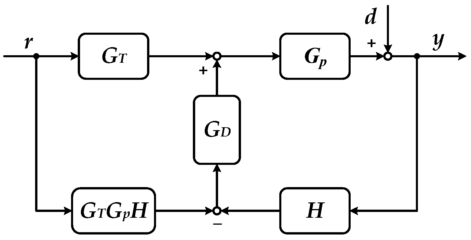
Figure 3.
Performance constraint satisfaction using tightened constraints in the virtual domain.

Figure 4.
Half-quadrotor system and its free-body diagram.

Figure 5.
Results of the identification test.

Figure 6.
The schematic control structure of the half-quadrotor system.
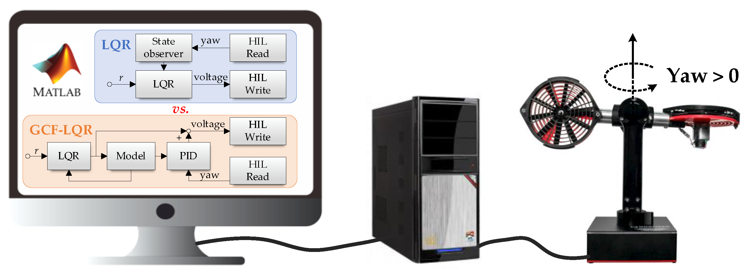
Figure 7.
Experiment results of the standard half-quadrotor system.
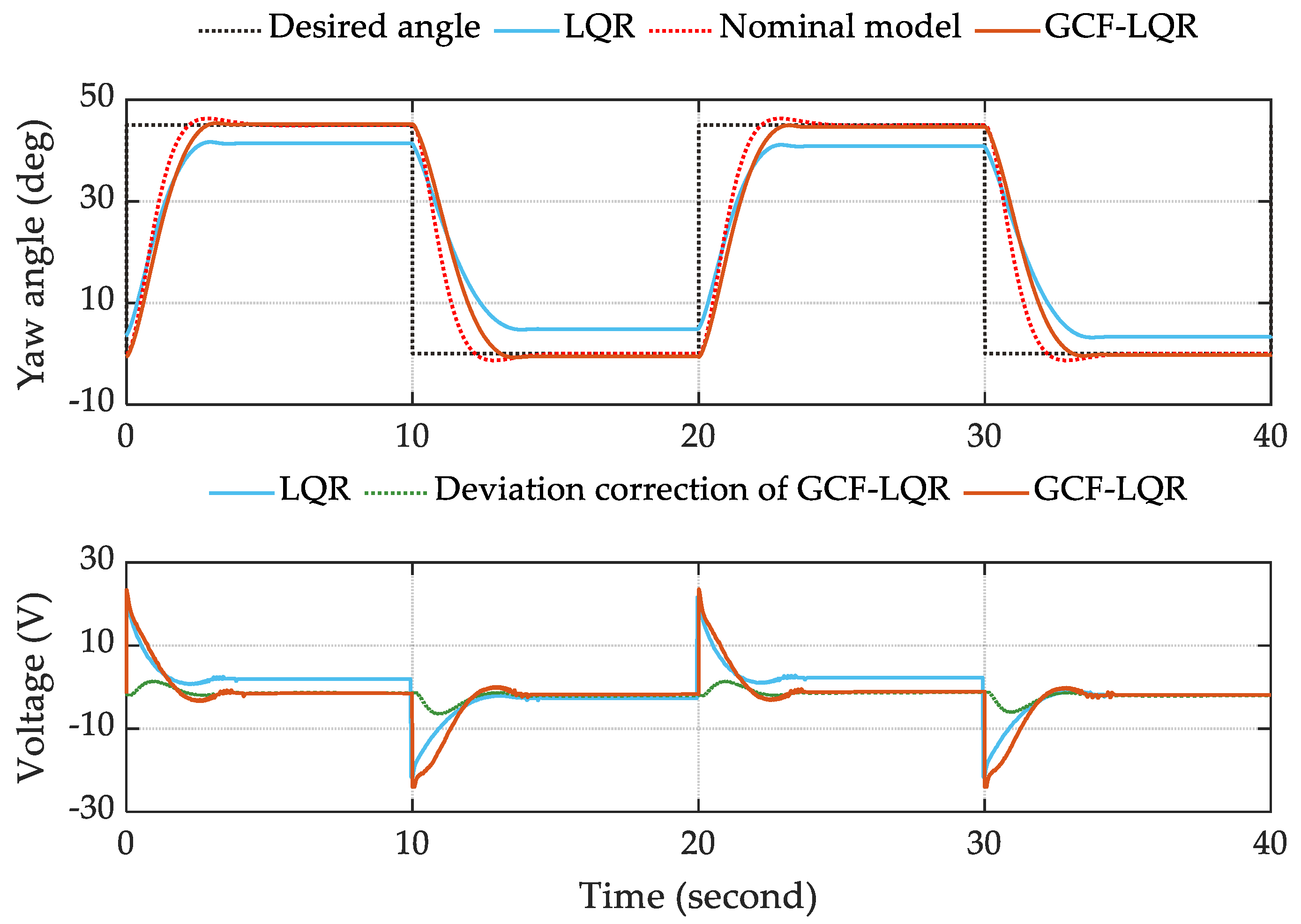
Figure 8.
Diagram of changing the right propeller.

Table 1.
Six typical industrial processes as a benchmark test set.
| Process Types | Process Models |
|---|---|
| High-order process | |
| Integral process | |
| Low-order process | |
| Unstable process | |
| Time-delay process | |
| Nonminimum-phase process |
Table 2.
Model uncertainties of six typical industrial processes, where the model uncertainty matrix denotes the limit of model parameters varying near nominal values defined in Table 1, i.e., Δa1 denotes a1∈[a10 − Δa1, a10 + Δa1], where a10 is the nominal value of a1 in Table 1.
| Process Models | Model Uncertainties [Δa1 Δa2, …] |
|---|---|
| [0.25 0.25 0.25 0.25] | |
| [0.25 1.5 3] | |
| [1 1 1] | |
| [0.25 0.25] | |
| [0.5 2.5 1 0.5] | |
| [0.5 0.4] |
Table 3.
Tuned controller parameters.
| Control Methods | Processes | Parameters | ||
|---|---|---|---|---|
| Virtual Domain | {Kp, Ki, Kd} | State Observer | ||
| FSFC | G1(s) | [3 6 4 1] | {5/6, 1/3, 0.5} | [6 10 0 −21] |
| G2(s) | [740 142 6] | {1404, 2592, 180} | [27 217 −975] | |
| LQR | G3(s) | [13.1774 2.8879] | {5.5, 55/8, 0} | [10 15] |
| G4(s) | [14.1421 7.2677] | {12.5, 4.8, 7.8} | [21 146] | |
| MPC | G5(s) | Ts = 0.2 s, p = 50, m = 2 | {12.5, 1.25, 20} | - |
| G6(s) | Ts = 0.1 s, p = 50, m = 2 | {0.5, 0.2, 0.3} | - | |
Table 5.
Statistical results of the tracking response and the Monte Carlo trial, where the dotted black line is the setpoint, the dotted red line is the closed-loop response of the nominal model, the orange part represents GCF, and the cyanic part represents the original control method.
Table 5.
Statistical results of the tracking response and the Monte Carlo trial, where the dotted black line is the setpoint, the dotted red line is the closed-loop response of the nominal model, the orange part represents GCF, and the cyanic part represents the original control method.
| Processes | Tracking Responses (N = 100) | Monte Carlo Trials (N = 1000) |
|---|---|---|
| G1(s) | 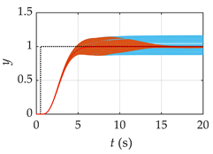 |  |
| G2(s) | 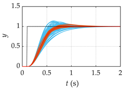 | 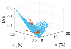 |
| G3(s) | 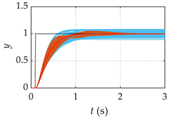 | 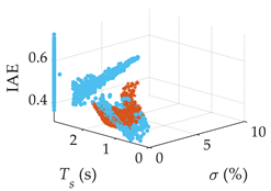 |
| G4(s) |  | 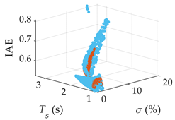 |
| G5(s) |  | 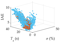 |
| G6(s) | 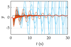 | 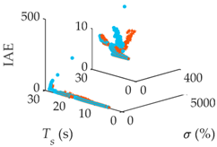 |
Please note that the indices {δ, Ts, IAE} are the relative overshoot, the settling time (2% criterion), and the absolute error integral, respectively.
Table 6.
Tuned controller parameters.
| Control Schemes | Parameters | |
|---|---|---|
| LQR | ωc = 45, ξ = 0.8 | Q = diag ([100 0]), R = 0.1 K = [31.6228 19.2195] |
| GCF-LQR | Kp = 8.5, Ki = 2.0, Kd = 6.4 | |
Please note that the ωc and ξ are the cut-off frequency (rad/s) and the damping ratio of the second-order low-pass filter, respectively.
Disclaimer/Publisher’s Note: The statements, opinions and data contained in all publications are solely those of the individual author(s) and contributor(s) and not of MDPI and/or the editor(s). MDPI and/or the editor(s) disclaim responsibility for any injury to people or property resulting from any ideas, methods, instructions or products referred to in the content. |
© 2023 by the authors. Licensee MDPI, Basel, Switzerland. This article is an open access article distributed under the terms and conditions of the Creative Commons Attribution (CC BY) license (https://creativecommons.org/licenses/by/4.0/).
Share and Cite
MDPI and ACS Style
Dai, C.; Gao, Z.; Chen, Y.; Li, D. Generalized Conditional Feedback System with Model Uncertainty. Processes 2024, 12, 65. https://doi.org/10.3390/pr12010065
AMA Style
Dai C, Gao Z, Chen Y, Li D. Generalized Conditional Feedback System with Model Uncertainty. Processes. 2024; 12(1):65. https://doi.org/10.3390/pr12010065
Chicago/Turabian StyleDai, Chengbo, Zhiqiang Gao, Yangquan Chen, and Donghai Li. 2024. "Generalized Conditional Feedback System with Model Uncertainty" Processes 12, no. 1: 65. https://doi.org/10.3390/pr12010065
Note that from the first issue of 2016, this journal uses article numbers instead of page numbers. See further details here.