Flexible Extension of the Lomax Distribution for Asymmetric Data under Different Failure Rate Profiles: Characteristics with Applications for Failure Modeling and Service Times for Aircraft Windshields

Abstract

A novel four-parameter lifetime Lomax model is presented and investigated within the scope of this paper. The failure rate of the innovative model can be “monotonically decreasing failure rate,” “monotonically increasing failure rate,” or “constant failure rate,” and the density of the model can be “asymmetric right skewed,” “symmetric,” “asymmetric left skewed,” or “uniform density”. The new density is expressed as a blend of the Lomax densities that have been multiplied by an exponent. New bivariate Lomax types were created for our research. The maximum likelihood technique was utilized. We performed simulated experiments for the purpose of evaluating the finite sample behavior of maximum likelihood estimators, using “biases” and “mean squared errors” as our primary metrics of analysis. The novel distribution was evaluated based on a number of pertinent Lomax models, including Lomax extensions that were generated on the basis of odd log-logistic, Kumaraswamy, beta, gamma, and Topp–Leone families, among others. The newly developed extension demonstrated its relevance by predicting the service and failure times of datasets pertaining to aircraft windshields.

1. Introduction

Probability distributions are important in the field of statistics because they offer a wealth of materials to a variety of statistical subfields. The methods and applications of statistical modeling that are founded on actual data and are utilized in fields such as insurance, actuarial sciences, engineering, dependability, agriculture, and industry, amongst other sectors, are some of the most important aspects of these factors. Probability-based distributions known as heavy-tailed distributions feature probability tails that are more weighted than those observed in the normal distribution. This suggests that they have a greater potential of witnessing values that deviate significantly from the norm (also known as “outliers”) than the normal distribution would indicate for them to have. In contrast, there is a low possibility of discovering extreme values in distributions with light tails, like a normal distribution. The Lomax (Lx) distribution is the most important heavy-tailed probability-based distribution in the field of mathematical modeling. The distribution of wealth and income can be modelled with the help of this distribution, which features an extended tail on the right side of the distribution. Heavy-tailed distributions are essential in a wide variety of fields, including finance, economics, physics, and engineering, due to the fact that they more accurately reflect the phenomena that occur in real life. This is because real-life phenomena are characterized by the occurrence of extreme events more frequently than would be predicted by a normal distribution. It is common practice to employ the Lx distribution for modeling datasets with heavy tails, which means that extreme circumstances occur more frequently than one might assume. The scale and location of the dispersion are the two parameters that make up the Lx. According to TadiKamalla [1] and Corbellini et al. [2], this distribution is commonly employed in the financial and insurance industries to imitate severe occurrences, such as substantial insurance claims or stock market crashes.

The Lx (Pareto type II) distribution is commonly used in actuarial science due to its ability to model heavy-tailed data. This distribution is also known as the Lx distribution or the Pareto distribution of the second kind. It is a continuous probability distribution that is widely used to model the frequency and severity of rare events, such as large insurance claims or natural disasters.

The main goal of this article is to provide and apply a new flexible extension of the Lx distribution called the generalized odd-generalized exponential Lomax (GOGELx) model, which was derived using the generalized odd-generalized exponential-G (GOGE-G) family defined by Alizadeh et al. [3]. A random variable (rv) $Z$ has an Lx distribution if it has a cumulative distribution function (CDF) (for $Z>0$) given by

$$G_{\tau ,\sigma }\left(\mathcal{z}\right){|}_{\left(\tau >0 \mathrm{and} \sigma >0\right)}=1-{\left({\sigma }^{-1}\mathcal{z}+1\right)}^{-\tau },$$

(1)

where $\tau$ and $\sigma$ are the shape and scale parameters, respectively. Then, the corresponding probability density function (PDF) of (1) can be derived as

$$g_{\tau ,\sigma }\left(\mathcal{z}\right)=\frac{\tau }{\sigma }{\left({\sigma }^{-1}\mathcal{z}+1\right)}^{-\left(\tau +1\right)}.$$

(2)

The Lx distribution is particularly useful for analyzing the upper tail of a dataset, where extreme events or outliers are more likely to occur. The Lx distribution is a valuable tool for analyzing extreme events and tail behavior in big data within the transportation domain. By utilizing this distribution, transportation planners can gain insights into rare but impactful events, enabling them to make informed decisions and develop effective strategies to improve system performance, safety, and resilience (see Schumann et al. [4] for more details). In transportation, it can be applied to various scenarios, such as:

I.

The Lx distribution can be used to model the occurrence of severe traffic congestion events. By fitting the distribution to historical data on congestion levels or travel times, transportation planners can estimate the probability of extreme congestion events. This information helps in designing appropriate mitigation strategies and optimizing traffic management plans.

II.

The Lx distribution can be utilized to model the occurrence of rare but severe accidents. By analyzing historical accident data, transportation agencies can estimate the probability of extreme accident events, which aids in prioritizing safety interventions and allocating resources effectively.

III.

In transportation systems, extreme weather events can significantly affect operations and safety. The Lx distribution can be applied to model the occurrence of extreme weather phenomena, such as heavy rainfall, snowstorms, or high winds. By understanding the tail behavior of these events, transportation planners can develop strategies to minimize the impact of adverse weather conditions.

IV.

When analyzing transportation demand, the Lx distribution can be used to model the tail behavior of high-demand events. This is particularly relevant for scenarios in which sudden spikes in demand occur, such as during major events, holidays, or rush hours. By incorporating the Lx distribution into demand forecasting models, transportation planners can estimate the probability of extreme demand levels and ensure appropriate resource allocation.

V.

The Lx distribution can aid in analyzing the tail behavior of traffic or transportation infrastructure capacity. By fitting the distribution to the data on infrastructure utilization, transportation planners can estimate the probability of extreme capacity constraints. This information is valuable for designing infrastructure expansion projects or optimizing capacity allocation strategies.

The CDF and the PDF of the GOGELx model provided by Alizadeh et al. [3], respectively, are as follows:

$$F_{\underset{\_}{V}}\left(\mathcal{z}\right)={\left(1-\mathit{exp}\left\{\mathcal{W}\left(\mathcal{z};a,\tau ,\sigma \right)\right\}\right)}^b{|}_{\left(\underset{\_}{V}=a,b,\tau ,\sigma \right)},$$

(3)

where $\mathcal{W}\left(\mathcal{z};a,\tau ,\sigma \right)=\frac{-{\left[1-{\left({\sigma }^{-1}\mathcal{z}+1\right)}^{-\tau }\right]}^a}{1-{\left[1-{\left({\sigma }^{-1}\mathcal{z}+1\right)}^{-\tau }\right]}^a}$ and

$$f_{\underset{\_}{V}}\left(\mathcal{z}\right)=ab\frac{\tau }{\sigma }\frac{{\left[1-{\left({\sigma }^{-1}\mathcal{z}+1\right)}^{-\tau }\right]}^{a-1}\mathit{exp}\left\{\mathcal{W}\left(\mathcal{z};a,\tau ,\sigma \right)\right\}}{{\left\{1-{\left[1-{\left({\sigma }^{-1}\mathcal{z}+1\right)}^{-\tau }\right]}^a\right\}}^2{\left({\sigma }^{-1}\mathcal{z}+1\right)}^{\left(\tau +1\right)}}{\left[1-\mathit{exp}\left\{\mathcal{W}\left(\mathcal{z};a,\tau ,\sigma \right)\right\}\right]}^{b-1},$$

(4)

where $a,b>0$ are two additional shape parameters. Henceforth, $Z\sim$ GOGELx($\underset{\_}{V}$) denotes a random variable with a density function (4). The reliability function (rf) and hazard rate function (HRF) of $\hspace{0.33em}Z$ are expressed by $h(\mathcal{z})=f_{\underset{\_}{V}}\left(\mathcal{z}\right)/R_{\underset{\_}{V}}\left(\mathcal{z}\right)$, where $R_{\underset{\_}{V}}\left(\mathcal{z}\right)=1-F_{\underset{\_}{V}}\left(\mathcal{z}\right).$ For the purpose of simulating data from this new model, if $u\sim u(0,1)$, then

$${\mathcal{z}}_u=\sigma \left({\left\{1-{\left[\frac{-\mathit{log}\left(1-u^{\frac{1}{b}}\right)}{1-\mathit{log}\left(1-u^{\frac{1}{b}}\right)}\right]}^{\frac{1}{a}}\right\}}^{-\frac{1}{\tau }}-1\right)$$

has CDF in (3). In fact, the specialist literature contains a significant number of extensions of the Lx distribution. These extensions were mostly utilized in the mathematical and statistical modeling procedures, and we will highlight some of them here: the Lx-inverse-Weibull model by Afify et al. [5], a new generalized Lx model with statistical properties and applications by Ibrahim and Yousof [6], a new extension of the Lx distribution by Elbiely and Yousof [7], validation of the Topp–Leone-Lx model by Yadav et al. [8], and a new Lx distribution for modeling survival times and tax revenue datasets by Elsayed and Yousof [9]. In order to show the wide flexibility of the new model, we have presented Figure 1. The new PDF can be “right skewed” with a large tail shape or “right skewed” with one peak, as shown in Figure 1 (the left plot). Either of these two possibilities corresponds to a “right skewed” distribution. As illustrated in Figure 1 (the right plot), the HRF of the GOGELx model can be one of four different types: “decreasing-constant HRF,” “monotonically increasing HRF,” “bathtub HRF,” and “constant HRF”.

When modeling data with two or more variables, an essential piece of statistical software known as a copula is utilized in the process. This function creates a relationship between the marginal distributions of two or more variables and the joint distribution of all variables. The marginal distributions of the variables may be independent or dependent on one another. In recent years, copulas have witnessed a rise in popularity as a result of their adaptability as well as their capacity to model complex dependence patterns between variables. This growth in popularity can be attributed to the fact that copulas are capable of modeling intricate dependency patterns between variables. The capacity of copulas to depict intricate dependency patterns between variables is likely responsible for this meteoric rise in popularity. In this investigation, we generate some new bivariate type GOGELx (BGOGELx) models by employing the Farlie–Gumbel–Morgenstern (FGM) copula, the modified Farlie–Gumbel–Morgenstern (MFGM) copula, the Clayton copula, and Renyi’s entropy (for additional information, see Farlie [10], Morgenstern [11] and Gumbel [12,13]). Customers also have the option to buy a product of a type known as Multivariate GOGELx (MvGOGELx). On the other hand, it is not out of the question that further efforts will be made to research these original ideas. Let us start by looking at the combined CDF of the FGM family, which is made up of the following parts:

$${\mathcal{F}}_{\mathcal{p}}(\mathcal{v}\left(.\right),\mathcal{u}\left(.\right))=\mathcal{v}\left(.\right)\mathcal{u}\left(.\right)\left(1+\mathcal{p}{\mathcal{v}}^{•}\left(.\right){\mathcal{u}}^{•}\left(.\right)\right)$$

where ${\mathcal{v}}^{•}\left(.\right)=1-\mathcal{v}\left(.\right),$ ${\mathcal{u}}^{•}\left(.\right)=1-\mathcal{u}\left(.\right)$ and the marginal function $\mathcal{v}=F_1=F_{{\underset{\_}{V}}_1}\left({\mathcal{z}}_1\right)$, $\mathcal{u}=F_2=F_{{\underset{\_}{V}}_2}\left({\mathcal{z}}_2\right)$, and $\mathcal{p}\in \left(-1,1\right)$ are the dependence parameters, and for every $\mathcal{v}\left(.\right),\mathcal{u}\left(.\right)\in \left(\mathrm{0,1}\right)$, $\mathcal{F}(\mathcal{v}\left(.\right),0)=\mathcal{F}(0,\mathcal{u}\left(.\right))=0$, which is “grounded minimum”, $\mathcal{F}(\mathcal{v}\left(.\right),1)=\mathcal{v}$, and $\mathcal{F}(1,\mathcal{u}\left(.\right))=\mathcal{u}$, which is “grounded maximum”,

$$\mathcal{F}\left({\mathcal{v}}_1\left(.\right),{\mathcal{u}}_1\left(.\right)\right)+\mathcal{F}\left({\mathcal{v}}_2\left(.\right),{\mathcal{u}}_2\left(.\right)\right)-\mathcal{F}\left({\mathcal{v}}_1\left(.\right),{\mathcal{u}}_2\left(.\right)\right)-\mathcal{F}\left({\mathcal{v}}_2\left(.\right),{\mathcal{u}}_1\left(.\right)\right)\ge 0,$$

For more details, see Nelsen (1999). The development of a new GOGELx model did not become a motivated task in and of itself; hence, it is important to provide some convincing arguments and practical considerations that highlight the importance, adaptability, and application of this distribution. In order to accomplish this goal, it is required to present a number of compelling reasons and practical considerations that highlight the significance, adaptability, and usefulness of this distribution. The new PDF elasticity and the HRF that went along with it were both developed as a direct result of these external factors and forces, which served as the driving forces behind their development. When presenting a novel distribution, one of the most important practical aspects that should be taken into account is the possibility of applying it to statistical modeling. In the following scenarios, the GOGELx model may prove to be helpful:

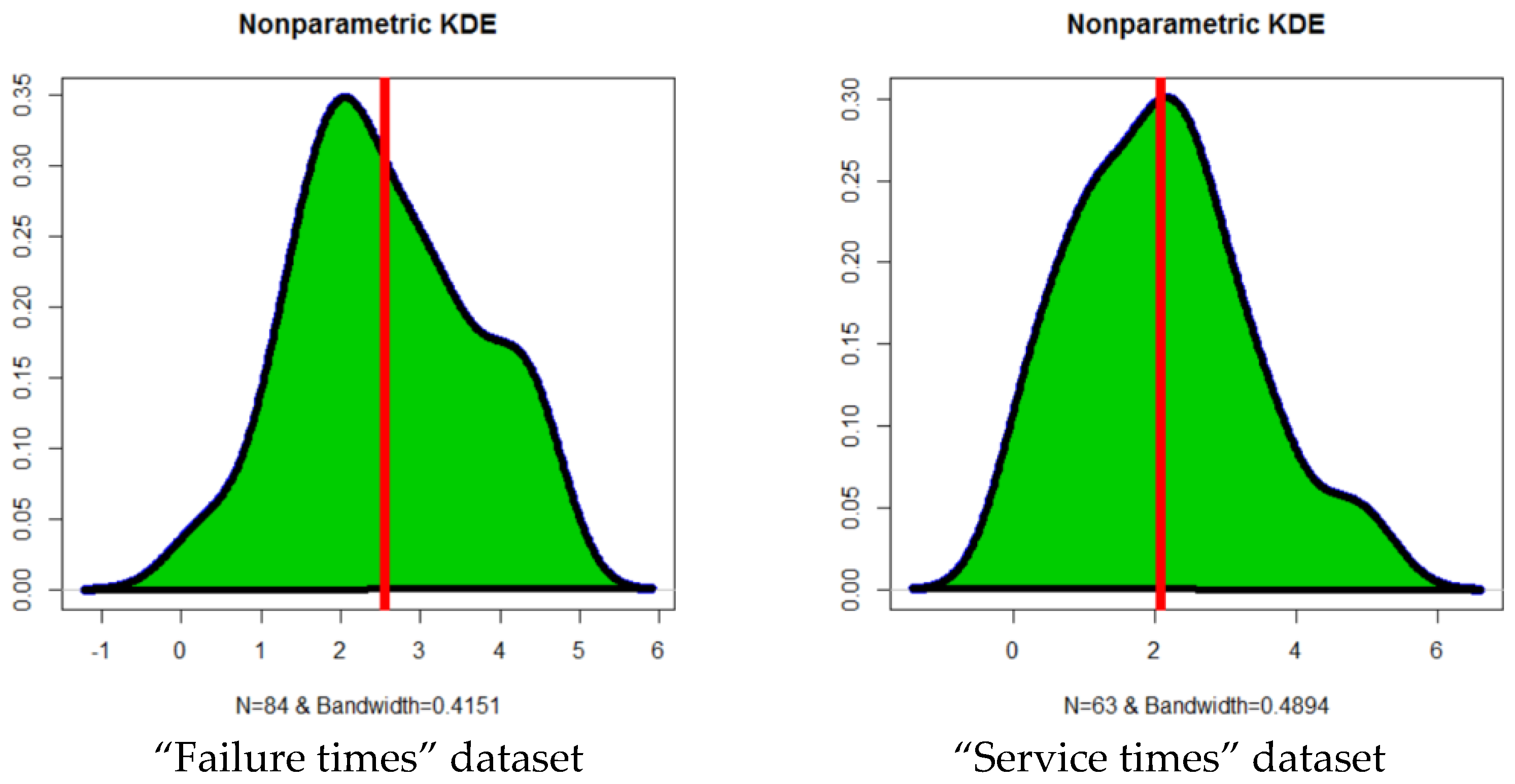
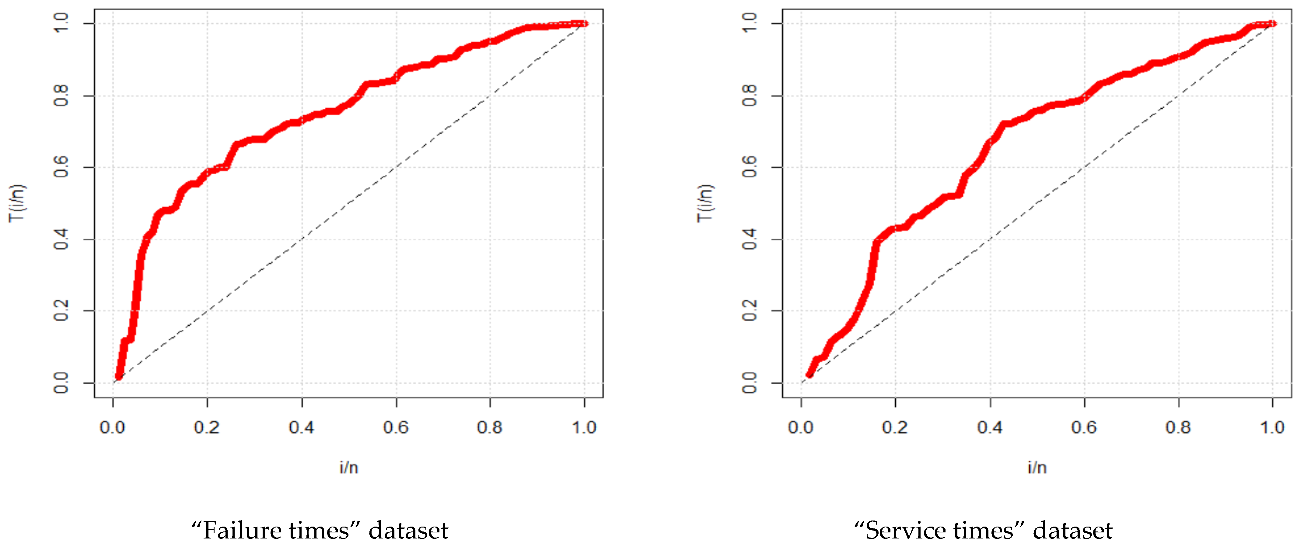
• The real datasets whose kernel density is semi-symmetric (slightly skewed to the left and slightly skewed to the left) and have a bimodal form, as illustrated in Figure 3, are the ones that are discussed here.
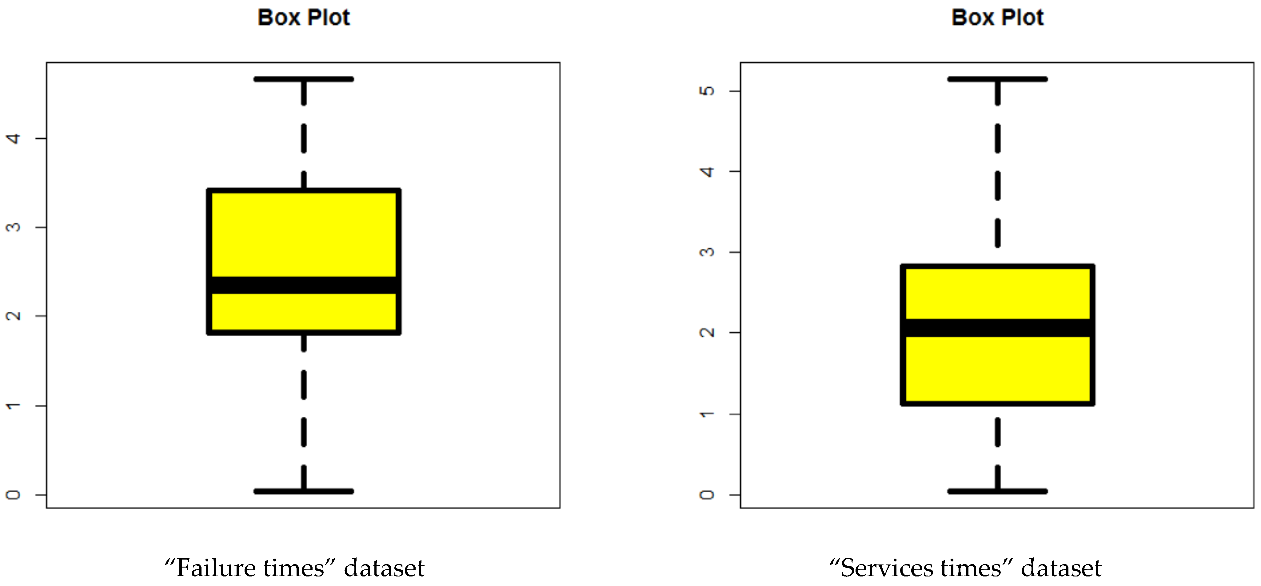
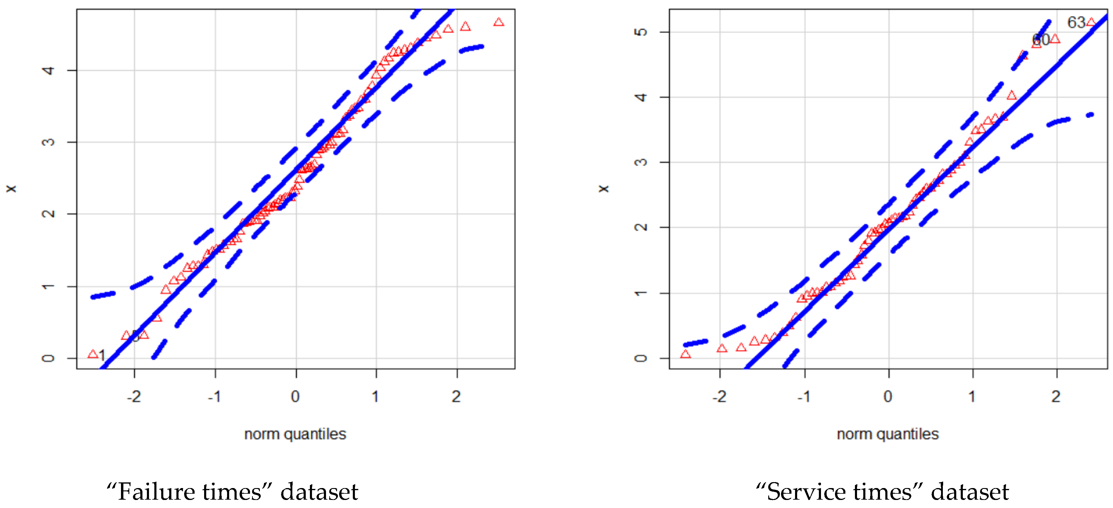
• The real-life datasets, which, as shown in the application Section, do not contain any observations that fall into the extreme category.
• The GOGELx model is compared to many relevant models, such as the special generalized mixture Lx distribution, the Kumaraswamy Lx distribution, beta Lx distribution, gamma Lx distribution, Transmuted Topp–Leone Lx distribution, reduced Transmuted Topp–Leone Lx distribution, odd log-logistic Lx distribution, reduced odd log-logistic Lx distribution, reduced Burr–Hatke Lx distribution, exponentiated Lx distribution, standard Lx distribution, reduced GOGELx distribution, and proportional reversed hazard rate Lx distribution in modeling the failure times of aircraft windshield data.
• The GOGELx distribution is compared to many relevant models, such as the odd log-logistic Lx distribution, the Kumaraswamy Lx distribution, the special generalized mixture Lx distribution, beta Lx distribution, gamma Lx distribution, Transmuted Topp–Leone Lx distribution, reduced Transmuted Topp–Leone Lx distribution, reduced odd log-logistic Lx distribution, reduced Burr–Hatke Lx distribution, exponentiated Lx distribution, standard Lx distribution, reduced GOGELx distribution, and proportional reversed hazard rate Lx distribution in modeling the service times of aircraft windshield data.
• Creating new probability density functions that may take on several beneficial forms, such as “right skewed” with a heavy tail shape and “right skewed” with one peak.
• Any new model may be used to analyze a variety of environmental datasets because of the great flexibility of the probability density function. But the new model has shown flexibility and high efficiency in the statistical and mathematical modeling processes of different sets of reliability and engineering data.
• Introducing a few new one-of-a-kind models that come with a variety of hazard rate functions, such as “decreasing constant HRF,” “monotonically increasing HRF,” “bathtub HRF,” and “constant HRF.” The number of distinct failure rate categories has a positive correlation with the elasticity of the distribution. These forms make the work of a wide variety of practitioners, including those who would use the new distribution in statistical modeling and mathematical analysis, significantly simpler. The matter of checking the success rate function for this particular endeavor has received a significant amount of focus and consideration from our team.
• The degree to which the new distribution is flexible can be determined, in part, by looking at the skew coefficient, the kurtosis coefficient, the failure rate function, and the variety of the PDF and failure rate functions. In this context, it is of the utmost importance to give some thought to the accuracy with which the probability distribution may be modeled statistically, as well as the accuracy with which it can be employed. As a direct consequence of this, we examined the probability distribution in great detail. It is essential to emphasize in this piece that the new family has distinct characteristics, such as the broadening of the skew coefficient and the widening of the kurtosis coefficient. These are just two of the characteristics that are discussed and two of the many traits that were noticed during the investigation. The new family has an advantage over all other connected families in the competition due to the high degree of flexibility offered by this arrangement. This spreading of the skewness and kurtosis coefficients is one of the most crucial elements that may be depended upon in order to assess the extent to which the distribution is elastic. In addition to this, it is one of the most significant characteristics that can be depended upon in order to discern one probability distribution from another probability distribution.

2. Copula

Copulas are a practical method for modeling the interdependence of variables, a key concept in various subfields of statistics and data science. Copulas make it simpler to spot intricate connections between variables that cannot be depicted using conventional correlation indicators because they help us in modeling the combined distribution of variables while maintaining the marginal distributions of each variable. Thus, we can depict the aggregate distribution of the variables using copulas. Copulas have been used in the realm of finance to represent the relationship between the returns on various asset classes (for more information, check Elgohari and Yousof [14]). This is a requirement for portfolio optimization, which aims to create an asset mix that maximizes returns while also lowering risk. We can more accurately evaluate the risk associated with a portfolio and create portfolios that are more effective by using copulas to model the dependency between assets (for more information, see Ghosh and Ray [15] and Mansour et al. [16]). Copulas can be used to assess the likelihood of catastrophic events like the collapse of a market or the occurrence of natural disasters in addition to their usage in risk management. Copulas can offer a more precise assessment of the risk that such occurrences will occur by modeling the relationship of dependence between variables. This is crucial for risk management and insurance.

2.1. BGOGELx Version via FGM Copula

When modeling the joint distribution of two variables, risk analysis frequently makes use of the FGM distribution as a modeling tool. For instance, it can be utilized in the field of finance to represent the joint distribution of stock returns or asset values. Another application is in the field of linguistics. Analysts can analyze the joint likelihood of extreme occurrences or generate risk metrics, such as value at risk (VaR) or conditional value at risk (CVaR), by estimating the parameters of the FGM distribution. Modeling the relationship between two variables can be performed in a flexible manner using the FGM distribution. The strength of the reliance and its direction can be determined by the correlation coefficient. One can model other kinds of reliance structures, such as positive, negative, or no dependence at all, by modifying the value of the symbol in the equation. Because of this, the FGM distribution is well suited for examining a wide range of phenomena, including the relationship between economic variables and environmental factors, to name just two examples. In the fields of insurance and actuarial science, the FGM distribution is useful for a number of applications, particularly for modeling the joint distribution of insurance claims. Actuaries can estimate aggregate loss distributions and evaluate insurance risk by modeling the dependence between two variables, such as claim sizes and claim frequencies, using the FGM distribution. Examples of this type of modeling include insurance claims. The FGM distribution is a useful tool for modeling the joint distribution of asset returns, which may be applied in portfolio optimization. Analysts can model various asset return scenarios and optimize portfolio weights to achieve the required risk-return trade-offs by evaluating the correlation coefficient and marginal parameters. The FGM distribution makes it possible to capture a wide variety of dependency structures that exist between assets and makes it possible to diversify a portfolio effectively. In the field of copula modeling, the FGM distribution is frequently used as a copula function in a number of applications. Mathematical functions, known as copulas, can be used to simulate the dependence structure that exists between random variables, regardless of the marginal distributions of those variables. Modeling the dependence between variables that have distinct marginal distributions can be performed in a flexible manner using the FGM copula. The FGM distribution is utilized extensively in copula modeling, which is utilized frequently in domains like finance, hydrology, and environmental sciences. In conclusion, the FGM distribution is an effective tool for modeling bivariate datasets, as well as for conducting analysis on the dependence that exists between two variables. Its applications range from risk analysis and portfolio optimization to actuarial science, copula modeling, and insurance. Researchers and practitioners can acquire insights into the joint behavior of variables and make educated judgments by utilizing the FGM distribution, which allows for the estimated parameters and dependence structure to serve as the basis for these calculations. First and foremost, a copula is continuous in $\mathcal{v}\left(.\right)$ and $\mathcal{u}\left(.\right)$, where

$$|\mathcal{F}\left({\mathcal{v}}_2\left(.\right),{\mathcal{u}}_2\left(.\right)\right)-\mathcal{F}\left({\mathcal{v}}_1\left(.\right),{\mathcal{u}}_1\left(.\right)\right)|\le |{\mathcal{v}}_2\left(.\right)-{\mathcal{v}}_1\left(.\right)|+|{\mathcal{u}}_2\left(.\right)-{\mathcal{u}}_1\left(.\right)|.$$

For $0\le {\mathcal{v}}_1\left(.\right)\le {\mathcal{v}}_2\left(.\right)\le 1$ and $0\le {\mathcal{u}}_1\left(.\right)\le {\mathcal{u}}_2\left(.\right)\le 1,$ the following main result can be obtained:

$$\stackrel{}{P\mathcal{r}}\left({\mathcal{v}}_1\left(.\right)\le U\left(.\right)\le {\mathcal{v}}_2\left(.\right),{\mathcal{u}}_1\left(.\right)\le \mathcal{W}\left(.\right)\le {\mathcal{u}}_2\left(.\right)\right)={\mathcal{F}}_{11}+{\mathcal{F}}_{22}-{\mathcal{F}}_{12}-{\mathcal{F}}_{21}\ge 0.$$

where

$${\mathcal{F}}_{11}=\mathcal{F}\left({\mathcal{v}}_1\left(.\right),{\mathcal{u}}_1\left(.\right)\right),{\mathcal{F}}_{22}=\mathcal{F}\left({\mathcal{v}}_2\left(.\right),{\mathcal{u}}_2\left(.\right)\right),{\mathcal{F}}_{12}=\mathcal{F}\left({\mathcal{v}}_1\left(.\right),{\mathcal{u}}_2\left(.\right)\right)$$

and

$${\mathcal{F}}_{21}=\mathcal{F}\left({\mathcal{v}}_2\left(.\right),{\mathcal{u}}_1\left(.\right)\right)$$

Therefore, by setting ${\mathcal{v}}^{•}=1-F_{{\underset{\_}{V}}_1}({\mathcal{z}}_1){|}_{\left[{\mathcal{v}}^{•}=\left(1-\mathcal{v}\right)\in \left(0,1\right)\right]}$ and ${\mathcal{u}}^{•}=1-F_{{\underset{\_}{V}}_2}({\mathcal{z}}_2){|}_{\left[{\mathcal{u}}^{•}=(1-\mathcal{u})\in \left(0,1\right)\right]},$ one can derive the joint CDF of the FGM family as follows:

$${\mathcal{F}}_{\mathcal{p}}(\mathcal{v}\left(.\right),\mathcal{u}\left(.\right))=\mathcal{v}\left(.\right)\mathcal{u}\left(.\right)+\mathcal{p}\mathcal{v}\left(.\right){\mathcal{v}}^{•}\left(.\right)\mathcal{u}\left(.\right){\mathcal{u}}^{•}\left(.\right).$$

2.2. BvGOGELx Version via MFGM Copula

The MFGM copula can be expressed either by

$${\mathcal{F}}_{\mathcal{p}}(\mathcal{v}\left(.\right),\mathcal{u}\left(.\right))=\mathcal{v}\left(.\right)\mathcal{u}\left(.\right)\left[1+\mathcal{p}\phi \left(\mathcal{v}\left(.\right)\right)\mathcal{W}\left(\mathcal{v}\right)\right]{|}_{\mathcal{p}\in \left(-1,1\right)}$$

or by

$${\mathcal{F}}_{\mathcal{p}}(\mathcal{v}\left(.\right),\mathcal{u}\left(.\right))=\mathcal{v}\left(.\right)\mathcal{u}\left(.\right)+\mathcal{p}{\mathcal{T}}_{\mathcal{v}}{\mathcal{W}}_{\mathcal{u}}{|}_{\mathcal{p}\in \left(-1,1\right)},$$

where ${\mathcal{T}}_{\mathcal{v}}=\mathcal{v}\left(.\right)\mathcal{T}\left(\mathcal{v}\right)$, and ${\mathcal{W}}_{\mathcal{u}}=\mathcal{u}\left(.\right)\mathcal{W}\left(\mathcal{v}\right)$, where $\mathcal{T}\left(\mathcal{v}\right)$, $\mathcal{W}\left(\mathcal{v}\right)\in (0,1)$, and $\mathcal{T}\left(0\right)=\mathcal{T}\left(1\right)=\mathcal{W}\left(0\right)=\mathcal{W}\left(1\right)=0.$

Let:

$${\epsilon }_1\left(\mathcal{v}\right)=inf\left\{{\mathcal{T}}_{\mathcal{v}}\hspace{0.33em}\hspace{0.33em}:\hspace{0.33em}\hspace{0.33em}\frac{\partial }{\partial \mathcal{v}}{\mathcal{T}}_{\mathcal{v}}{|}_{{\varsigma }_1\left(\mathcal{v}\right)}\right\}<0,{\epsilon }_2\left(\mathcal{v}\right)=sup\left\{{\mathcal{T}}_{\mathcal{v}}\hspace{0.33em}\hspace{0.33em}:\hspace{0.33em}\hspace{0.33em}\frac{\partial }{\partial \mathcal{v}}{\mathcal{T}}_{\mathcal{v}}{|}_{{\varsigma }_1\left(\mathcal{v}\right)}\right\}<0,$$

$$a_1\left(\mathcal{u}\right)=inf\left\{{\mathcal{W}}_{\mathcal{u}}\hspace{0.33em}\hspace{0.33em}:\hspace{0.33em}\hspace{0.33em}\frac{\partial }{\partial \mathcal{u}}{\mathcal{W}}_{\mathcal{u}}{|}_{{\varsigma }_2\left(\mathcal{u}\right)}\right\}>0,a_2\left(\mathcal{u}\right)=sup\left\{{\mathcal{W}}_{\mathcal{u}}\hspace{0.33em}\hspace{0.33em}:\hspace{0.33em}\hspace{0.33em}\frac{\partial }{\partial \mathcal{u}}{\mathcal{W}}_{\mathcal{u}}{|}_{{\varsigma }_2\left(\mathcal{u}\right)}\right\}>0.$$

Then, $1\le \mathit{mi}\mathcal{n}\left({\epsilon }_1\left(\mathcal{v}\right){\epsilon }_2\left(\mathcal{v}\right),a_1\left(\mathcal{u}\right)a_2\left(\mathcal{u}\right)\right)<\mathrm{\infty },$ where

$$\mathcal{v}\frac{\partial }{\partial \mathcal{v}}\mathcal{T}\left(\mathcal{v}\right)=\frac{\partial }{\partial \mathcal{v}}{\mathcal{T}}_{\mathcal{v}}-\mathcal{T}\left(\mathcal{v}\right).$$

2.2.1. Type-I BGOGELx-FGM Model

If we considered the following two functional forms $\mathcal{T}\left(\mathcal{v}\right)$ and $\mathcal{W}\left(\mathcal{v}\right)$, the Type-I BGOGELx-FGM model can be derived from

$${\mathcal{F}}_{\mathcal{p}}(\mathcal{v}\left(.\right),\mathcal{u}\left(.\right))=\mathcal{v}\left(.\right)\mathcal{u}\left(.\right)+\mathcal{p}{\mathcal{T}}_{\mathcal{v}}{\mathcal{W}}_{\mathcal{u}}{|}_{\mathcal{p}\in \left(-1,1\right)},$$

where ${\mathcal{T}}_{\mathcal{v}}=\mathcal{v}\left(.\right)\left[1-F_{{\underset{\_}{V}}_1}(\mathcal{v})\right]$ and ${\mathcal{W}}_{\mathcal{u}}=\mathcal{u}\left(.\right)\left[1-F_{{\underset{\_}{V}}_2}(\mathcal{u})\right].$

2.2.2. Type-II BGOGELx-FGM Model

Let $\mathcal{T}\left(\mathcal{v}\right)$ and $\mathcal{W}\left(\mathcal{v}\right)$ be two functional forms that satisfy all the conditions stated and considered above, where

$$\mathcal{T}{\left(\mathcal{v}\right)}^{•}{|}_{\left({\mathcal{p}}_1>0\right)}={\left(1-\mathcal{v}\left(.\right)\right)}^{1-{\mathcal{p}}_1}{\left[\mathcal{v}\left(.\right)\right]}^{{\mathcal{p}}_1},$$

and

$$\mathcal{W}{\left(\mathcal{v}\right)}^{•}{|}_{\left({\mathcal{p}}_2>0\right)}={\left(1-\mathcal{u}\left(.\right)\right)}^{1-{\mathcal{p}}_2}{\left[\mathcal{u}\left(.\right)\right]}^{{\mathcal{p}}_2}.$$

Then, the new Type-II BGOGELx-FGM can be obtained from

$${\mathcal{F}}_{\mathcal{p},{\mathcal{p}}_1,{\mathcal{p}}_2}(\mathcal{v}\left(.\right),\mathcal{u}\left(.\right))=\left[1+\mathcal{p}\phi {\left(\mathcal{v}\right)}^{•}\mathcal{W}{\left(\mathcal{v}\right)}^{•}\right]\mathcal{v}\left(.\right)\mathcal{u}\left(.\right).$$

2.2.3. Type-III BGOGELx-FGM Model

Let

$${\mathcal{T}}^{•}\left(\mathcal{v}\right)=\mathcal{v}\left(.\right)\left[\mathit{log}\left(\mathcal{T}\left(\mathcal{v}\right)+1\right)\right]$$

and

$${\mathcal{W}}^{•}\left(\mathcal{u}\right)=\mathcal{u}\left(.\right)\left[\mathit{log}\left(\mathcal{W}\left(\mathcal{v}\right)+1\right)\right]$$

for all $\mathcal{T}\left(\mathcal{v}\right)$ and $\mathcal{W}\left(\mathcal{v}\right)$ that satisfy the main conditions. Then, one can also obtain a new joint CDF of the Type-III BGOGELx-FGM as

$${\mathcal{F}}_{\mathcal{p}}(\mathcal{v}\left(.\right),\mathcal{u}\left(.\right))=\mathcal{v}\mathcal{u}\left(1+\mathcal{p}{\mathcal{T}}^{•}\left(\mathcal{v}\right) {\mathcal{W}}^{•}\left(\mathcal{u}\right)\right).$$

2.2.4. Type-IV BGOGELx-FGM Model

Following Ghosh and Ray [15], the CDF of the Type-IV BGOGELx-FGM model can be derived from

$$\mathcal{F}(\mathcal{v}\left(.\right),\mathcal{u}\left(.\right))=\mathcal{v}\left(.\right)F_{{\underset{\_}{V}}_2}^{-1}(\mathcal{u})+\mathcal{u}\left(.\right)F_{{\underset{\_}{V}}_1}^{-1}(\mathcal{v})-F_{{\underset{\_}{V}}_1}^{-1}(\mathcal{v})F_{{\underset{\_}{V}}_2}^{-1}(\mathcal{u})$$

where $F_{{\underset{\_}{V}}_1}^{-1}(\mathcal{v})$ and $\hspace{0.33em}{F}_{{\underset{\_}{V}}_2}^{-1}(\mathcal{u})$ can be derived using (13) (see Ghosh and Ray [15]).

2.3. BGOGELx and MvGOGELx Versions via Clayton Copula

BGOGELx version of the GOGELx model via the Clayton copula can be derived from

$$\mathcal{F}({\mathcal{u}}_1\left(.\right),{\mathcal{u}}_2\left(.\right))={\left[{\left(1/{\mathcal{u}}_1\left(.\right)\right)}^{\mathcal{p}}+{\left(1/{\mathcal{u}}_2\left(.\right)\right)}^{\mathcal{p}}-1\right]}^{-{\mathcal{p}}^{-1}}{|}_{\mathcal{p}\in \left(0,\infty \right)}.$$

Setting ${\mathcal{u}}_1\left(.\right)=F_{{\mathcal{W}}_1}(\mathcal{t})$ and ${\mathcal{u}}_2\left(.\right)=F_{{\mathcal{W}}_2}(\mathcal{z})$, the BGOGELx version of the GOGELx model via the Clayton copula can be derived from $\mathcal{F}({\mathcal{u}}_1\left(.\right),{\mathcal{u}}_2\left(.\right))=\mathcal{F}(F_{{\mathcal{W}}_1}\left(\mathcal{t}\right),F_{{\mathcal{W}}_2}\left(\mathcal{z}\right)).$ Analogously, the MvGOGELx version of the GOGELx model via the Clayton copula ($m$-dimensional MvGOGELx version) can then be derived from

$$\mathcal{F}({\mathcal{u}}_{\mathcal{h}})={\left(\sum _{\mathcal{h}=1}^m{\mathcal{u}}_{\mathcal{h}}^{-\mathcal{p}}+1-m\right)}^{-{\mathcal{p}}^{-1}}.$$

2.4. BGOGELx Version of the GOGELx Model via Renyi’s Entropy

Bivariate data can be classified or clustered using the Rényi entropy in one of two ways. One can successfully group or categorize data points based on their joint distribution if Rényi entropy-based procedures are applied. Examples of these methods include Renyi’s entropy-based k-means clustering and entropy-based decision trees. This method considers the interdependencies between the variables, leading to grouping or classification conclusions that are more accurate and appropriate. During the feature selection process, the variables in a bivariate dataset with the greatest amount of informational value can be found using the Rényi entropy. One may evaluate how much information each variable adds to the overall system by calculating the Rényi entropy of each variable independently and the combined distribution of all variables. By highlighting the elements that should be the focus of additional investigation or modeling, this study helps to decrease the dimensionality of the problem and boost computational effectiveness. There are several different ways to use the Rényi entropy when modeling datasets with two variables. It can be used to evaluate the quality of the information provided, measure the degree of dependence, assist with classification and grouping activities, support feature selection, and make statistical inferences easier. Researchers and practitioners can improve their analysis, modeling, and decision-making processes by applying the concepts of Rényi entropy to acquire insights into the structure and relationships present in bivariate data. These insights can be obtained by applying the concepts of Rényi entropy. Using the theorem of Pougaza and Djafari [17], the BGOGELx version of the GOGELx model via Renyi’s entropy can then be derived from $\mathcal{F}(\mathcal{v}\left(.\right),\mathcal{u}\left(.\right))={\mathcal{z}}_2\mathcal{v}\left(.\right)+{\mathcal{z}}_1\mathcal{u}\left(.\right)-{\mathcal{z}}_1{\mathcal{z}}_2.$ Or, the associated BGOGELx version of the GOGELx model via Renyi’s entropy can also be expressed as $\mathcal{F}(\mathcal{v}\left(.\right),\mathcal{u}\left(.\right))=\mathcal{F}(F_{{\underset{\_}{V}}_1}\left({\mathcal{z}}_1\right),F_{{\underset{\_}{V}}_2}\left({\mathcal{z}}_2\right)).$

3. Statistical Properties

3.1. Stochastic Property

Stochastic properties are important for probability distributions because they determine the behavior of random variables, which are the building blocks of probability distributions. Random variables are used to represent uncertain or random phenomena, and they can take on different values with different probabilities. The stochastic properties of a probability distribution are determined by its PDF or probability mass function (PMF). These functions describe the probability of a random variable taking on a particular value or set of values. For example, in a normal distribution, the PDF describes the probability of a random variable taking on a certain value within a certain range. Let $Z_1\sim$ GOGELx $\left({\underset{\_}{V}}_1\right)$ and $Z_2\sim$ GOGELx $\left({\underset{\_}{V}}_2\right).$ Then, $Z_1$ is stochastically smaller than $Z_2$ if $a_1>a_2$ and $b_1>b_2.$ Note that for any $a_1>a_2,$

$$H_{{\tau }_1,{\sigma }_1}\left({\mathcal{z}}_1\right)={\left(\frac{1}{{\sigma }_1}{\mathcal{z}}_1+1\right)}^{-{\tau }_1}$$

and

$$H_{{\tau }_2,{\sigma }_2}\left({\mathcal{z}}_2\right)={\left(\frac{1}{{\sigma }_2}{\mathcal{z}}_2+1\right)}^{-{\tau }_2},$$

we have

$${\left[1-H_{{\tau }_1,{\sigma }_1}\left({\mathcal{z}}_1\right)\right]}^{a_1}>{\left[1-H_{{\tau }_2,{\sigma }_2}\left({\mathcal{z}}_2\right)\right]}^{a_2}.$$

This result is true for integer and fractional values of $a_1$ and $a_2.\hspace{0.33em}$ Then, the following results can be obtained:

$$-\frac{{\left[1-H_{{\tau }_1,{\sigma }_1}\left({\mathcal{z}}_1\right)\right]}^{a_1}}{1-{\left[1-H_{{\tau }_1,{\sigma }_1}\left({\mathcal{z}}_1\right)\right]}^{a_1}}<-\frac{{\left[1-H_{{\tau }_2,{\sigma }_2}\left({\mathcal{z}}_2\right)\right]}^{a_2}}{1-{\left[1-H_{{\tau }_2,{\sigma }_2}\left({\mathcal{z}}_2\right)\right]}^{a_2}},$$

Then,

$$\to {\left(1-\mathit{exp}\left\{\frac{-{\left[1-H_{{\tau }_1,{\sigma }_1}\left({\mathcal{z}}_1\right)\right]}^{a_1}}{1-{\left[1-H_{{\tau }_1,{\sigma }_1}\left({\mathcal{z}}_1\right)\right]}^{a_1}}\right\}\right)}^{b_1}>{\left(1-\mathit{exp}\left\{\frac{-{\left[1-H_{{\tau }_2,{\sigma }_2}\left({\mathcal{z}}_2\right)\right]}^{a_2}}{1-{\left[1-H_{{\tau }_2,{\sigma }_2}\left({\mathcal{z}}_2\right)\right]}^{a_2}}\right\}\right)}^{b_2},$$

and,

$$\to 1-{\left(1-\mathit{exp}\left\{\frac{-{\left[1-H_{{\tau }_1,{\sigma }_1}\left({\mathcal{z}}_1\right)\right]}^{a_1}}{1-{\left[1-H_{{\tau }_1,{\sigma }_1}\left({\mathcal{z}}_1\right)\right]}^{a_1}}\right\}\right)}^{b_1}<1-{\left(1-\mathit{exp}\left\{\frac{-{\left[1-H_{{\tau }_2,{\sigma }_2}\left({\mathcal{z}}_2\right)\right]}^{a_2}}{1-{\left[1-H_{{\tau }_2,{\sigma }_2}\left({\mathcal{z}}_2\right)\right]}^{a_2}}\right\}\right)}^{b_2}.$$

This completes the proof. In conclusion, it is extremely important to take into account the stochastic aspects of probability distributions. This is because the behavior of random variables and stochastic processes is determined by these characteristics. These characteristics are applied in the modeling and investigation of a wide variety of real-world occurrences, including but not limited to stock prices, weather patterns, and the behavior of subatomic particles, amongst other things.

3.2. Moments

In order to understand probability distributions, it is required to have a strong understanding of mathematical properties. Probability distributions are mathematical procedures that represent the likelihood of various events based on a random variable. Probability distributions can be found in statistics and applied mathematics. They are essential to the fields of probability theory and statistics, as well as being employed in a wide variety of fields, such as kike banking, actuarial science, and engineering, amongst a great many others. Therefore, in order to make the new PDF and the CDF that goes along with it easier to understand, we have provided a useful new formulation for (4). Using the series expansion

$${\left(1-\frac{{\mathcal{c}}_1}{{\mathcal{c}}_2}\right)}^{{\mathcal{c}}_3-1}=\sum _{{\mathcal{c}}_4=0}^{\infty }{\left(-1\right)}^{{\mathcal{c}}_4}\left(\begin{array}{c}{\mathcal{c}}_3-1\\ {\mathcal{c}}_4\end{array}\right){\left(\frac{{\mathcal{c}}_1}{{\mathcal{c}}_2}\right)}^{{\mathcal{c}}_4},$$

where $\left|\frac{{\mathcal{c}}_1}{{\mathcal{c}}_2}\right|<1$ and $\hspace{0.33em}{\mathcal{c}}_3>0$ are real and non-integer. Then, the power series is used and the quantity $A_{a,b,\tau ,\sigma }\left(\mathcal{z}\right) \mathrm{i}\mathrm{s}\mathrm{e}\mathrm{x}\mathrm{p}\mathrm{a}\mathrm{n}\mathrm{d}\mathrm{e}\mathrm{d},$ where

$${A_{a,b,\tau ,\sigma }\left(\mathcal{z}\right)=\left[1-\mathit{exp}\left\{\mathcal{W}\left(\mathcal{z};a,\tau ,\sigma \right)\right\}\right]}^{b-1}.$$

Then, we obtain

$$A_{a,b,\tau ,\sigma }\left(\mathcal{z}\right)=\sum _{i=0}^{\infty }{\left(-1\right)}^i\left(\begin{array}{c}b-1\\ i\end{array}\right)\mathit{exp}\left\{i\mathcal{W}\left(\mathcal{z};a,\tau ,\sigma \right)\right\}.$$

By compiling the expression of $A_{a,b,\tau ,\sigma }\left(\mathcal{z}\right)$ into (4), the PDF can then be expressed as

$$f_{\underset{\_}{V}}\left(\mathcal{z}\right)=ab\frac{\tau }{\sigma }\frac{{\left[1-{\left({\sigma }^{-1}\mathcal{z}+1\right)}^{-\tau }\right]}^{a-1}}{{\left\{1-{\left[1-{\left({\sigma }^{-1}\mathcal{z}+1\right)}^{-\tau }\right]}^a\right\}}^2}\sum _{i=0}^{\infty }{\left(-1\right)}^i\left(\begin{array}{c}b-1\\ i\end{array}\right){\left({\sigma }^{-1}\mathcal{z}+1\right)}^{-\left(\tau +1\right)}\mathit{exp}\left\{\left(1+i\right)\mathcal{W}\left(\mathcal{z};a,\tau ,\sigma \right)\right\},$$

Again, by expanding the quantity $B_{\tau ,\sigma }\left(\mathcal{z}\right)=\mathit{exp}\left\{\left(1+i\right)\mathcal{W}\left(\mathcal{z};a,\tau ,\sigma \right)\right\}$ and by using the power series, the $B_{\tau ,\sigma }\left(\mathcal{z}\right)$ can be expressed as

$$B_{\tau ,\sigma }\left(\mathcal{z}\right)=\sum _{{\mathcal{j}}_1=0}^{\infty }{\left(-1\right)}^{{\mathcal{j}}_1}\frac{{\left(1+i\right)}^{{\mathcal{j}}_1}}{{\mathcal{j}}_1!}\left(\frac{{\left[1-{\left({\sigma }^{-1}\mathcal{z}+1\right)}^{-\tau }\right]}^{a{\mathcal{j}}_1}}{{\left\{1-{\left[1-{\left({\sigma }^{-1}\mathcal{z}+1\right)}^{-\tau }\right]}^a\right\}}^{{\mathcal{j}}_1}}\right).$$

By compiling the expression of $B_{\tau ,\sigma }\left(\mathcal{z}\right)$ into $f_{\underset{\_}{V}}\left(\mathcal{z}\right)$, the $f_{\underset{\_}{V}}\left(\mathcal{z}\right)$ can then be expressed as

$$f_{\underset{\_}{V}}\left(\mathcal{z}\right)=ab\frac{\tau }{\sigma }\sum _{{i,\mathcal{j}}_1=0}^{\infty }{\left(-1\right)}^{i+{\mathcal{j}}_1}\frac{{\left(1+i\right)}^{{\mathcal{j}}_1}}{{\mathcal{j}}_1!}\left(\begin{array}{c}b-1\\ i\end{array}\right){\left({\sigma }^{-1}\mathcal{z}+1\right)}^{-\left(\tau +1\right)}\frac{{\left[1-{\left({\sigma }^{-1}\mathcal{z}+1\right)}^{-\tau }\right]}^{a\left({\mathcal{j}}_1+1\right)-1}}{{\left\{1-{\left[1-{\left({\sigma }^{-1}\mathcal{z}+1\right)}^{-\tau }\right]}^a\right\}}^{2+{\mathcal{j}}_1}},$$

Finally, by applying the series expansion again to the quantity $B_{2+j_1,\tau ,\sigma }\left(z\right)={\left\{1-{\left[1-{\left({\sigma }^{-1}\mathcal{z}+1\right)}^{-\tau }\right]}^a\right\}}^{2+{\mathcal{j}}_1}$, we arrive at

$$f_{\underset{\_}{V}}\left(\mathcal{z}\right)=\sum _{{\mathcal{j}}_1,{\mathcal{j}}_2=0}^{\infty }{w}_{{\mathcal{j}}_1,{\mathcal{j}}_2} g_{a^{•},\tau ,\sigma }\left(\mathcal{z}\right){|}_{\left(a^{•}=a\left({\mathcal{j}}_1+{\mathcal{j}}_2+1\right)\right)},$$

where $g_{a^{•},\tau ,\sigma }\left(\mathcal{z}\right)$ refers to the well-known PDF of the standard exp-Lx model but with the power parameter $a^{•}$, and

$$w_{{\mathcal{j}}_1,{\mathcal{j}}_2}=\frac{ab{\left(-1\right)}^{{\mathcal{j}}_1+{\mathcal{j}}_2}}{{\mathcal{j}}_1!a^{•}}\left(\begin{array}{c}-\left({\mathcal{j}}_1+2\right)\\ {\mathcal{j}}_2\end{array}\right)\sum _{i=0}^{\infty }\left(\begin{array}{c}b-1\\ i\end{array}\right){\left(i+1\right)}^{{\mathcal{j}}_1}{\left(-1\right)}^i.$$

In conclusion, the CDF of the GOGELx model can also be stated as a mixture of the CDFs produced using the exp-Lx model. This is possible due to the fact that the GOGELx model is a mixture of other models. We are able to obtain the same representation of the mixture by integrating Equation (4), which is as follows:

$$F_{\underset{\_}{V}}\left(\mathcal{z}\right)=\sum _{{\mathcal{j}}_1,{\mathcal{j}}_2=0}^{\infty }{w}_{{\mathcal{j}}_1,{\mathcal{j}}_2}{w}_{{\mathcal{j}}_1,{\mathcal{j}}_2}{G}_{a^{•},\tau ,\sigma }\left(\mathcal{z}\right),$$

where $G_{a^{•},\tau ,\sigma }\left(\mathcal{z}\right)$ is the CDF of the exp-Lx model with the power parameter $a^{•}$. Using the result of (5) and the main results of the exp-Lx model, the r^th ordinary moment of $Z$ can be derived as

$${\displaystyle {\mathcal{v}}_{\mathcal{r}}^{\prime }}={\displaystyle {\sum }_{{\mathcal{j}}_1,{\mathcal{j}}_2=0}^{\infty }}{\sum }_{\mathcal{h}=0}^{\mathcal{r}}{\Delta }_{{\mathcal{j}}_1,{\mathcal{j}}_2,\mathcal{h}}^{\left(\mathcal{r},a^{•}\right)}B\left(a^{•},1+\frac{\mathcal{h}-\mathcal{r}}{\tau }\right){|}_{\left(\tau >\mathcal{r}\right)},$$

(5)

where

$${\Delta }_{{\mathcal{j}}_1,{\mathcal{j}}_2,\mathcal{h}}^{\left(\mathcal{r},a^{•}\right)}=w_{{\mathcal{j}}_1,{\mathcal{j}}_2}{a}^{•}{\sigma }^{\mathcal{r}}{\left(-1\right)}^{\mathcal{h}}\left(\begin{array}{c}\mathcal{r}\\ \mathcal{h}\end{array}\right),$$

and

$$B(1+{\Delta }_1,1+{\Delta }_2)={\int }_0^1{\mathcal{z}}^{{\Delta }_1}{\left(1-\mathcal{z}\right)}^{{\Delta }_2}d\mathcal{z}.$$

For $\mathcal{r}=1$ in (5), we obtain the mean/expected value of $Z$. After that, one may find the important metrics, such as skewness and kurtosis, both of which are measures of dispersion, by utilizing (5). Calculating a number of different things, including the moment-generating function for the new model, can be accomplished by utilizing Equations (4) and (5). This is just one example of how this may be achieved:

$$M_{\mathcal{z}}\left(\mathcal{t}\right)={\displaystyle \sum _{{\mathcal{j}}_1,{\mathcal{j}}_2=0}^{\infty }}\sum _{\mathcal{h}=0}^{\mathcal{r}}\sum _{\mathcal{r}=0}^{\infty }{\Delta }_{{\mathcal{j}}_1,{\mathcal{j}}_2,\mathcal{h},\mathcal{r}}^{\left(\mathcal{r},a^{•}\right)}B\left(a^{•},1+\frac{\mathcal{h}-\mathcal{r}}{\tau }\right){|}_{\left(\tau >\mathcal{r}\right)},$$

where

$${\Delta }_{{\mathcal{j}}_1,{\mathcal{j}}_2,\mathcal{h},\mathcal{r}}^{\left(\mathcal{r},a^{•}\right)}=\frac{{\mathcal{t}}^{\mathcal{r}}}{\mathcal{r}!}{\Delta }_{{\mathcal{j}}_1,{\mathcal{j}}_2,\mathcal{h}}^{\left(\mathcal{r},a^{•}\right)}.$$

A number of factors, including the skew coefficient, the kurtosis coefficient, the failure rate function, and the variety of the PDF and failure rate functions, are used to determine the degree to which the new distribution is flexible. The most essential of these criteria are the skew coefficient and the kurtosis coefficient. In this particular setting, careful consideration of the extent to which the probability distribution can be accurately implemented and scientifically defined is of utmost importance. This is due to the fact that this particular environment contains a large number of moving pieces. After conducting an in-depth analysis of the cutting-edge PDF, we came to the conclusion that it provided a high degree of flexibility for usage in other industries as well. This was the result of our efforts. We carefully examined this probability distribution. It is important to note that in this research the new family possessed distinctive qualities, such as a broad skew coefficient and an expanding kurtosis coefficient. The new family has a competitive edge over all other related families due to its great adaptability. One of the most crucial elements that can be depended upon to determine the degree of the distribution’s elasticity and to identify one probability distribution from another is the widening of the skewness and kurtosis coefficients. For this purpose, we have presented

Table 1. ${\mathcal{v}}_1^{\prime }$, ${\mathcal{v}}_2$, ${\gamma }_1$, and ${\gamma }_2$ of the GOGELx model.

a	b	τ	σ	${\mathcal{v}}_1^{\prime }$	${\mathcal{v}}_2$	${\mathit{\gamma }}_1$	${\mathit{\gamma }}_2$
1	1	0.5	0.5	2.000000	10.00000	4.869908	48.96000
5				41.69429	4866.206	5.390024	59.50146
10				160.5733	75,199.88	5.47479	61.27429
50				3853.447	42,379,209	4.581347	35.19993
100				12,573.89	28,319,119	2.352625	9.025842
1.5	0.5	0.5	1.5	7.442188	243.1643	6.486595	84.35094
	1			12.77717	413.2616	5.051232	52.5969
	20			69.81196	2045.452	2.583400	16.34851
	50			99.62102	2824.205	2.323810	13.82921
	150			142.9996	3920.139	2.113328	11.95878
	500			200.0016	5324.653	1.955009	10.65224
	1500			260.5952	6793.388	1.849833	9.833175
3.5	2	0.1	5	1580.635	89,355,253	7.129449	57.24885
		0.25		13,671.96	426,237,588	2.090623	6.94757
		0.5		342.3346	194,485.9	4.268613	38.6757
		0.75		70.27614	3256.276	2.226533	11.51443
		1		31.56381	399.7604	1.538719	6.792048
5	5	0.25	0.5	17,833.71	491,455,358	1.680768	5.232642
			1	20,714.77	614,667,664	1.360643	3.970398
			5	17,183.43	732,718,933	1.488382	3.996878
			20	7558.414	442,743,284	2.853365	10.08447
			100	1203.06	85,555,038	8.177842	71.41334
			500	55.60601	4,343,589	39.21416	1589.049
			1500	2.346624	193,026.4	192.9097	38,056.81

, which contains many details that highlight the importance of the new model and the extent of flexibility. Variance $\left({\mathcal{v}}_2\right)$, skewness $\left({\gamma }_1\right),$ and kurtosis $\left({\gamma }_2\right)$ can be easily derived from well-known relations. By analyzing ${\mathcal{v}}_1^{\prime }$, ${\mathcal{v}}_2$, ${\gamma }_1$ and ${\gamma }_2$ numerically in Table 1, it is noted that ${\gamma }_1$ of the GOGELx distribution can only be positive. The spread for the ${\gamma }_2$ of the GOGELx model ranges from 3.9 to 38056.8. The following results were obtained:

I.

For fixed $b,\tau ,\sigma$, and a = (1,5,10,50,100), ${\mathcal{v}}_1^{\prime }$ started with 2 and ended with 12,573.89; ${\mathcal{v}}_2$ started with 10 and ended with 28,319,119; ${\gamma }_1$ started with 4.869908 and ended with 2.352625; ${\gamma }_2$ started with 48.96 and ended with 9.025842, i.e., skewness was always positive and kurtosis was greater than three.

II.

For fixed $a,\tau ,\sigma$, and b = (0.5,1,20,50,150,500,1500), ${\mathcal{v}}_1^{\prime }$ started with 27.442188 and ended with 12,573.89; ${\mathcal{v}}_2$ started with 243.1643 and ended with 6793.388; ${\gamma }_1$ started with 6.486595 and ended with 1.849833; ${\gamma }_2$ started with 84.35094 and ended with 9.833175, i.e., skewness was always positive and kurtosis was greater than three.

III.

For fixed $a,b,\sigma$, and τ = (0.1,0.25,0.5,1), ${\mathcal{v}}_1^{\prime }$ started with 1580.635 and ended with 31.56381; ${\mathcal{v}}_2$ started with 89,355,253 and ended with 399.7604; ${\gamma }_1$ started with 7.129449 and ended with 1.538719; ${\gamma }_2$ started with 57.24885 and ended with 6.792048, i.e., skewness was always positive and kurtosis was greater than three.

IV.

For fixed $a,b,\tau$, and σ = (0.5,1,5,20,100,500,1500), ${\mathcal{v}}_1^{\prime }$ started with 17,833.71 and ended with 2.346624; ${\mathcal{v}}_2$ started with 491,455,358 and ended with 193,026.4; ${\gamma }_1$ started with 1.680768 and ended with 192.9097; ${\gamma }_2$ started with 5.232642 and ended with 38,056.81, i.e., skewness was always positive and kurtosis was greater than three.

3.3. Reliability Measures

The forward recurrence time, also known as the residual time, is the amount of time that passes between a given period and the renewal process’s subsequent epoch in the theory of renewal processes, a branch of mathematical probability theory. It is additionally referred to as overshoot in the context of random walks. In the vast majority of real-life applications of renewal processes, the residual time is crucial; in queueing theory, it establishes how long a new client in a non-empty queue must wait before being served. It establishes, for instance, the lifespan of a wireless link upon the arrival of a new packet in wireless networking. In dependability studies, it models the remaining lifetime of a component. If something has survived this far, how much longer is it expected to survive 𝒽. That is the question answered by mean residual time. In this section, we have discussed some reliability measures, such as the residual life (RSL) and reversed residual life (RRSL) functions. If the $\mathcal{n}$^th moment of the residual life is

$$m_{\mathcal{n},Z}(\mathcal{t})|\mathcal{n}=\mathrm{1,2},\dots ,Z>\mathcal{t}=E[(Z-\mathcal{t}{)}^{\mathcal{n}}],$$

Then,

$$m_{\mathcal{n},Z}(\mathcal{t})|\mathcal{n}=\mathrm{1,2},\dots ,Z>\mathcal{t}=\frac{1}{R(\mathcal{t})}{\int }_{\mathcal{t}}^{\infty }(\mathcal{z}-\mathcal{t}{)}^{\mathcal{n}}dF(\mathcal{z}).$$

Finally, the $\mathcal{n}$^th moment of the RSL can be expressed as

$$m_{\mathcal{n},Z}(\mathcal{t})=\frac{1}{1-F(\mathcal{t})}\sum _{{\mathcal{j}}_1,{\mathcal{j}}_2=0}^{\infty }\sum _{\mathcal{r}=0}^{\mathcal{n}}\sum _{\mathcal{h}=0}^{\mathcal{n}}{m}_{{\mathcal{j}}_1,{\mathcal{j}}_2,\mathcal{r},\mathcal{h}}^{\left(\mathcal{n},a^{•}\right)}\left[B\left(a^{•},1+\frac{\mathcal{h}-\mathcal{n}}{\tau }\right)-B_{\mathcal{t}}\left(a^{•},1+\frac{\mathcal{h}-\mathcal{n}}{\tau }\right)\right]{|}_{\left(\tau >\mathcal{n}\right)},$$

where

$$m_{{\mathcal{j}}_1,{\mathcal{j}}_2,\mathcal{r},\mathcal{h}}^{\left(\mathcal{n},a^{•}\right)}=\left(\begin{array}{c}\mathcal{n}\\ \mathcal{r}\end{array}\right){\left(-\mathcal{t}\right)}^{\mathcal{n}-\mathcal{r}}{w}_{{\mathcal{j}}_1,{\mathcal{j}}_2}{a}^{•}{\sigma }^{\mathcal{r}}{\left(-1\right)}^{\mathcal{h}}\left(\begin{array}{c}\mathcal{r}\\ \mathcal{h}\end{array}\right),$$

and

$$B_{\cdot }\left(1+{\Delta }_1,1+{\Delta }_2\right)={\int }_0^{\cdot }{\mathcal{z}}^{{\Delta }_1}{\left(1-\mathcal{z}\right)}^{{\Delta }_2}d\mathcal{z}.$$

The $\mathcal{n}$^th moment of the RRSL of the new model can then be obtained as

$$M_{\mathcal{n},Z}(\mathcal{t})=\frac{1}{F(\mathcal{t})}\sum _{{\mathcal{j}}_1,{\mathcal{j}}_2=0}^{\infty }\sum _{\mathcal{r}=0}^{\mathcal{n}}\sum _{\mathcal{h}=0}^{\mathcal{n}}{M}_{{\mathcal{j}}_1,{\mathcal{j}}_2,\mathcal{h}}^{\left(\mathcal{n},a^{•}\right)}{B}_{\mathcal{t}}\left(a^{•},1+\frac{\mathcal{h}-\mathcal{n}}{\tau }\right){|}_{\left(\tau >\mathcal{n}\right)},$$

where

$$M_{{\mathcal{j}}_1,{\mathcal{j}}_2,\mathcal{r},\mathcal{h}}^{\left(\mathcal{n},a^{•}\right)}={\left(-1\right)}^{\mathcal{r}}\left(\begin{array}{c}\mathcal{n}\\ \mathcal{r}\end{array}\right){\mathcal{t}}^{\mathcal{n}-\mathcal{r}}{w}_{{\mathcal{j}}_1,{\mathcal{j}}_2}{a}^{•}{\sigma }^{\mathcal{r}}{\left(-1\right)}^{\mathcal{h}}\left(\begin{array}{c}\mathcal{r}\\ \mathcal{h}\end{array}\right).$$

3.4. Entropies

The idea of entropy, which is commonly utilized in many domains including actuarial risk analysis, is measured by the Rényi entropy. Entropy metrics are used in actuarial risk analysis to calculate the degree of uncertainty or unpredictability attached to a set of data or events. The Rényi entropy is used to quantify the information content or uncertainty of a probability distribution. It provides an alternative measure to Shannon entropy and captures different aspects of the distribution’s randomness. Rényi entropy is used in various data analysis and statistical tasks. It can be employed for feature selection, where variables with higher entropy are considered more informative. Rényi entropy-based methods also find application in clustering, classification, and pattern recognition tasks. By quantifying the diversity or uncertainty within datasets, Rényi entropy aids in uncovering underlying structures and making data-driven decisions. The Rényi entropy can be derived from

$$I_{\xi }\left(Z\right)=\frac{1}{1-\xi }\mathit{log}{\int }_{-\infty }^{\infty }f{\left(\mathcal{z}\right)}^{\xi }d\mathcal{z}{|}_{\left(\xi >0\hspace{0.33em}\mathrm{and}\hspace{0.33em}\xi \ne 1\right)}$$

Using the PDF (4), we have

$$f{\left(\mathcal{z}\right)}^{\xi }=\sum _{{\mathcal{j}}_1,{\mathcal{j}}_2=0}^{\infty }{\Upsilon }_{{\mathcal{j}}_1,{\mathcal{j}}_2} {\left({\sigma }^{-1}\mathcal{z}+1\right)}^{-\xi \left(\tau +1\right)}{\left[1-{\left({\sigma }^{-1}\mathcal{z}+1\right)}^{-\tau }\right]}^{a\left({\mathcal{j}}_1+{\mathcal{j}}_2+\xi \right)-\xi },$$

where

$${\Upsilon }_{{\mathcal{j}}_1,{\mathcal{j}}_2}^{\left(\xi \right)}={\left(ab\frac{\tau }{\sigma }\right)}^{\xi }\frac{{\left(-1\right)}^{{\mathcal{j}}_1+{\mathcal{j}}_2}}{{\mathcal{j}}_1!}\sum _{i=0}^{\infty }{\left(-1\right)}^i{\left(i+\xi \right)}^{{\mathcal{j}}_1}\left(\begin{array}{c}-\left({\mathcal{j}}_1+2\right)\\ {\mathcal{j}}_2\end{array}\right)\left(\begin{array}{c}\xi \left(b-1\right)\\ i\end{array}\right).$$

Then,

$$I_{\xi }\left(Z\right)=\frac{1}{1-\xi }\mathit{log}\left[\sum _{{\mathcal{j}}_1,{\mathcal{j}}_2=0}^{\infty }{\Upsilon }_{{\mathcal{j}}_1,{\mathcal{j}}_2}^{\left(\xi \right)}{I}_0^{+\infty }\left(\mathcal{z}\right)\right],$$

where

$$I_0^{+\infty }\left(\mathcal{z};\xi \right)={\int }_0^{\infty }{\left({\sigma }^{-1}\mathcal{z}+1\right)}^{-\xi \left(\tau +1\right)}{\left[1-{\left({\sigma }^{-1}\mathcal{z}+1\right)}^{-\tau }\right]}^{a\left({\mathcal{j}}_1+{\mathcal{j}}_2+\xi \right)-\xi }d\mathcal{z}$$

Rényi entropy is a versatile concept with applications across various domains. It is employed in information theory, data analysis, image and signal processing, complex systems, network science, and quantum information theory. By capturing different aspects of randomness, uncertainty, and diversity in probability distributions, Rényi entropy provides valuable insights and measures that aid in understanding complex phenomena and making informed decisions.

3.5. Order Statistics

Let $Z_1,Z_2,\dots ,Z_n$ be a certain random sample of size $\mathcal{n}$ from the GOGELx model. Then, let $Z_{1:\mathcal{n}},Z_{2:\mathcal{n}},\dots ,Z_{\mathcal{n}:\mathcal{n}}$ be the corresponding order statistics of our random sample $Z_1,Z_2,\dots ,Z_n$. Then, the PDF $f_{i:\mathcal{n}}\left(\mathcal{z}\right)$ of the $i$^th order statistic can be written as

$$f_{i:\mathcal{n}}\left(\mathcal{z}\right)=\frac{1}{B\left(i,\mathcal{n}-i+1\right)}{\sum }_{\mathcal{j}=0}^{\mathcal{n}-i}{\left(-1\right)}^{{\mathcal{j}}_1}\left(\begin{array}{c}\mathcal{n}-i\\ \mathcal{j}\end{array}\right)f\left(\mathcal{z}\right)F^{\mathcal{j}+i-1}\left(\mathcal{z}\right),$$

(6)

where $B(\cdot ,\cdot )$ refers to the well-known beta function. Then,

$$f\left(\mathcal{z}\right)F(\mathcal{z}{)}^{\mathcal{j}+i-1}=\sum _{w,m=0}^{\infty }{D}_{w,m} g_{a^{•},\tau ,\sigma }\left(\mathcal{z}\right){|}_{\left(a^{•}=a\left(w+m+1\right)\right)},$$

where

$$D_{w,m}=\frac{ab{\left(-1\right)}^{w+m}}{w!a^{•}}\sum _{P=0}^{\infty }{\left(-1\right)}^P{\left(P+1\right)}^w\left(\begin{array}{c}-\left(w+2\right)\\ m\end{array}\right)\left(\begin{array}{c}b\left(i+{\mathcal{j}}_1\right)-1\\ P\end{array}\right).$$

Then,

$$f_{i:\mathcal{n}}\left(\mathcal{z}\right)=\sum _{\mathcal{j}=0}^{\mathcal{n}-i}{\left(-1\right)}^{{\mathcal{j}}_1}\frac{1}{B\left(i,\mathcal{n}-i+1\right)}\left(\begin{array}{c}\mathcal{n}-i\\ \mathcal{j}\end{array}\right)\sum _{w,m=0}^{\infty }{D}_{w,m}{g}_{a^{•},\tau ,\sigma }\left(\mathcal{z}\right).$$

4. Estimation

The uncensored maximum likelihood estimation method is a methodology for estimating the parameters of a probability distribution based on a sample of data. In this method, none of the data are omitted from observation, therefore the estimation can be as accurate as possible. The collection of parameter values that maximizes the likelihood function, a measure of how likely it is that the data will be seen given the parameter values, is known as the maximum likelihood estimator (MLE). For determining the MLE of $\underset{\_}{V}$, we first obtain the log-likelihood function:

$$\begin{gathered} \mathcal{l}=\mathcal{l}(\underset{\_}{V})=\mathcal{n}\mathit{log}\left(ab\frac{\tau }{\sigma }\right)-\left(\tau +1\right)\sum _{i=1}^{\mathcal{n}}\mathit{log}\left({\sigma }^{-1}{\mathcal{z}}_i+1\right) \\ -2\sum _{i=1}^{\mathcal{n}}\mathit{log}\left\{1-{\left[1-H_{\tau ,\sigma }\left({\mathcal{z}}_i\right)\right]}^a\right\}+\left(a-1\right)\sum _{i=1}^{\mathcal{n}}\mathit{log}\left[1-H_{\tau ,\sigma }\left({\mathcal{z}}_i\right)\right] \\ +\left(b-1\right)\sum _{i=1}^{\mathcal{n}}\mathit{log}\left[1-\mathit{exp}\left\{\frac{-{\left[1-H_{\tau ,\sigma }\left({\mathcal{z}}_i\right)\right]}^a}{1-{\left[1-H_{\tau ,\sigma }\left({\mathcal{z}}_i\right)\right]}^a}\right\}\right]+\sum _{i=1}^{\mathcal{n}}\frac{-{\left[1-H_{\tau ,\sigma }\left({\mathcal{z}}_i\right)\right]}^a}{1-{\left[1-H_{\tau ,\sigma }\left({\mathcal{z}}_i\right)\right]}^a}. \end{gathered}$$

Determining each of the components that make up the score vector is not a difficult task. The MLE can be found by first establishing the nonlinear system of equations $U_a=U_b=U_{\tau }=U_{\sigma }=0$, and then solving both sets of equations simultaneously. This process can be repeated until the MLE is obtained. Utilizing the unfiltered maximum likelihood estimation method is one way to complete the task of estimating the features of a distribution for a manufacturing process in order to guarantee that the finished goods satisfy specific quality requirements. This can be performed in order to ensure that the final items meet all the quality requirements. The mean and standard deviation of a distribution can be estimated using the maximum likelihood technique if, for example, the distribution of product weights follows a normal distribution. This allows for the estimation method to be used to estimate both the mean and the standard deviation of the distribution. The technique of maximum likelihood estimation is utilized in the field of engineering. This method can be utilized to estimate the parameters of a distribution for the amount of time it takes for a product or system to break down. After gathering this information, one can evaluate the reliability of the product or system and make judgments regarding its maintenance based on their findings. The estimation of the distribution parameters for population growth or mortality can be accomplished with the use of a technique known as maximum probability estimation, which is a method that can be utilized in the subject of ecology. After collecting these data, it is then possible to use them to guide and direct conservation efforts.

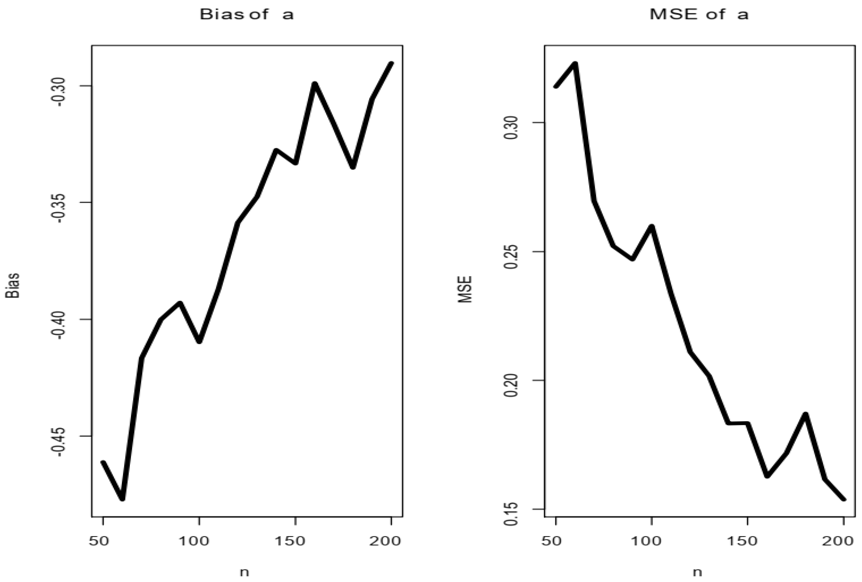
5. Simulation

In the discipline of statistics, simulation studies are becoming an increasingly common tool for evaluating the performance of a variety of estimating strategies. This is because simulation studies can replicate real-life conditions more accurately. In recent years, simulation studies have been increasingly popular due to the fact that they have the capacity to deliver a controlled and complete evaluation of various estimation approaches under a variety of different conditions. Because simulation studies can give this form of analysis, their growing popularity can be related to this capability. This paper makes an effort to highlight the statistical relevance of simulation studies as well as the driving reasons behind those studies’ research when it comes to evaluating estimation methodologies in this context by focusing on both the driving reasons behind those studies’ research and the statistical relevance of those studies. The mean squared error (MSE) is a performance indicator that is used extensively in simulation studies to assess the precision of a statistical model or estimator. Its name comes from the fact that it squares the error. It got its name from the fact that its value when squared is the same as its value when it was first calculated. It gets its name from the fact that the value of its squared representation is the same as that of its initial representation. This is the reason why its squared representation has the same value as its initial representation. It is an abbreviation that refers for “mean square error,” and its meaning is as follows: “the average of the squared discrepancies between the estimated values and the actual values of the parameter being estimated”. MSE is an acronym that stands for “mean square error.” The mean squared error, also known as MSE, is favored over measurements of dispersion and biases in simulation studies for a variety of reasons, some of which include the following: This is an in-depth study that takes into account everything that was mentioned before. The relative standard error (MSE) takes into account both the bias and the variability of the estimator. The measures of dispersion, such as variance and standard deviation, record only the variability of the estimator. The measures of bias, on the other hand, simply show the difference between the estimated and the actual values. Measures of error and bias are two different names for the same thing. Consideration is given to the algorithm that is outlined below:

(1)

Generate $N$ = 1000 samples of size $\mathcal{n}{|}_{\left(\mathcal{n}=50,55,\dots ,200\right)}$ from the GOGELx distribution;

(2)

Compute the MLEs for the $N=1000$ samples;

Compute the SEs of the MLEs for the 1000 samples;

(3)

The standard errors (STEs) can be computed by inverting the information matrix;

(4)

Obtain the MSE and for $h=a,b,\tau ,\sigma$ and $\mathcal{n}{|}_{\left(\mathcal{n}=50,60,\dots ,200\right)}$

The “R” program is used to perform the graphical simulations, where the following function is considered while drawing the plots; “seq(10,200,by = 10)” and the main code is:

• N = NN[i]
• cat(“i=”,i,“ n=”,N,‘\n’)
• ml = matrix(NA, nr=M, nc=4, byrow=T)
• j = 1
• while(j <= M){
• P = log(1-(runif(N))^(1/b))
• Q = ((-P)/(1-P))^(1/a)
• x = sigma*((1-(Q)^(-1/tau))-1)
• fit = goodness.fit(pdf=pdf_ GOGELx, cdf=cdf_ GOGELx, starts=c(1,1,1,1), data=x, method=“”, domain=c(0,Inf), mle=NULL)
• if(fit$Convergence == 0) {
• ml[j,] = fit$mle
• j = j + 1}

The plots of the biases against the n values, which range from 50 to 200, may be seen in the left panels of Figure 2, Figure 3, Figure 4 and Figure 5. The MSEs for $a,b,\tau ,\sigma$ are presented against n values of 50, 60, and 200, respectively, in Figure 2, Figure 3, Figure 4 and Figure 5. These values can be viewed in the right panels of those figures. It can be seen how the biases shift depending on the sample size n in the left panels of Figure 2, Figure 3, Figure 4 and Figure 5. Figure 5 shows this information graphically. In the panels on the right side of Figure 2, Figure 3, Figure 4 and Figure 5, we can observe how the four MSEs shift in response to an increase or decrease in the total number of samples. As n becomes smaller, the biases for $a,b,\tau ,\sigma$ tend to become negative and increasingly closer to zero, as can be seen in the left panels of Figure 2, Figure 3, Figure 4 and Figure 5. As n decreases, it is clear by looking at the right panels of Figure 2, Figure 3, Figure 4 and Figure 5 that the MSEs become closer and closer to zero as the number of observations decreases.

6. Applications

Datasets with heavy tails, in which extreme events occur more frequently than one would anticipate, are frequently modeled using the Lx distribution. In banking and insurance, this distribution is frequently used to simulate extreme occurrences like significant insurance claims or stock market crashes. It is crucial to pick a distribution that closely matches the data when modeling high-value datasets. To achieve this, the data should be compared to the distribution using statistical tests and visualizations. Once a suitable distribution is identified, it can be used to forecast upcoming extreme occurrences and determine the risk involved. In this Section, we analyze two real-life datasets with no extreme values. The two datasets are used in two applications to illustrate the importance, applicability, and flexibility of the GOGELx model in dealing with data that has no extreme values. The fits of the GOGELx are compared to some popular competing models as shown in

Table 2. Competitive models.

Special generalized mixture Lx (SGMLx)	Chesneau and Yousof [18]
Kumaraswamy-Lx (KumLx)	Lemonte and Cordeiro [19]
Beta-Lx (BLx)	Lemonte and Cordeiro [19]
Lx	Lomax [20]
Gamma-Lx (GamLx)	Cordeiro et al. [21]
Odd-loglogistic-Lx (OLLLx)	Altun et al. [22]
Transmute-Topp-Leone Lx (TTLLx)	Yousof et al. [23]
Reduced TTLLx (RTTLLx)	Yousof et al. [23]
Proportional reversed hazard rate Lx (PRHRLx)	New
Reduced GOGELx (RGOGELx)	New
Reduced-OLLLx (R-OLLLx)	Altun et al. [24]
Exponentiated-Lx (Exp-Lx)	Gupta et al. [25]
Reduced-Burr-Hatke-Lx (R-BHLx)	Yousof et al. [26]

.

Real data modeling under a new probability distribution is an important aspect of statistical analysis and machine learning. It allows us to understand and make predictions about real-life phenomena that may not follow traditional or well-known distributions.

I.

Real-life data often exhibit characteristics that cannot be accurately described using common probability distributions, such as normal, exponential, or Poisson distributions. By modeling data under a new probability distribution, we can capture the nuances and complexities of the data, leading to a more accurate representation of the underlying phenomenon.

II.

If we attempt to model real-life data using a distribution that does not accurately capture its characteristics, our predictions and inferences may be misleading or inaccurate. By utilizing a new probability distribution that closely matches the data, we can improve the accuracy of the predictions and make more reliable decisions based on the modeling results.

III.

Different domains may have unique characteristics and data patterns that are not adequately captured by standard probability distributions. For example, financial data often exhibit heavy-tailed or skewed distributions due to extreme events or outliers. By tailoring the modeling approach to the specific domain and using a new probability distribution, we can better understand the underlying processes and derive insights that are directly applicable to the domain of interest.

IV.

Real data modeling under a new probability distribution can reveal previously unseen patterns, relationships, or anomalies. By exploring alternative distributions, we may discover new statistical properties or uncover hidden dependencies that were not apparent using traditional approaches. This can lead to valuable insights, scientific discoveries, or improved decision making in various fields.

V.

Traditional statistical models and machine learning algorithms often assume specific distributions for simplicity and tractability. However, these assumptions may not hold in real-life scenarios, leading to biased or unreliable results. Modeling data under a new probability distribution can enhance the robustness and generalizability of the analysis, allowing the model to handle a wider range of data and perform well in different contexts.

VI.

Modeling real data under a new probability distribution provides a framework to quantify and characterize uncertainties. By accurately representing the data distribution, we can estimate confidence intervals, calculate prediction intervals, or perform Monte Carlo simulations to capture the inherent uncertainty in the modeling process. This information is crucial for decision making and risk assessment in various applications.

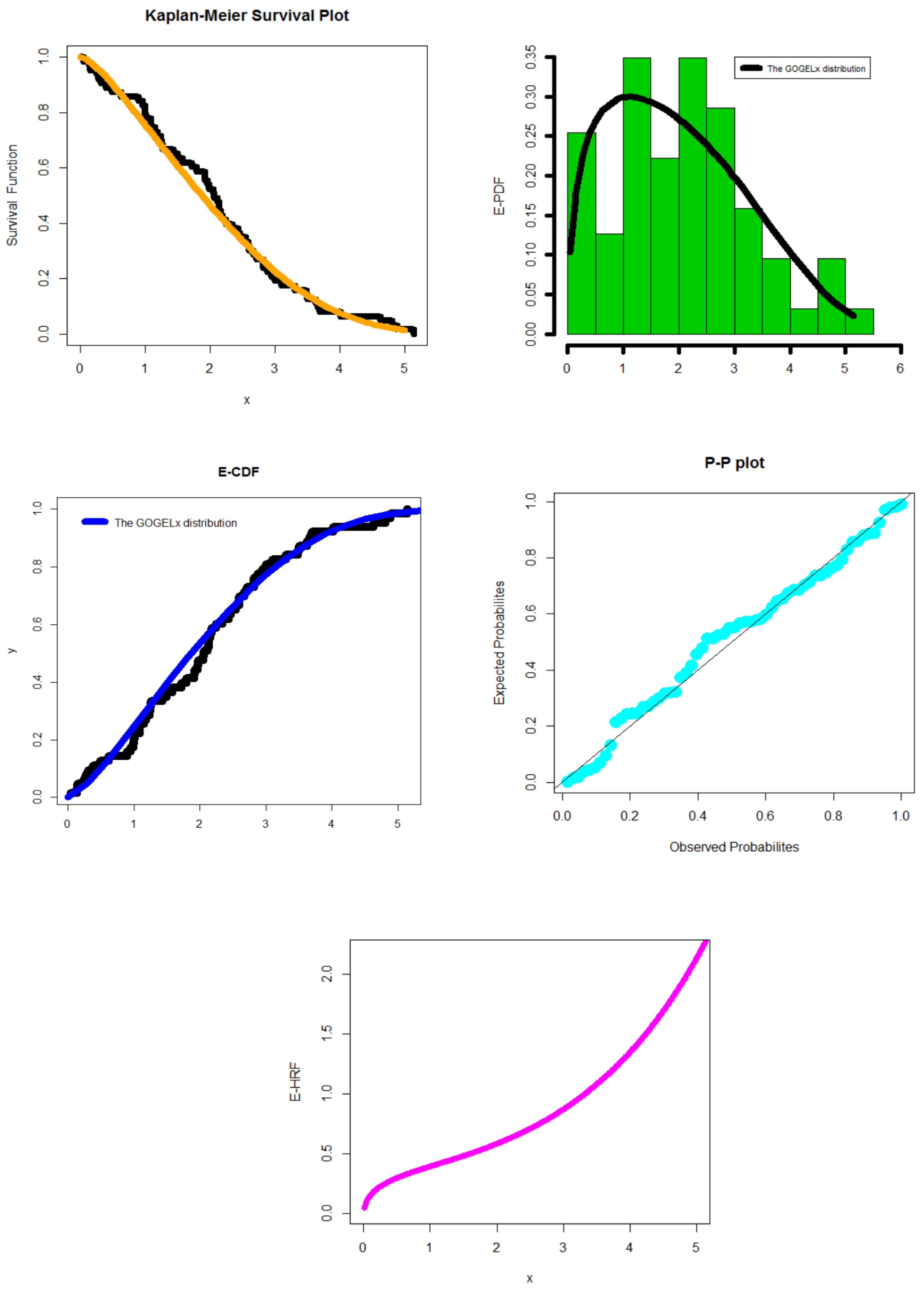
6.1. First Dataset

The statistics on the “failure times” of 84 aircraft windshields are presented in Murthy et al. [27]. This is the first true dataset, and it is represented by dataset I. The data are as follows: 1.866, 2.3850, 2.820, 0.0400, 3.00, 4.035, 1.281, 2.0850, 1.876, 2.4810, 3.467, 0.309, 1.8990, 2.610, 3.4780, 0.557, 1.9110, 2.625, 3.5780, 0.943, 1.9120, 2.632, 3.5950, 1.0700, 1.914, 1.2810, 2.038, 1.1240, 2.902, 4.167, 1.4320, 2.097, 2.934, 4.2400, 1.480, 2.135, 2.962, 1.981, 3.699, 3.443, 0.3010, 4.2550, 1.505, 2.154, 2.9640, 4.278, 1.506, 2.190, 3.000, 2.661, 2.890, 4.121, 2.6460, 4.3050, 1.568, 2.1940, 3.103, 4.376, 1.615, 2.2230, 3.114, 4.449, 1.6190, 2.224, 3.1170, 4.485, 1.652, 2.2290, 3.166, 4.570, 1.652, 2.3000, 3.344, 4.602, 1.7570, 3.7790, 1.248, 2.0100, 2.688, 3.9240, 1.3030, 2.089, 2.324, 3.3760, and 4.663. The presentation of the value of failure times for 84 aircraft windshields by Murthy et al. [27] can be used in a number of ways in the fields of aviation and reliability engineering. Understanding how long windshields last is important for figuring out how safe they are and how to handle any risks that come with running them. By looking at how long it takes for a windshield to break, researchers and engineers can find patterns or trends that could point to problems with the windshield’s design, materials, or care. This knowledge can be used to make safety procedures better and reduce the chances of problems occurring during a flight. The times when windshields break can give us an idea of how long and how well they are supposed to last. By looking at how windshields break, maintenance workers can come up with effective maintenance plans and replacement schedules to ensure that windshields are fixed or changed before they break dangerously. This preventative method can help prevent unexpected problems from occurring in the air, cut down on downtime, and reduce maintenance costs. Failure time data can be used to build reliability models that predict the likelihood of failure over time. Researchers can create models that describe how windshields break by fitting the data with correct statistical distributions. Then, these models can be used to predict dependability, improve the system design, and figure out what makes aircraft windshields less reliable. In short, the failure time data for aircraft windshields that Murthy et al. [27] provided are important for evaluating safety, planning maintenance, modeling reliability, controlling quality, thinking about insurance, and conducting research and development. By looking at this data, people in the aviation business can improve safety, streamline operations, and make aircraft windshields more reliable in general.

6.2. Second Dataset

The second authentic dataset, which is marked by the title “data set II,” includes information on the “service times” of sixty-three aircraft windshields. This information can be found in the study by Murthy et al. [27]. The data are as follows: 1.0030, 1.436, 0.1400, 0.2800, 1.7940, 2.819, 2.592, 0.3130, 0.0460, 1.9150, 2.820, 0.3890, 1.9200, 2.878, 3.1020, 0.9520, 2.0650, 3.3040, 0.9960, 2.1170, 3.483, 1.0030, 2.1370, 3.500, 0.487, 1.9630, 2.950, 0.6220, 1.978, 3.0030, 0.9000, 2.0530, 1.0100, 2.141, 3.6220, 1.492, 2.600, 0.150, 1.580, 2.163, 3.6650, 1.092, 2.183, 3.6950, 1.1520, 2.2400, 4.015, 2.670, 0.248, 1.7190, 2.717, 1.085, 1.183, 2.3410, 4.628, 1.2440, 2.435, 4.806, 1.249, 2.4640, 4.881, 1.262, 2.5430, and 5.140. The “service times” of 63 aircraft windshields, as reported by Murthy et al. [27], can provide valuable insights into the operational aspects and performances of these components. Service times data allows maintenance personnel to understand the average duration for which an aircraft windshield remains in service before it requires replacement or repair. By analyzing the service times, maintenance schedules can be optimized to ensure timely replacement or maintenance of windshields, minimize the risk of failures during operation, and improve overall aircraft reliability. Service times data can be used to analyze the reliability of aircraft windshields. Statistical techniques such as survival analysis can be applied to estimate the probability of a windshield surviving beyond a certain service time. This analysis aids in understanding the failure characteristics of windshields and can assist in reliability prediction and optimization efforts. By analyzing service times, manufacturers can assess the quality and performance of their windshields. Deviations from expected service times may indicate variations in the manufacturing process, material quality, or design flaws. This information can be used to improve quality control measures and identify areas for process improvement, resulting in higher-quality windshields with longer service lives.

Publications such as Mansour et al. [16], Elbiely and Yousof [7], Ibrahim and Yousof [6], Aryal et al. [28], Yousof et al. [29,30], Yadav et al. [8], and Goual et al. [31,32] are just a few examples of studies that include many other useful real-life datasets. A non-parametric technique called kernel density estimation (KDE) is used to calculate the probability density function of a random variable from a set of observations. The estimated density of the data is depicted graphically in the KDE plot. In a KDE plot, a kernel function—typically a bell-shaped curve centered at the location of the observation—represents each observation in the data collection. The estimated probability density function is produced by adding the kernel functions. The KDE plot’s smoothness depends on the kernel’s bandwidth. A smoother plot can be produced with a wider bandwidth than a more detailed plot with a lower bandwidth. Making the best bandwidth choice is a crucial stage in the estimation process because it has an impact on the KDE plot’s precision and clarity. When the underlying distribution is unknown or the dataset is too small to fit a parametric distribution, the KDE plot is frequently used in data analysis to visualize the distribution of a dataset. The distributions of two or more datasets can be compared using KDE plots, and the trends and abnormalities in the data can be found. KDE charts are sensitive to bandwidth and kernel selection, which is a key factor to keep in mind while reading them. The nonparametric KDE is used for investigating the initial form of the real data (see Figure 6). Nonparametric KDEs are shown in Figure 6.

The box plot in Figure 7, which was used to explore the extremes, shows that no extremes were discovered.

A graphical tool used to compare the distribution of a set of data to a theoretical distribution is called a quantile–quantile plot, or Q-Q plot in short. The quantiles of the dataset are compared to their corresponding quantiles of the theoretical distribution to produce the Q-Q plot. In other words, it compares the observed values to the predicted values. The points on the plot follow a straight line if the two sets of quantiles are comparable. A Q-Q plot is used to determine visually whether a dataset adheres to a specific distribution, such as a normal distribution. If the plot’s points are all in a straight line, the chosen distribution has performed well in simulating the dataset. The Q-Q plot is drawn to verify normality (see Figure 8). It can be seen in Figure 8 that normalcy was almost present.

The total time in test (TTT) plot (see Aarset [33]) is presented in Figure 9 to examine the HRF’s form. According to Figure 9, the HRF is “monotonically increasing” for the two sets of real-life data.

The Akaike information criterion (AKIC), the Bayesian information criterion (BYIC), the consistent Akaike information criterion (C-AKIC), the Hannan–Quinn information criterion (HNQIC), the Anderson and Darling (ADg), and the Cramér–von Mises (CVMs) are all used in the process of comparing various competing models. However, many other information tests can be used due to Aboraya et al. [34], Abdul-Moniem and Abdel-Hameed [35], Ali et al. [36], Ali et al. [37], Atkinson and Harrison [38], Ansari et al. [39], Cordeiro et al. [40], Durbey [41], Hamed et al. [42], Harris [43], Hassan and Al-Ghamdi [44], Gad et al. [45]. In addition to this, the applicable P-value and the Kolmogorov–Smirnova test are both taken into consideration. When it comes to a general fit of the data, it is generally accepted that the values of these statistics are a better fit when they are lower. The analytical results that were derived from the “Failure times” dataset are presented in

Table 3. The MLEs and (STEs) for “failure times” data for all the competing probability models.

Model	Estimates (STEs)
GOGELx(a,b,τ,σ)	2.25105	1.10598	6254.02	13,008.31
	(1.83474)	(0.74238)	(1836.7)	(573.462)
TTLLx(a,b,τ,σ)	−0.807522	2.47663	(15,608.2)	(386,228)
	(0.13961)	(0.54176)	(1602.37)	(123.943)
KumLx(a,b,τ,σ)	2.615042	100.2760	5.27716	78.6775
	(0.38226)	(120.488)	(9.8117)	(186.4111)
BLx(a,b,τ,σ)	3.603603	33.63872	4.83074	118.874
	(0.6187)	(63.7145)	(9.2382)	(428.993)
PRHRLx(b,β,ξ)	3.723 × 106	4.71 × 10−1	4.5 × 106
	1.312 × 106	(0.00011)	37.1470
RTTLLx(a,b,β)	−0.84732	5.520572	1.15678
	(0.10010)	(1.184791)	(0.09592)
SGMLx(a,β,ξ)	−1.04 × 10−1	9.831 × 106	1.18 × 107
	(0.12223)	(4843.33)	(501.043)
OLLLx(a,β,ξ)	2.326363	(7.17 × 105)	2.342 × 106)
	(2.14 × 10−1)	(1.19 × 104)	(2.613 × 101)
GamLx(a,β,ξ)	3.587602	52,001.49	37,029.66
	(0.51333)	(7955.00)	(81.16441)
Exp−Lx(a,β,ξ)	3.626101	20074.51	26257.68
	(0.623612)	(2041.831)	(99.74177)
R−OLLLx(a,β)	3.890564	0.5731643
	(0.36524)	(0.01946)
R−BHLx(β,ξ)	10,801,754	513,670,891
	(9,833,192)	(2,323,222)
Lx(β,ξ)	51,425.362	131,789.61
	(5932.492)	(296.0193)

and

Table 4. Results of the -ℓ and other statistics for “failure times” data for all the competing probability models.

Model	-ℓ	AKIC	C-AKIC	BYIC	HNQIC	ADg	CVMs	KS (p-Value)
GOGELx	129.6054	267.2108	267.7172	276.9341	271.1195	0.6334	0.0705	0.0716 (0.8716)
OLLLx	134.4235	274.8470	275.1470	282.1394	277.7785	0.9407	0.1009	0.0776 (0.7822)
TTLLx	135.5700	279.1400	279.6464	288.8633	283.0487	1.1257	0.1270	0.0799 (0.7201)
GamLx	138.4042	282.8083	283.1046	290.1363	285.7559	1.3666	0.1618	0.0802 (0.7199)
BLx	138.7177	285.4354	285.9354	295.2060	289.3654	1.4084	0.1680	0.0833 (0.7190)
Exp-Lx	141.3997	288.7994	289.0957	296.1273	291.7469	1.7435	0.2194	0.0866 (0.7187)
R-OLLLx	142.8452	289.6904	289.8385	294.5520	291.6447	1.9566	0.2554	0.0900 (0.7182)
SGMLx	143.0874	292.1747	292.4747	299.4672	295.1062	1.3467	0.1578	0.0924 (0.7180)
RTTLLx	153.9809	313.9618	314.2618	321.2542	316.8933	3.7527	0.5592	0.0939 (0.7170)
PRHRLx	162.8770	331.7540	332.0540	339.0464	334.6855	1.3672	0.1609	0.0950 (0.7151)
Lx	164.9884	333.9767	334.1230	338.8620	335.9417	1.3976	0.1665	0.0944 (0.7133)
R-BHLx	168.6040	341.2081	341.3562	346.0697	343.1624	1.6711	0.2069	0.0971 (0.7111)

, respectively. The MLEs and STEs for the dataset titled “Failure times” are shown in Table 3. In Table 4, the values for all goodness-of-fit tests for the dataset titled “Failure times” are shown. The results of the analyses conducted on the dataset titled “Service times” are presented in

Table 5. MLEs and STEs for “service times” data for all the competing probability models.

Model	Estimates (STEs)
GOGELx(a,b,τ,σ)	2.546132	0.593723	110.2577	224.6193
	(0.62763)	(0.09477)	(623.014)	(450.5222)
BLx(a,b,τ,σ)	1.921811	30.999493	4.968421	168.5724
	(0.31842)	(316.8218)	(50.5281)	(330.223)
TTLLx(a,b,τ,σ)	(−0.6277)	1.7858821	2122.393	4823.798
	(0.21371)	(0.415221)	(163.9125)	(200.219)
KumLx(a,b,τ,σ)	1.669151	60.56752	2.564912	64.06404
	(0.25722)	(86.0131)	(4.75897)	(176.599)
PRHRLx(a,β,ξ)	1.6666 × 106	3.899 × 10−1	1.338 × 106
	2.112 × 103	0.0014 × 10−1	0.985 × 106
RTTLLx(a,b,β)	−0.671425	2.744962	1.012384
	(0.187462)	(0.669612)	(0.114051)
SGMLx(a,β,ξ)	−1.04 × 10−1	6.4511 × 106	6.334 × 106
	(4.13 × 10−10)	(3.2142 × 106)	(3.854734)
OLLLx(a,β,ξ)	1.664193	6.348 × 105	2.015 × 106
	(1.79 × 10−1)	(1.73 × 104)	7.252 × 106
GamLx(a,β,ξ)	1.907323	35,842.433	39,197.557
	(0.321323)	(6945.073)	(151.6553)
Exp-Lx(a,β,ξ)	1.91453	22,971.153	32,881.999
	(0.34821)	(3209.553)	(162.2302)
R-OLLLx(a,β)	2.372331	0.691209
	(0.268253)	(0.044915)
R-BHLx(β,ξ)	14,055,512	53,203,423
	(422.0131)	(28.52323)
Lx(β,ξ)	99,269.83	207,019.41
	(11,863.52)	(301.2374)

and

Table 6. Results of the -ℓ and other statistics for “service times” data for all the competing probability models.

Model	-ℓ	AKIC	C-AKIC	BYIC	HNQIC	ADg	CVMs	KS (p-Value)
GOGELx	98.92234	205.8447	206.5343	214.4172	209.2163	0.4389	0.0721	0.0995 (0.75531)
KumLx	100.8676	209.7353	210.4249	218.3078	213.1069	0.7391	0.1219	0.1001 (0.73769)
TTLLx	102.4498	212.8996	213.5893	221.4722	216.2713	0.9431	0.1554	0.1002 (0.72560)
GamLx	102.8332	211.6663	212.0730	218.0958	214.1951	1.1120	0.1836	0.1002 (0.71561)
SGMLx	102.8940	211.7881	212.1949	218.2175	214.3168	1.1134	0.1839	0.1002 (0.71500)
BLx	102.9611	213.9223	214.6119	222.4948	217.2939	1.1336	0.1872	0.1002 (0.70206)
Exp-Lx	103.5498	213.0995	213.5063	219.5289	215.6282	1.2331	0.2037	0.1002 (0.70233)
OLLLx	104.9041	215.8082	216.2150	222.2376	218.3369	0.9424	0.1545	0.1003 (0.6978)
PRHRLx	109.2986	224.5973	225.004	231.0267	227.126	1.1264	0.1861	0.1005 (0.6944)
Lx	109.2988	222.5976	222.7976	226.8839	224.2834	1.1265	0.1861	0.1003 (0.6956)
R-OLLLx	110.7287	225.4573	225.6573	229.7436	227.1431	2.3472	0.3908	0.1004 (0.6001)
RTTLLx	112.1855	230.3710	230.7778	236.8004	232.8997	2.6875	0.4532	0.1006 (0.58801)

, respectively. Table 5 provides an overview of the MLEs and STEs that were collected for the “Service times” dataset. Table 6 contains the results of all of the goodness-of-fit tests conducted on the “Service times” dataset. As can be observed in Table 4 and Table 6, the GOGELx model has the lowest values for the AKIC, C-AKIC, BYIC, HNQIC, ADg, and CVMs of all the fitted models. This can be attributed to the fact that the GOGELx model was the most accurate. The fact that the GOGELx model was selected is evidence of this. It is feasible, in light of all of the factors considered, that this model will be selected as the model of choice.

For “failure times” and “service times,” Figure 10 and Figure 11, respectively, show the estimated Kaplan–Meier survival (E-KMSF) plot, estimated PDF (E-PDF), estimated CDF (E-CDF), probability–probability (P-P) plot, and estimated HRF (E-HRF).

7. Conclusions and Discussion

This study proposed and investigated the generalized new four-parameter lifespan model called the odd-generalized exponential Lomax (GOGELx) distribution. Asymmetric right-skewed, symmetric, asymmetric left-skewed, and uniform density are all possible for the GOGELx density function. The GOGELx model’s failure rate can be either monotonically decreasing, monotonically increasing, or constant. Most mathematical conclusions and derivations can be derived using the GOGELx density, which can be stated as a combination of the exponentiated Lx model. The GOGELx distribution can have either a positive (right skewness) or negative (left skewness) skewness. Its kurtosis spread ranges from 3.970398 to 38,056.81. We used the Farlie–Gumbel–Morgenstern copula, its modified counterpart, the Clayton copula, and Renyi’s copula in order to produce a few innovative bivariate versions of the GOGELx model. These copulas are called the Farlie–Gumbel–Morgenstern copula, the Clayton copula, and Renyi’s copula. The GOGELx model was utilized in order to produce these variations. This was performed with the intention of enhancing the mathematical component of the investigation that is now being carried out. In addition to that, the multivariate GOGELx model is demonstrated by employing the Clayton copula as a means of elucidation in this paper. On the other hand, it is probable that some of the studies that will be conducted in the future will be dedicated to the new multivariate and bivariate models. This is further discussed in the next paragraph. The technique of estimating the GOGELx parameters uses a strategy that maximizes the probability that an event will take place. This method is called the GOGELx likelihood method. In order to examine the finite sample behavior of the maximum likelihood estimators, we conducted a range of simulation experiments. These experiments were carried out using a simulation software. In this undertaking, the “biases” and the “mean squared errors” functioned as some of the most important instruments. It is essential to keep in mind that the biases for all parameters are virtually always negative and approach zero as the value of n approaches infinity. This is one of the most crucial aspects to keep in mind. On the other hand, when the value of n grows closer to infinity, the mean squared errors for all the parameters continue to become increasingly closer to zero.

The GOGELx distribution has a heavy tail, meaning that it assigns a non-negligible probability to extreme events. This property makes it useful for modeling rare events such as large losses or extreme values. The GOGELx distribution is used in reliability analysis to model the timing of a system or component failure, which can be a popular choice because it is flexible and can handle censored data. In future studies, the GOGELx distribution can be also used in finance to model extreme events, such as stock market crashes or large losses. It is often used in risk management to estimate the tail risk of a portfolio or an investment. The GOGELx distribution may also be used in insurance to model extreme events such as natural disasters, which can result in large losses. It is used to estimate the probability of the occurrence of these events and to price insurance policies accordingly.

In potential future studies, some applications of big data in transportation under the probability distribution theory may be addressed. The application of big data in transportation, coupled with the probability distribution theory, enables advanced analysis, prediction, and optimization. By leveraging the vast amounts of available data, transportation planners can make data-driven decisions, improve system efficiency, enhance safety, and provide better services to travelers. (See Schumann et al. [4]). According to Schumann et al. [4], the meteoric rise in the popularity of micro-mobility presents considerable issues in terms of building its systems, assuring its safety, addressing its social repercussions, and minimizing its negative effects on the environment. In the meantime, micro-mobility is distinguished by its abundance of big data that are passively generated and possess significant potential to help solve problems. Although there has been an increase in recent studies that use data on micro-mobility generated passively, knowledge and discoveries are scattered, which limits the value of the obtained data. This paper includes a contemporary analysis of how micro-mobility research and practice have used passively generated big data and their applications to address the major difficulties associated with micro-mobility. The purpose of this paper is to fill this gap that has been identified. Even though it has obvious benefits in terms of coverage, resolution, and the elimination of human errors, passively generated big data need to be handled with attention to bias, inaccuracy, and privacy concerns before they can be used effectively. This paper also brings to light issues that require additional investigation and offers fresh perspectives on how micro-mobility may be made safer, more efficient, more ecological, and more equal. The integration of big data and the probability distribution theory in transportation has the potential to transform industries and create a more sustainable and intelligent transportation ecosystem. Big data have transformed various industries, including transportation, by providing valuable insights and enabling informed decision making. When applying big data in transportation, probability distribution theory plays a crucial role in analyzing and predicting various outcomes. Let us delve into the discussion on how big data and probability distribution theory intersect in the transportation domain.

I.

Big data sources, such as traffic sensors, GPS data, and social media feeds, generate vast amounts of information regarding traffic patterns. By analyzing this data using probability distribution theory, transportation planners can model and predict traffic flow. Probability distributions, such as Poisson or Gaussian distributions, can be used to describe the frequency and duration of traffic congestion, accidents, or other events. This analysis helps in optimizing traffic management strategies, such as signal timing, route planning, and congestion mitigation.

II.

Transportation systems need to anticipate future demands to optimize operations and allocate resources efficiently. The probability distribution theory can be employed to model demand patterns based on historical data. By analyzing big data on factors like population density, demographics, weather, and events, transportation planners can develop probabilistic models to forecast travel demands. These models can help in determining the need for additional infrastructure, adjusting transit schedules, and optimizing fleet deployment.

III.

The probability distribution theory is useful for predicting equipment failures and optimizing maintenance schedules. By analyzing big data collected from sensors embedded in vehicles, trains, or infrastructure, probabilistic models can be built to predict the likelihood and timing of component failures. This enables proactive maintenance, reduces unplanned downtime, and improves the overall system reliability. Probability distributions, such as the Weibull distribution, can help in estimating the remaining useful life of assets and optimizing maintenance resources.

IV.

Big data analytics combined with probability distribution theory can enhance safety in transportation. By analyzing historical accident data, weather conditions, road characteristics, and other relevant factors, transportation agencies can model accident probabilities and severity. These models can identify high-risk areas and support the development of targeted safety interventions. By understanding the probability distributions of different types of accidents, transportation planners can allocate resources effectively to reduce fatalities and injuries.

V.

Intelligent transportation systems leverage big data and the probability distribution theory to improve traffic efficiency and safety. By integrating data from various sources, such as traffic cameras, vehicle sensors, and weather stations, probabilistic models can be developed to optimize signal timing, manage adaptive traffic control systems, and enable real-time incident detection. These models can help predict travel times, estimate congestion levels, support dynamic route guidance, and enhance the overall system performance.

References

- Tadikamalla, P.R. A look at the Burr and realted distributions. Int. Stat. Rev. 1980, 48, 337–344. [Google Scholar] [CrossRef] [Green Version]
- Corbellini, A.; Crosato, L.; Ganugi, P.; Mazzoli, M. Fitting Pareto II distributions on firm size: Statistical methodology and economic puzzles. In Proceedings of the International Conference on Applied Stochastic Models and Data Analysis, Chania, Greece, 29 May–1 June 2007. [Google Scholar]
- Alizadeh, M.; Ghosh, I.; Yousof, H.M.; Rasekhi, M.; Hamedani, G.G. The generalized odd-generalized exponential family of distributions: Properties, characterizations and applications. J. Data Sci. 2017, 15, 443–466. [Google Scholar] [CrossRef]
- Schumann, H.H.; Haitao, H.; Quddus, M. Passively generated big data for micro-mobility: State-of-the-art and future research directions. Transp. Res. Part D Transp. Environ. 2023, 121, 103795. [Google Scholar] [CrossRef]
- Afify, A.Z.; Nofal, Z.M.; Yousof, H.M.; El Gebaly, Y.M.; Butt, N.S. The transmuted Weibull Lomax distribution: Properties and application. Pak. J. Stat. Oper. Res. 2015, 11, 135–152. [Google Scholar] [CrossRef] [Green Version]
- Ibrahim, M.; Yousof, H.M. A new generalized Lomax model: Statistical properties and applications. J. Data Sci. 2020, 18, 190–217. [Google Scholar] [CrossRef]
- Elbiely, M.M.; Yousof, H.M. A new extension of the Lomax distribution and its Applications. J. Stat. Appl. 2018, 2, 18–34. [Google Scholar]
- Yadav, A.S.; Goual, H.; Alotaibi, R.M.; Rezk, H.; Ali, M.M.; Yousof, H.M. Validation of the Topp-Leone-Lomax model via a modified Nikulin-Rao-Robson goodness-of-fit test with different methods of estimation. Symmetry 2020, 12, 57. [Google Scholar] [CrossRef] [Green Version]
- Elsayed, H.A.; Yousof, H.M. A new Lomax distribution for modeling survival times and taxes revenue data sets. J. Stat. Appl. 2019, 2, 35–58. [Google Scholar]
- Farlie, D.J.G. The performance of some correlation coefficients for a general bivariate distribution. Biometrika 1960, 47, 307–323. [Google Scholar] [CrossRef]
- Morgenstern, D. Einfache beispiele zweidimensionaler verteilungen. Mitteilingsblatt Math. Stat. 1956, 8, 234–235. [Google Scholar]
- Gumbel, E.J. Bivariate logistic distributions. J. Am. Stat. Assoc. 1961, 56, 335–349. [Google Scholar] [CrossRef]
- Gumbel, E.J. Bivariate exponential distributions. J. Amer. Statist. Assoc. 1960, 55, 698–707. [Google Scholar] [CrossRef]
- Elgohari, H.; Yousof, H.M. A Generalization of Lomax Distribution with Properties, Copula and Real Data Applications. Pak. J. Stat. Oper. Res. 2020, 16, 697–711. [Google Scholar] [CrossRef]
- Ghosh, I.; Ray, S. Some alternative bivariate Kumaraswamy type distributions via copula with application in risk management. J. Stat. Theory Pract. 2016, 10, 693–706. [Google Scholar] [CrossRef]
- Mansour, M.; Yousof, H.M.; Shehata, W.A.M.; Ibrahim, M. A new two parameter Burr XII distribution: Properties, copula, different estimation methods and modeling acute bone cancer data. J. Nonlinear Sci. Appl. 2020, 13, 223–238. [Google Scholar] [CrossRef] [Green Version]
- Pougaza, D.B.; Djafari, M.A. Maximum entropies copulas. In Proceedings of the 30th International Workshop on Bayesian Inference and Maximum Entropy Methods in Science and Engineering 2011, Chamonix, France, 4–9 July 2010; pp. 329–336. [Google Scholar]
- Chesneau, C.; Yousof, H.M. On a special generalized mixture class of probabilistic models. J. Nonlinear Model. Anal. 2021, 3, 71–92. [Google Scholar]
- Lemonte, A.J.; Cordeiro, G.M. An extended Lomax distribution. Statistics 2013, 47, 800–816. [Google Scholar] [CrossRef]
- Lomax, K.S. Business failures: Another example of the analysis of failure data. J. Am. Stat. Assoc. 1954, 49, 847–852. [Google Scholar] [CrossRef]
- Cordeiro, G.M.; Ortega, E.M.; Popović, B.V. The gamma-Lomax distribution. J. Stat. Comput. Simul. 2015, 85, 305–319. [Google Scholar] [CrossRef]
- Altun, E.; Yousof, H.M.; Hamedani, G.G. A new log-location regression model with influence diagnostics and residual analysis. Facta Univ. Ser. Math. Inform. 2018, 33, 417–449. [Google Scholar] [CrossRef]
- Yousof, H.M.; Alizadeh, M.; Jahanshahiand, S.M.A.; Ramires, T.G.; Ghosh, I.; Hamedani, G.G. The Transmute-Topp-Leone G family of distributions: Theory, characterizations and applications. J. Data Sci. 2017, 15, 723–740. [Google Scholar] [CrossRef]
- Altun, E.; Yousof, H.M.; Chakraborty, S.; Handique, L. Zografos-Balakrishnan Burr XII distribution: Regression modeling and applications. Int. J. Math. Stat. 2018, 19, 46–70. [Google Scholar]
- Gupta, R.C.; Gupta, P.L.; Gupta, R.D. Modeling failure time data by Lehman alternatives. Commun. Stat.-Theory Methods 1998, 27, 887–904. [Google Scholar] [CrossRef]
- Yousof, H.M.; Altun, E.; Ramires, T.G.; Alizadeh, M.; Rasekhi, M. A new family of distributions with properties, regression models and applications. J. Stat. Manag. Syst. 2018, 21, 163–188. [Google Scholar] [CrossRef]
- Murthy, D.N.P.; Xie, M.; Jiang, R. Weibull Models; Wiley: Hoboken, NJ, USA, 2004. [Google Scholar]
- Aryal, G.R.; Ortega, E.M.; Hamedani, G.G.; Yousof, H.M. The Topp Leone Generated Weibull distribution: Regression model, characterizations and applications. Int. J. Stat. Probab. 2017, 6, 126–141. [Google Scholar] [CrossRef]
- Yousof, H.M.; Ahsanullah, M.; Khalil, M.G. A New Zero-Truncated Version of the Poisson Burr XII Distribution: Characterizations and Properties. J. Stat. Theory Appl. 2019, 18, 1–11. [Google Scholar] [CrossRef]
- Yousof, H.M.; Majumder, M.; Jahanshahi, S.M.A.; Ali, M.M.; Hamedani, G.G. A new Weibull class of distributions: Theory, characterizations and applications. J. Stat. Res. Iran 2018, 15, 45–83. [Google Scholar] [CrossRef] [Green Version]
- Goual, H.; Yousof, H.M.; Ali, M.M. Lomax inverse Weibull model: Properties, applications, and a modified Chi-squared goodness-of-fit test for validation. J. Nonlinear Sci. Appl. (JNSA) 2020, 13, 330–353. [Google Scholar] [CrossRef] [Green Version]
- Goual, H.; Yousof, H.M. Validation of Burr XII inverse Rayleigh model via a modified chi-squared goodness-of-fit test. J. Appl. Stat. 2019, 47, 393–423. [Google Scholar] [CrossRef]
- Aarset, M.V. How to identify a bathtub hazard rate. IEEE Trans. Reliab. 1987, 36, 106–108. [Google Scholar] [CrossRef]
- Aboraya, M.; Ali, M.M.; Yousof, H.M.; Ibrahim, M. A Novel Lomax Extension with Statistical Properties, Copulas, Different Estimation Methods and Applications. Bull. Malays. Math. Sci. Soc. 2022, 45, 85–120. [Google Scholar] [CrossRef]
- Abdul-Moniem, I.B.; Abdel-Hameed, H.F. On exponentiated Lomax distribution. Int. J. Math. Arch. 2012, 3, 2144–2150. [Google Scholar]
- Ali, M.M.; Korkmaz, M.Ç.; Yousof, H.M.; Butt, N.S. Odd Lindley-Lomax Model: Statistical Properties and Applications. Pak. J. Stat. Oper. Res. 2019, 419–430. [Google Scholar] [CrossRef]
- Ali, M.M.; Yousof, H.M.; Ibrahim, M. A New Lomax Type Distribution: Properties, Copulas, Applications, Bayesian and Non-Bayesian Estimation Methods. Int. J. Stat. Sci. 2021, 21, 61–104. [Google Scholar]
- Atkinson, A.B.; Harrison, A.J. Distribution of Personal Wealth in Britain; Cambridge University Press: Cambridge, UK, 1978. [Google Scholar]
- Ansari, S.; Rezk, H.; Yousof, H. A New Compound Version of the Generalized Lomax Distribution for Modeling Failure and Service Times. Pak. J. Stat. Oper. Res. 2020, 16, 95–107. [Google Scholar] [CrossRef]
- Cordeiro, G.M.; Yousof, H.M.; Ramires, T.G.; Ortega, E.M.M. The Burr XII system of densities: Properties, regression model and applications. J. Stat. Comput. Simul. 2018, 88, 432–456. [Google Scholar] [CrossRef]
- Durbey, S.D. Compound gamma, beta and F distributions. Metrika 1970, 16, 27–31. [Google Scholar]
- Hamed, M.S.; Cordeiro, G.M.; Yousof, H.M. A New Compound Lomax Model: Properties, Copulas, Modeling and Risk Analysis Utilizing the Negatively Skewed Insurance Claims Data. Pak. J. Stat. Oper. Res. 2022, 18, 601–631. [Google Scholar] [CrossRef]
- Harris, C.M. The Pareto distribution as a queue service descipline. Oper. Res. 1968, 16, 307–313. [Google Scholar] [CrossRef]
- Hassan, A.S.; Al-Ghamdi, A.S. Optimum step stress accelerated life testing for Lomax distibution. J. Appl. Sci. Res. 2009, 5, 2153–2164. [Google Scholar]
- Gad, A.M.; Hamedani, G.G.; Salehabadi, S.M.; Yousof, H.M. The Burr XII-Burr XII distribution: Mathematical properties and characterizations. Pak. J. Stat. 2019, 35, 229–248. [Google Scholar]