Interval Forecasting Method of Aggregate Output for Multiple Wind Farms Using LSTM Networks and Time-Varying Regular Vine Copulas

Abstract

Interval forecasting has become a research hotspot in recent years because it provides richer uncertainty information on wind power output than spot forecasting. However, compared with studies on single wind farms, fewer studies exist for multiple wind farms. To determine the aggregate output of multiple wind farms, this paper proposes an interval forecasting method based on long short-term memory (LSTM) networks and copula theory. The method uses LSTM networks for spot forecasting firstly and then uses the forecasting error data generated by LSTM networks to model the conditional joint probability distribution of the forecasting errors for multiple wind farms through the time-varying regular vine copula (TVRVC) model, so as to obtain the probability interval of aggregate output for multiple wind farms under different confidence levels. The proposed method is applied to three adjacent wind farms in Northwest China and the results show that the forecasting intervals generated by the proposed method have high reliability with narrow widths. Moreover, comparing the proposed method with other four methods, the results show that the proposed method has better forecasting performance due to the consideration of the time-varying correlations among multiple wind farms and the use of a spot forecasting model with smaller errors.

1. Introduction

Owing to the intermittent and stochastic nature, the increasing penetration of wind power poses a big challenge to the power grid operation. Interval forecasting is a type of probabilistic forecasting that can provide the upper and lower boundaries of output wind power under a given confidence level [1]. Compared with a spot forecast, an interval forecast can provide more uncertain information for solving problems in power grid operation, such as unit commitment optimization, reserve plan making and operational risk assessment, and thus has been widely studied in recent years [2].

The methods of interval forecasting can be divided into three categories, namely, methods based on fitting probability distribution function (PDF) of spot forecasting errors, quantile regression methods and bound evaluation methods. Among them, a quantile regression method [3,4,5,6] obtains the forecasting intervals by constructing a regression model for multiple quantiles, and the complexity of the quantile regression model increases with the number of quantiles required and is computationally intensive. A bound evaluation method transforms the interval forecasting into an objective optimization problem [7,8], which can directly output the upper and lower edge values of wind power, this method usually requires machine learning algorithms because of the discontinuous optimization objectives. At the same time, the above two methods need to be remodeled when the required confidence level changes. A method based on fitting PDF of spot forecasting errors performs spot forecasting firstly and then calculates forecasting intervals by fitting the PDF of the spot forecasting error [1]. Although this method has more steps than the previous two methods, the wind power output intervals at all confidence levels can be obtained after the PDF of forecast errors is modeled. In addition, since most power dispatching departments already have the capability of short-term wind power spot forecasting, this method is the easiest to implement and be understood by dispatchers and is the most widely used.

For the methods based on fitting PDF of spot forecasting errors, both the spot forecast model and the PDF model will affect the forecasting results. Spot forecast models can be mainly categorized into physical models and the statistical learning models. A physical model uses numerical weather forecast data and geographic information to predict wind power [9]. The statistical learning model makes predictions by learning from historical data and finding the relationship between relevant data and wind power output; examples of this model include the time series model in ref. [10] and the Markov and autoregressive moving average (ARMA) models in ref. [11]. In recent years, with the continuous development of artificial intelligence theory, various artificial intelligence algorithms have also been incorporated into statistical learning methods [12,13,14,15,16]. Specifically, ref. [17,18] constructed a backpropagation (BP) neural network and ref. [19] constructed a support vector machine (SVM) model for wind power forecasting. The authors of ref. [1,20,21] used long short-term memory (LSTM) networks for spot forecasting, and ref. [22] established a spot forecasting model based on a deep Boltzmann machine. The use of artificial intelligence algorithms for the spot forecasting of wind power output has been a development trend. For the PDF modeling of spot forecasting error, a Gaussian distribution is used in ref. [23,24], and a beta distribution is used in ref. [25] to model the PDF of wind farm forecast error. The work in ref. [26] established a conditional PDF for the prediction errors through the copula function. In ref. [1], the nonparametric kernel density estimation was used to fit the PDF of the wind power prediction errors.

However, all the aforementioned studies involved an interval forecasting method for a single wind farm. With the introduction of the goals of carbon peaking and carbon neutrality, the proportion of wind power as clean energy in the power grid will be further expanded [27,28,29,30], so compared with a single wind farm, the power grid will be more concerned about the aggregate output of multiple wind farms. Interval forecasting methods for multiple wind farms include the extrapolation method [31], the upscaling method [32], the superposition method [33] and the high-dimensional copula method [34]. The extrapolation method predicts aggregate wind power by finding wind speed predictions that are similar to the current ones in the historical dataset; thus, the accuracy of prediction is strongly influenced by the accuracy of the weather forecasts. In the upscaling method, reference wind farms are selected, and the weighted sum of the forecast outputs of these reference wind farms is used as the aggregate output, but there is no standard for how to select the reference wind farms and weights. Superposition method adds the forecasting values of multiple single wind farms as the forecasting values of their aggregate output. However, this method ignores correlations among multiple wind farms due to their similar geographic locations and climatic conditions [35,36], and may have poor forecasting accuracy.

The high-dimensional copula model performs better than other models in terms of fitting the correlations of multidimensional variables and has been introduced into interval forecasting for multiple wind farms to model the PDF of forecasting errors in recent years. In ref. [34], the regular vine copula model was introduced to describe the joint PDF of the spot forecasts and real outputs of multiple wind farms. Then, the aggregate output for multiple wind farms can be derived from the joint PDF, and only one type of copula function is used in this correlation model. The work in ref. [37] constructs a regular vine copula model for multiple wind farms with more types of copula functions. The studies in ref. [35,37] both use static copula functions, but in practice, the correlations between multiple wind farms vary with time. The authors of ref. [38] used time-varying copulas to construct a drawable vine copula model, which considers time-varying correlations of multiple variables of wind farms, but only one type of copula function is used in the model, which may not be applicable to describe the correlation between multiple wind farms.

In summary, most of the existing interval forecasting studies focus on single wind farms, there are few studies on aggregate output of multiple wind farms. Additionally, the accuracy of the copula model used in interval forecasting of aggregate output for multiple wind farms needs to be improved. Moreover, the studies mentioned above rarely provide complete modeling processes stating how the copula model is combined with the spot forecasting model to achieve interval forecasting. To address these problems, the main contributions of this paper are as follows:

(1)

A time-varying regular vine copula model is proposed to obtain the conditional joint PDF of the forecasting errors of multiple wind farms. The proposed method not only uses multiple types of copula functions and optimize the structure of vine copula based on the Akaike information criterion (AIC), but also uses copula functions with time-varying dependence parameters to improve the model’s ability to capture the complex and time-varying correlations among multiple wind farms;

(2)

Interval forecasting is achieved for the aggregate output for multiple wind farms by combining the spot forecasting model based on LSTM networks and the time-varying regular vine copula model. In this method, the historical outputs of multiple wind farms are used to train the spot forecasting model based on LSTM networks. Then, using the forecasting outputs and errors generated by the trained spot forecasting model as modeling data, a time-varying regular vine copula model is established to obtain the conditional joint PDF of the forecasting errors; then, the confidence interval can be derived from this model. Finally, the confidence intervals of the aggregate output are obtained by adding up the confidence intervals of forecasting errors and the spot forecasting outputs. This modeling framework can also be applied to combine the copula model with other spot forecasting methods.

This paper is organized as follows. Section 2 proposes a time-varying regular vine copula model to obtain the conditional joint PDF of the forecasting errors. Section 3 proposes an aggregate output interval forecasting method based on LSTM networks and time-varying regular vine copulas (LSTM-TVRVC). Section 4 provides a case analysis and shows the experimental results and discussions, and Section 5 concludes the paper.

2. Conditional Joint PDF for the Forecasting Errors of Multiple Wind Farms Using Time-Varying Regular Vine Copulas

2.1. Sklar’s Theorem

A copula function is defined as the connection function between the joint distribution function of multiple variables and their marginal distribution functions [39]. For an s-dimensional variable $\left(g_1, g_2,\cdots , g_i,\cdots , g_s\right)$, according to Sklar’s theorem, there must be a copula function that satisfies (1).

$$F\left(g_1,g_2,\cdots ,g_i,\cdots ,g_s\right)=C\left(u_1,u_2,\cdots ,u_i,\cdots ,u_s\right)$$

(1)

where $u_i=F\left(g_i\right)$ is the cumulative probability distribution (CDF) of variable $g_i$, $F\left(·\right)$ is the CDF and $C\left(·\right)$ is the copula CDF.

The derivative of (1) is the corresponding s-dimensional joint PDF:

$$f\left(g_1,g_2,\cdots ,g_s\right)=c\left(u_1,u_2,\cdots u_s\right){\displaystyle \prod _{i=1}^{s}f\left(g_i\right)}$$

(2)

where $c\left(·\right)$ is the copula PDF and $f\left(g_i\right)$ is the marginal PDF of variable $g_i$.

Therefore, the joint PDF of multiple variables can be converted into a copula function and marginal distribution functions for multiple variables.

2.2. Regular Vine Copulas

As (1) shows, the copula function for multiple variables is equivalent to using only one type of copula function to establish the dependence structure between multidimensional variables; consequently, this function has great limitations. In addition, as the dimensionality of the variables increases, the scale of the parameters to be estimated for the high-dimensional copula function becomes larger, thus creating difficulties for equation solving.

The regular vine copula model transforms a high-dimensional copula function into a cascade of bivariate copula models [40], thus allowing for more types of copula functions to be used and making the correlation modeling process for multiple variables more flexible.

The regular vine copula model for s variables consists of $s-1$ trees denoted as $T_1,\cdots ,T_j,\cdots T_{s-1}$. The $j-\mathrm{th}$ tree contains $s-j$ nodes connected by $s-j-1$ edges. Each node corresponds to a CDF, and each edge corresponds to a bivariate copula model calculated from two nodes connected to the edge.

The node set and edge set of $T_j$ are denoted as $N_j$ and $E_j$, respectively, and regular vine copulas should satisfy the following conditions [37]:

① $T_1$ has s nodes, with a node set $N_1=\left\{1,2,\cdots ,s\right\}$ and an edge set $E_1$. ② Concerning $T_j$ $\left(2\le j\le s-1\right)$, $N_j$ equals $E_{j-1}$. ③ If two edges in $T_j$ are joined in $T_{j+1}$, the edges need to share a common node in $T_j$.

An edge in $E_j$ is denoted as $e=a\left(e\right),b\left(e\right)\left|D\left(e\right)\right.$, where $a\left(e\right)\left|D\left(e\right)\right.$ and $b\left(e\right)\left|D\left(e\right)\right.$ are two nodes connected by $e$ and $D\left(e\right)$ is the conditioning set. The copula PDF corresponding to this edge is denoted as $c_{a\left(e\right),b\left(e\right)|D\left(e\right)}\left(u_{a\left(e\right)|D\left(e\right)},u_{b\left(e\right)|D\left(e\right)}\right)$, where $u_{a\left(e\right)|D\left(e\right)}$ and $u_{b\left(e\right)|D\left(e\right)}$ denote CDFs corresponding to the two nodes connected by e; then, (2) can be transformed into:

$$f\left(g_1,g_2\cdots ,g_s\right)={\displaystyle \prod _{j=1}^{s-1}{\displaystyle \prod _{e\in E_j}{c}_{a\left(e\right),b\left(e\right)|D\left(e\right)}\left(u_{a\left(e\right)|D\left(e\right)},u_{b\left(e\right)|D\left(e\right)}\right)}}{\displaystyle \prod _{i=1}^{s}f\left(g_i\right)}$$

(3)

where $u_{a\left(e\right)|D\left(e\right)}=F\left(g_{a\left(e\right)}|g_{D\left(e\right)}\right)$ and $g_{D\left(e\right)}$ denotes the variables corresponding to $D\left(e\right)$ (the $D\left(e\right)$ of the tree $T_1$ is empty).

Figure 1 shows a possible structure of a six-dimensional regular vine copula model, where blocks denote nodes and lines denote edges.

As (3) and Figure 1 show, the regular vine copula model not only has more options in terms of the type of bivariate copula corresponding to each edge but can also freely adjust structures of trees as needed.

2.3. Time-Varying Copula Functions

When constructing the regular vine copula model, the type of bivariate copula corresponding to each edge needs to be determined. Copula functions can be divided into elliptical copulas and Archimedean copulas [41]. Elliptical copulas, which include Gaussian and t copulas, have symmetric tail correlations. Archimedean copulas, which include Gumbel and Clayton copulas, have asymmetric tails correlations. The dependence parameters of traditional copula functions are static; that is, these parameters do not change over time. However, the nonlinear correlations among the outputs of multiple wind farms often exhibit time-varying characteristics. Therefore, when constructing regular vine copulas, this paper uses the time-varying copula functions proposed by Patton as alternative copula functions, whose dependence parameters are akin to a restricted ARMA process [42,43].

The time-varying copula functions used in this paper and their evolution equation of the dependence parameters are as follows.

(3)

Time-varying Gaussian copula.

This copula has a symmetric distribution but does not reflect tail correlations. The functional form of this copula is shown in (4).

$$C_N\left(u_1,u_2;{\rho }_{N,t}\right)={\displaystyle \underset{-\infty }{\overset{{\Phi }^{-1}\left(u_1\right)}{\int }}{\displaystyle \underset{-\infty }{\overset{{\Phi }^{-1}\left(u_2\right)}{\int }}\frac{1}{2\pi \sqrt{1-{\rho }_{N,t}^2}}\exp \left(\frac{-\left(r^2+q^2-2{\rho }_{N,t}rq\right)}{2\left(1-{\rho }_{N,t}{}^2\right)}\right)}}drdq$$

(4)

where $u_1$ and $u_2$ are the marginal CDFs of two variables, ${\Phi }^{-1}\left(·\right)$ is the inverse of the standard Gaussian CDF and ${\rho }_{N.t}$ is the dependence parameter. The evolution equation of this copula is as follows:

$${\rho }_{N,t}=\Lambda \left({\omega }_N+{\beta }_N{\rho }_{t-1}+{\alpha }_N\frac{1}{10}{\displaystyle \sum _{j=1}^{10}{\Phi }^{-1}\left(u_{1,t-j}\right){\Phi }^{-1}\left(u_{2,t-j}\right)}\right)$$

(5)

where $\Lambda \left(x\right)=\left(1-e^{-x}\right)/\left(1+e^{-x}\right)$ is designed to keep ${\rho }_{N,t}\in \left(-1,1\right)$, and $u_{1,t-j}$ and $u_{2,t-j}$ are the CDFs of the two variables at moment $t-j$; the parameters to be estimated are $\left\{{\omega }_N,{\beta }_N,{\alpha }_N\right\}$.

(4)

Time-varying t copula.

$$C_T\left(u_1,u_2;{\rho }_{T,t},d_{T,t}\right)={{\displaystyle \underset{-\infty }{\overset{T^{-1}\left(u_1\right)}{\int }}{\displaystyle \underset{-\infty }{\overset{T^{-1}\left(u_2\right)}{\int }}\frac{1}{2\pi \sqrt{1-{\rho }_{T,t}^2}}\left(1+\frac{r^2+q^2-2{\rho }_{T,t}rq}{d_{T,t}\left(1-{\rho }_{T,t}{}^2\right)}\right)}}}^{-\frac{d_{T,t}+2}{2}}drdq$$

(6)

where $T^{-1}\left(·\right)$ is the inverse of the t CDF, ${\rho }_{T,t}$ and $d_{T,t}$ are the dependence parameters and the evolution equations of these parameters are as follows:

$$\begin{array}{l}{\rho }_{T,t}=\Lambda \left({\omega }_{{\rho }_T}+{\beta }_{{\rho }_T}{\rho }_{T,t-1}+{\alpha }_{{\rho }_T}\frac{1}{10}{\displaystyle \sum _{j=1}^{10}{T}^{-1}\left(u_{1,t-j}\right)T^{-1}\left(u_{2,t-j}\right)}\right)\\ d_{T,t}=\Lambda \left({\omega }_{d_T}+{\beta }_{d_T}{d}_{T,t-1}+{\alpha }_{d_T}\frac{1}{10}{\displaystyle \sum _{j=1}^{10}{T}^{-1}\left(u_{1,t-j}\right)T^{-1}\left(u_{2,t-j}\right)}\right)\end{array}$$

(7)

and the parameters to be estimated are $\left\{{\omega }_{{\rho }_T},{\beta }_{{\rho }_T},{\alpha }_{{\rho }_T}\right\}$, $\left\{{\omega }_{d_T},{\beta }_{d_T},{\alpha }_{d_T}\right\}$.

(5)

Time-varying Clayton copula.

This copula is suitable for variables with a strong lower tail correlation. The functional form is shown as (8).

$$C_C\left(u_1,u_2;{\theta }_{c,t}\right)=\max \left({\left(u_1^{-{\theta }_{C,t}}+u_2^{-{\theta }_{C,t}}-1\right)}^{-\frac{1}{{\theta }_{C,t}}},0\right)$$

(8)

where ${\theta }_{C,t}$ is the dependence parameter and its evolution equation is as follows:

$${\theta }_{C,t}=\Lambda \left({\omega }_C+{\beta }_C{\theta }_{C,t-1}+{\alpha }_C\frac{1}{10}{\displaystyle \sum _{j=1}^{10}\left|u_{1,t-j}-u_{2,t-j}\right|}\right)$$

(9)

and the parameters to be estimated are $\left\{{\omega }_C,{\beta }_C,{\alpha }_C\right\}$.

(6)

Time-varying Gumbel copula.

This copula is suitable for variables with a strong upper tail correlation. The functional form is shown as (10).

$$C_G\left(u_1,u_2;{\theta }_{G,t}\right)=\exp \left\{-{\left[{\left(-\log u_1\right)}^{{\theta }_{G,t}}+{\left(-\log u_2\right)}^{{\theta }_{G,t}}\right]}^{\frac{1}{{\theta }_{G,t}}}\right\}$$

(10)

where ${\theta }_{G,t}$ is the dependence parameter and its evolution equation is as follows:

$${\theta }_{G,t}=\Lambda \left({\omega }_G+{\beta }_G{\theta }_{G,t-1}+{\alpha }_G\frac{1}{10}{\displaystyle \sum _{j=1}^{10}\left|u_{1,t-j}-u_{2,t-j}\right|}\right)$$

(11)

and the parameters to be estimated are $\left\{{\omega }_G,{\beta }_G,{\alpha }_G\right\}$.

(7)

Time-varying symmetrized Joe Clayton copula (SJC copula).

This copula is suitable for variables with different upper tail and lower tail correlations. The functional form of this copula is as follows:

$$\left\{\begin{array}{l}{C}_{SJC}\left(u_1,u_2\right)=\frac{1}{2}\left(C_{JC}\left(u_1,u_2\right)+\right.\left.C_{JC}\left(1-u_1,1-u_2\right)+u_1+u_2-1\right)\\ C_{JC}\left(u_1,u_2\right)=1-{\left\{1-{\left\{{\left[1-\left(1-u_1^{{\kappa }_t}\right)\right]}^{-{\gamma }_t}+{\left[1-{\left(1-u_2\right)}^{{\kappa }_t}\right]}^{-{\gamma }_t}-1\right\}}^{-\frac{1}{{\gamma }_t}}\right\}}^{\frac{1}{{\kappa }_t}}\\ {\kappa }_t=\frac{1}{{\log }_2\left(2-{\tau }_{SJC,t}^U\right)}\\ {\gamma }_t=\frac{-1}{{\log }_2\left({\tau }_{SJC,t}^L\right)}\end{array}\right.$$

(12)

where ${\tau }_{SJC,t}^U$ and ${\tau }_{SJC,t}^L$ are the upper and lower tail dependence parameters, respectively, and their evolution equations are as follows:

$$\begin{array}{l}{\tau }_{\mathrm{SJC},t}^{\mathrm{U}}=\Lambda \left({\omega }_{\mathrm{SJC}}^{\mathrm{U}}+{\beta }_{\mathrm{SJC}}^{\mathrm{U}}{\tau }_{\mathrm{SJC},t-1}^{\mathrm{U}}+{\alpha }_{\mathrm{SJC}}^{\mathrm{U}}\frac{1}{10}{\displaystyle \sum _{j=1}^{10}\left|u_{1,t-j}-u_{2,t-j}\right|}\right)\\ {\tau }_{\mathrm{SJC},t}^{\mathrm{L}}=\Lambda \left({\omega }_{\mathrm{SJC}}^{\mathrm{L}}+{\beta }_{\mathrm{SJC}}^{\mathrm{L}}{\tau }_{\mathrm{SJC},t-1}^{\mathrm{L}}+{\alpha }_{\mathrm{SJC}}^{\mathrm{L}}\frac{1}{10}{\displaystyle \sum _{j=1}^{10}\left|u_{1,t-j}-u_{2,t-j}\right|}\right)\end{array}$$

(13)

and the parameters to be estimated are $\left\{{\omega }_{\mathrm{SJC}}^{\mathrm{U}},{\beta }_{\mathrm{SJC}}^{\mathrm{U}},{\alpha }_{\mathrm{SJC}}^{\mathrm{U}}\right\}$ and $\left\{{\omega }_{\mathrm{SJC}}^L,{\beta }_{\mathrm{SJC}}^L,{\alpha }_{\mathrm{SJC}}^L\right\}$.

2.4. Modeling the Conditional Joint PDF for the Forecast Errors of Multiple Wind Farms Using Time-Varying Regular Vine Copulas

For adjacent regions, where multiple wind farms have similar geographical and meteorological environments, there is a statistical correlation between the spot forecasting values and the forecasting errors; this correlation is the basis for constructing the conditional PDF of the forecasting error by using the copula model.

According to Section 2.2, three problems need to be solved when constructing regular vine copulas: (1) The marginal distribution function of each variable needs to be estimated. (2) The edge set $E_j$ needs to be determined for tree $T_j$; that is, the structure of tree $T_j$ needs to be selected. (3) The type of copula function for constructing the bivariate copula model corresponding to each edge needs to be chosen. By using five kinds of copula functions in Section 3, this paper proposed a time-varying regular vine copulas (TVRVC) model to obtain the conditional joint PDF of the forecasting errors for multiple wind farms. Suppose that the number of wind farms is M; $p_1$, $p_3$, …, $p_{2M-1}$ denote the spot forecasting outputs of M wind farms and $p_2$, $p_4$, …, $p_{2M}$ denote the forecasting errors of the M wind farms. Then, the M wind farms contain 2M variables, and the modeling process is as follows:

1.

Fit the marginal distribution of the 2M variables. Kernel density estimation is used to fit the marginal PDFs of the 2M variables, and the estimation formula is as follows:

$$f\left(p_i\right)=\frac{1}{nh}{\displaystyle \sum _{t=1}^{n}K\left(\frac{p_i-p_{i,t}}{h}\right)}$$

(14)

where $f_i\left(p_i\right)$ is the PDF of variable $p_i$, h is the length of the sliding window, n is the sample numbers of samples of variable $p_i$, and $K\left(·\right)$ is the kernel function. The CDF of $p_i$ is obtained through a computing integral for $f\left(p_i\right)$;

2.

j = 1;

3.

Form the node set $N_j$ for tree $T_j$, and calculate the CDFs corresponding to the nodes in $N_j$. If j = 1, then $N_1=\left\{1,2,\cdots i\cdots ,2M\right\}$ and the CDF corresponding to node i is $F\left(p_i\right)$. If j > 1, then $N_j=E_{j-1}$; the formula for calculating the CDFs corresponding to the nodes in $N_j$ is shown in reference [39];

4.

Form all possible edge sets for tree $T_j$;

5.

Construct bivariate copula models for each possible edge set. For each edge in a possible edge set, construct bivariate copula models by using five alternative types of time-varying copula functions and calculate the AIC indices of these models. The optimal model is selected as the final bivariate copula model corresponding to this edge. The AIC index calculation formula is as follows:

$$AIC=2k-2\ln L$$

(15)

where k is the number of model parameters and L is the likelihood. The smaller the AIC, the better the bivariate copula;

6.

Choose the optimal edge set as the edge set $E_j$ for tree $T_j$. The sum of the AICs of all edges in a possible edge set is used as the evaluation index, and the edge set with the smallest AIC is selected as the edge set $E_j$ for tree $T_j$;

7.

Determine whether $j=2M-1$. If not, $j=j+1$, calculate the node set $N_j$ for tree $T_j$ and return to 3; otherwise, proceed to 8;

8.

Calculate the joint PDF of the spot forecasting outputs and errors of the M wind farms by using (3);

9.

Calculate the conditional joint PDF of the forecasting errors of the M wind farms by using (16).

$$f\left(p_2,p_4,\cdots ,p_{2M}/p_1,p_3,\cdots ,p_{2M-1}\right)=\frac{f\left(p_1,p_2,\cdots ,p_{2M}\right)}{f\left(p_1,p_3,\cdots ,p_{2M-1}\right)}$$

(16)

The flow chart for modeling the conditional joint PDF by TVRVC is displayed in Figure 2.

3. Interval Forecasting Method for the Aggregate Output of Multiple Wind Farms Using LSTM Networks and Time-varying Regular Vine Copulas

3.1. Interval Forecasting Method

The TVRVC model proposed in the previous section requires spot forecasting errors as modeling data. An LSTM network is a special kind of recurrent neural network (RNN) that was proposed by Sepp Hochreiter and Jurgen Schmid Huber in 1997 [1]. The LSTM network changes the way of gradient transmission during backpropagation by adding a memory cell to the hidden layer unit of the RNN, thereby effectively alleviating the problems of gradient disappearance and gradient explosion. Many studies have shown that LSTM performs well in terms of wind power spot forecasting [44,45], so this paper uses the combination of spot forecast model based on LSTM works and TVRVC model to realize interval forecasting of aggregate output for multiple wind farms. If there are a total of M wind farms, the modeling process of interval forecasting method using LSTM networks and the time-varying regular vine copulas (LSTM-TVRVC) is as follows:

1.

Construct the spot forecasting model based on LSTM networks for M wind farms. First, the historical output data of the M wind farms are divided into a training set and a test set. The training dataset is used to train the LSTM networks, and the test dataset is used to verify the effectiveness of the model. Then, M LSTM networks are trained, and the $i-\mathrm{th}$ LSTM network is trained for the $i-\mathrm{th}$ wind farm, where $i\in \left[1,M\right]$. After training, the test dataset can be fed to the trained LSTM networks to obtain spot forecasting outputs for each wind farm. The spot forecasted aggregate output for the M wind farms is obtained by adding up the spot forecasting outputs of the M wind farms at the same moment;

2.

Generate modeling data for the time-varying regular vine copula model based on the trained spot forecasting model. The test set of the spot model is divided into subsets A and B. The spot forecasting outputs and the errors of subset A generated by the trained spot forecasting model are used as modeling data to construct the TVRVC model, while subset B is used to test the effectiveness of the proposed method;

3.

Construct the time-varying regular vine copula model for multiple wind farms, and obtain the conditional joint PDF of the forecasting errors;

4.

Calculate the conditional joint PDF of the spot forecasting error corresponding to subset B. Input the spot forecasting outputs obtained for the M wind farms at the same moment belonging to subset B into the conditional joint PDF of the forecasting errors to obtain the conditional joint PDF of the forecasting errors for the corresponding moment;

5.

Transform the conditional joint PDF of the forecasting errors into the conditional PDF of the sum of the forecasting errors by using the convolution formula [38];

6.

Calculate the confidence interval of the sum of the forecasting errors at the given confidence level;

7.

Calculate the forecasting interval for the aggregate output of the M wind farms. This interval is obtained by adding the confidence interval of the sum of the forecasting errors to the corresponding spot forecasted aggregate output.

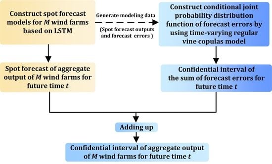
Figure 3 shows the interval forecasting method by using LSTM-TVRVC.

3.2. Evaluation Indices

Reliability and sharpness are two aspects of evaluating a forecasting interval [46]. Generally, reliability is the primary factor that needs to be guaranteed for interval forecasting, and the average coverage deviation (ACD) is a commonly used index for evaluating reliability. The nominal mean prediction interval width (NMPIW) is a commonly used index for evaluating sharpness.

For a given nominal confidence level $1-\alpha$, the formula of the ACD is as follows:

$$ACD=PICP-\left(1-\alpha \right)$$

(17)

where $\mathrm{PICP}$ is the probability that the test samples lie within the forecasting intervals at the given confidence level; PICP is calculated by:

$$PICP=\frac{1}{N}{\displaystyle \sum _{i=1}^N{\lambda }_i}$$

(18)

where ${\lambda }_i$ is an indicator variable that is defined as follows:

$${\lambda }_i=\left\{\begin{array}{ll}1& {\widehat{q}}_i^{\left(\alpha /2\right)}<x_i<{\widehat{q}}_i^{\left(1-\alpha /2\right)}\\ 0& otherwise\end{array}\right.$$

(19)

where ${\widehat{q}}_i^{\left(\alpha /2\right)}$ and ${\widehat{q}}_i^{\left(1-\alpha /2\right)}$ are the lower and upper boundaries of the forecasting intervals, respectively, and $x_i$ is the $i-\mathrm{th}$ test sample. Forecasting intervals with small absolute values of the ACD values are more reliable.

The formula of the NMPIW is as follows:

$$NMPIW=\frac{1}{RN}{\displaystyle \sum _{i=1}^N\left({\widehat{q}}_i^{\left(1-\alpha /2\right)}-{\widehat{q}}_i^{\left(\alpha /2\right)}\right)}$$

(20)

where N is the number of test samples and R is the difference between the maximum and minimum real wind power output values. Reliable forecasting intervals with smaller NMPIWs are preferred.

The skill score (SS) is a comprehensive index that considers both reliability and sharpness [37]; the SS is positively oriented and computed as follows:

$$SS=\frac{1}{N}{\displaystyle \sum _{i=1}^N{\displaystyle \sum _{j=1}^K\left({\xi }_i^{\left({\alpha }_j\right)}-{\alpha }_j\right)}\left(x_i-{\widehat{q}}_i^{\left({\alpha }_j\right)}\right)}$$

(21)

where ${\xi }_i^{\left({\alpha }_j\right)}$ is an indicator variable that equals 1 when $x_i\le {\widehat{q}}_i^{\left({\alpha }_j\right)}$ and that equals 0 otherwise. When K = 2, ${\alpha }_1=1-\frac{\alpha }{2}$ and ${\alpha }_2=\frac{\alpha }{2}$, (21) is the SS for the confidence level $1-\alpha$.

4. Results and Discussion

The proposed method is applied to three adjacent wind farms in Northwest China to verify its effectiveness. Each wind farm has an installed capacity of 50 MW, and the data resolution is 15 min. The distance between any two of the three wind farms is no more than 50 km, and Kendall’s tau coefficients for the real outputs of the three wind farms are shown in

Table 1. Kendall’s tau coefficients for the three wind farms.

	Wind Farm 1 and 2	Wind Farm 1 and 3	Wind Farm 2 and 3
Kendall’s tau coefficients	0.944	0.907	0.888

, demonstrating strong correlations.

The historical data of the three wind farms for the whole year of 2017 are divided into four datasets (datasets 1–4), and each dataset contains three months of wind power output data. The proposed method is applied to these four datasets to verify its effectiveness.

For each dataset, the training set of the spot forecasting model contains the historical data of the three wind farms over the first two months, and the test dataset contains the historical data of the third month. The modeling data for the TVRVC are the spot forecasting data and the forecasting error data of the three wind farms over the first three weeks of the third month (generated by the spot forecast model based on LSTM networks), and confidence intervals for the aggregate output of the fourth week of the third month are finally calculated to verify the validity of the interval forecast method.

4.1. Spot Forecasting Results and Discussion

The LSTM networks have two hidden layers with 32 and 8 hidden units, and the learning rate is set as 0.005. To conduct a comparison with the LSTM networks, a spot forecasting model based on BP neural networks is also created, and the modeling steps are the same as those in Section 3.1, only the LSTM networks are replaced by the BP networks. The BP networks also have two hidden layers with 32 and 8 hidden units, and the learning rate is set as 0.005. The root mean square error (RMSE) is taken as the evaluation index, and its formula can be found in [1]. The RMSEs of the two spot forecasting models are shown in

Table 2. RMSEs of different spot forecasting models.

		RMSE(MW)
		Dataset 1	Dataset 2	Dataset 3	Dataset 4
LSTM	Wind Farm 1	2.2742	2.3768	2.5133	2.1485
	Wind Farm 2	2.4184	2.4868	2.5812	2.2508
	Wind Farm 3	2.5702	2.7155	2.7471	2.4642
BP	Wind Farm 1	3.4114	3.5652	3.7699	3.2227
	Wind Farm 2	3.6276	3.7301	3.8717	3.3762
	Wind Farm 3	3.8554	4.0732	4.1206	3.6962

.

For each wind farm, the RMSE of the spot forecasting model based on the LSTM networks does not exceed 5% of the installed capacity and is smaller than that of the BP neural networks. The results demonstrate the effectiveness of the spot forecasting model used in this paper.

4.2. Structures of the Time-Varying Regular Vine Copulas for the Three Wind Farms

The structure of each tree and the type of bivariate copula model corresponding to each edge in the TVRVC of the three wind farms for dataset 1 are shown in Figure 4.

Table 3. AIC indices produced when fitting edge 1,2 and edge 5,2|1 with five types of copula functions.

	AIC (×103)
	Gaussian	t	Clayton	Gumbel	SJC
1,2	−6.105	−6.222	−8.204	−7.074	−7.673
5,2|1	−0.177	−0.306	−0.744	−0.163	−0.823

shows the AIC values produced when fitting edge 1,2 and edge 3,6|5 with five types of time-varying copula functions.

Table 3 shows that the optimal bivariate copula for edge 1,2 is the Clayton copula and for edge 5,2|1, it is the SJC copula.

4.3. Interval Forecasting Results and Discussion

Figure 5 shows the aggregate output intervals, the real aggregate output values and the spot-forecasted aggregate output values at different confidence levels for the three wind farms on days 1–2 of the fourth week of the third month in dataset 1.

As Figure 5 shows, the forecasting interval of the proposed method can effectively envelop the real aggregate output of the three wind farms and can reflect uncertainty characteristics well even when the real output fluctuates greatly. The figure also shows that the width of the interval is narrower when the wind power output is smaller and wider when the output is larger, which indicates that the uncertainty of the aggregate output of the three wind farms is smaller at lower wind power output levels.

Figure 6 shows the means and fluctuation ranges of the absolute values of the ACD for each of the four datasets at different confidence levels.

Regarding reliability, the means of the absolute values of the ACD indices obtained for the four datasets do not exceed 4% at all confidence levels and fluctuates within 3%. Regarding sharpness, the interval width of the 90% confidence interval is only 10% and fluctuates within 5%. The forecasting results show that the method proposed in this paper is highly adaptable, has good performance during different periods of the year and has small interval widths while remaining highly reliable.

The following methods are designed for comparison with the methods proposed in this paper:

• BP networks and time-varying regular vine copulas (BP-TVRVC) method: The forecast error data generated by BP networks are used for time-varying regular vine copulas modeling, and the RMSE of the BP networks is shown in Table 2.
• LSTM networks and time-varying copulas (LSTM-TVC) method: This is a superposition method. After performing spot forecasting with the LSTM networks, modeling the time-varying bivariate copula of the spot forecasting outputs and forecasting errors for each wind farm to obtain their respective forecasting intervals, the forecast intervals are superimposed as their aggregate output interval. This method ignores the spatial correlation between multiple wind farms.
• LSTM networks and static regular vine copulas (LSTM-SRVC) method: LSTM networks are still used for spot forecasting, but the time-varying copula functions used in the time-varying regular vine copula model are replaced by the corresponding static copula functions. This method considers the correlations among the outputs of multiple wind farms but does not consider the time-varying nature of the correlations; this method was also used in ref. [37].
• LSTM networks and time-varying regular vine Gaussian copulas (LSTM-TVRVGC) method: After the LSTM networks are used for the spot forecasting, the regular vine copula model is constructed with the time-varying Gaussian copulas. This method corresponds to the method used in [38].

The absolute values of the ACD, NMPIW and SS obtained by the method proposed in this paper and the four methods mentioned above are shown in Figure 7a,b and

Table 4. SSs of different interval forecast methods.

Nominal Confidence	SS
	LSTM-TVRVC	BP-TVRVC	LSTM-TVC	LSTM-SRVC	LSTM-TVRVGC
90%	−1.325	−1.984	−1.454	−1.504	−1.384
80%	−2.016	−2.998	−2.093	−2.211	−2.121
70%	−2.439	−3.728	−2.544	−2.705	−2.644
60%	−2.808	−4.273	−2.882	−3.051	−3.013
50%	−3.021	−4.694	−3.138	−3.292	−3.263
40%	−3.185	−4.995	−3.334	−3.444	−3.411
30%	−3.329	−5.201	−3.476	−3.524	−3.482
20%	−3.400	−5.328	−3.573	−3.554	−3.508
10%	−3.444	−5.395	−3.624	−3.566	−3.513
mean	−2.774	−4.288	−2.902	−2.983	−2.927

, respectively. For presentation purposes, the index scores in Figure 7a,b and Table 4 are the mean index scores of the forecasting intervals obtained for the four datasets.

Comparing the proposed method with the BP-TVRVC method, the absolute values of the ACDs of both methods are less than 6% at all confidence levels, thus indicating that these two methods are both reliable. Since the absolute values of the ACDs of these two methods are small and do not differ significantly, more attention is given to sharpness. As Figure 7b shows, the method proposed in this paper has smaller NMPIW values, thus indicating that using a spot forecasting model with a small error in combination with the copula model helps improve the sharpness of the forecast interval.

Comparing the proposed method with the LSTM-TVC method, the NMPIW values of the LSTM-TVC method are smaller than those of the proposed method at all confidence levels, thus indicating that the former method has higher sharpness. However, in terms of reliability, the absolute values of the ACDs of the LSTM-TVC method are greater than those of the proposed method at all confidence levels, especially at 90% confidence levels. The values of the ACD of the LSTM-TVC method are 4 times as large as those of the proposed method, thus indicating that considering the spatial correlation of multiple wind farms is beneficial to compensating for the single wind farm forecasting errors, thus improving the reliability of the forecasting intervals. Although the sharpness of the LSTM-TVC method is higher, its reliability, which is the most important for interval forecasting, is not as good as that of the method proposed in this paper.

Comparing the proposed method with the LSTM-SRVC method, the absolute value of the ACDs of the proposed method are smaller than that of the LSTM-SRVC method at all confidence levels, thus indicating that the proposed method has higher reliability. Additionally, the absolute values of the ACDs of the proposed method do not vary much; with a minimum value of 0.982% at the 10% confidence level and a maximum value of 3.087% at the 30% confidence level, the difference between the maximum and minimum values is 2.117%, while the absolute values of the ACDs of the methods using static copula functions vary greatly at different confidence levels, with a minimum value of 3.325% at the 90% confidence level and a maximum value of 16.723 at the 40% confidence level. The difference between the maximum and minimum values is 13.398%. This result indicates that it is difficult to accurately capture the correlations of multiple wind farms and maintain high reliability at different confidence levels by using static copula functions that ignore the time-varying characteristics of the correlations. Regarding sharpness, the NMPIW values of the proposed method at all confidence levels are smaller than those of the LSTM-SRVC method. Figure 8 shows the forecasting intervals of the LSTM-SRVC method for days 1–2 of the fourth week of the third month in dataset 1.

Comparing Figure 8 with Figure 5 shows that the forecasting intervals can effectively envelop the real aggregate wind power regardless of whether static copula functions or time-varying copula functions are used, but the width of the intervals produced by the method using static copula functions is significantly larger than that of the proposed method, indicating that the forecasting result of the LSTM-SRVC method are more conservative.

Comparing the proposed method with the LSTM-TVRVGC method, the absolute values of the ACDs of the LSTM-TVRVGC method are larger than those of the proposed method at all confidence levels, and the values of the ACDs vary greatly at different confidence levels. This indicates that it is also difficult to accurately model the correlation of multiple wind farms and achieve high reliability at different confidence levels by using only one type of copula function. In terms of sharpness, the NMPIW values of the proposed method are smaller than those of the LSTM-TVRVGC method at all confidence levels.

In terms of the comprehensive index, the SS values of the proposed method are closer to 0 than those of the other four methods, thus indicating that the proposed method has the best overall performance.

5. Conclusions

This paper proposes an interval forecasting method by combining a spot forecast model based on LSTM networks and a time-varying regular vine copula model. Case analysis shows that the proposed method can provide high-reliability forecast intervals with reasonable interval widths.

In the case study, comparing the proposed method with the method using only a single type of copulas, the method using static copulas (which thus ignores time-varying characteristic of correlations among multiple wind farms), and the superposition method (which thus ignores spatial correlations among multiple wind farms), the results show that the proposed method strikes a good balance between reliability and sharpness and has good comprehensive performance because of consideration of the temporal and spatial correlation of multiple wind farms and the use of multiple types of copula functions. Furthermore, the copula model was combined with a different spot forecasting model to interval forecasting in the case analysis, and the result shows that a spot forecasting model with smaller errors leads to sharper forecasting intervals.

In conclusion, by combining a spot forecast model with a small error and an improved copula model that considers the temporal and spatial correlation of multiple wind farms, the proposed method can provide accurate uncertain information on wind power for scheduling plans, thus improving the economic benefit and reliability of the system operation. Future research will focus on how to further improve spot forecast accuracy and apply the interval forecast result to scheduling decisions.

References

- Zhou, B.; Ma, X.; Luo, Y.; Yang, D. Wind Power Prediction Based on LSTM Networks and Nonparametric Kernel Density Estimation. IEEE Access 2019, 7, 165279–165292. [Google Scholar] [CrossRef]
- Zhao, C.; Wan, C.; Song, Y. Operating Reserve Quantification Using Prediction Intervals of Wind Power: An Integrated Probabilistic Forecasting and Decision Methodology. IEEE Trans. Power Syst. 2021, 36, 3701–3714. [Google Scholar] [CrossRef]
- He, Y.; Li, H. Probability density forecasting of wind power using quantile regression neural network and kernel density estimation. Energy Convers. Manag. 2018, 164, 374–384. [Google Scholar] [CrossRef]
- Haque, A.U.; Nehrir, M.H.; Mandal, P. A Hybrid Intelligent Model for Deterministic and Quantile Regression Approach for Probabilistic Wind Power Forecasting. IEEE Trans. Power Syst. 2014, 29, 1663–1672. [Google Scholar] [CrossRef]
- Wan, C.; Lin, J.; Wang, J.; Song, Y.; Dong, Z.Y. Direct Quantile Regression for Nonparametric Probabilistic Forecasting of Wind Power Generation. IEEE Trans. Power Syst. 2016, 32, 2767–2778. [Google Scholar] [CrossRef]
- Yu, Y.; Yang, M.; Han, X.; Zhang, Y.; Ye, P. A Regional Wind Power Probabilistic Forecast Method Based on Deep Quantile Regression. IEEE Trans. Ind. Appl. 2021, 57, 4420–4427. [Google Scholar] [CrossRef]
- Zhou, M.; Wang, B.; Guo, S.; Watada, J. Multi-objective prediction intervals for wind power forecast based on deep neural networks. Inf. Sci. 2020, 550, 207–220. [Google Scholar] [CrossRef]
- Wan, C.; Zhao, C.; Song, Y. Chance Constrained Extreme Learning Machine for Nonparametric Prediction Intervals of Wind Power Generation. IEEE Trans. Power Syst. 2020, 35, 3869–3884. [Google Scholar] [CrossRef]
- Xu, Q.; He, D.; Zhang, N.; Kang, C.; Xia, Q.; Bai, J.; Huang, J. A Short-Term Wind Power Forecasting Approach with Adjustment of Numerical Weather Prediction Input by Data Mining. IEEE Trans. Sustain. Energy 2015, 6, 1283–1291. [Google Scholar] [CrossRef]
- Safari, N.; Chung, C.Y.; Price, G.C.D. Novel Multi-Step Short-Term Wind Power Prediction Framework Based on Chaotic Time Series Analysis and Singular Spectrum Analysis. IEEE Trans. Power Syst. 2017, 33, 590–601. [Google Scholar] [CrossRef]
- Bizrah, A.; Almuhaini, M. Modeling wind speed using probability distribution function, Markov and ARMA models. In Proceedings of the IEEE Power & Energy Society General Meeting, Denver, CO, USA, 26–30 July 2015; pp. 1–5. [Google Scholar]
- Ekanayake, P.; Peiris, A.T.; Jayasinghe, J.M.J.W.; Rathnayake, U. Development of Wind Power Prediction Models for Pawan Danavi Wind Farm in Sri Lanka. Math. Probl. Eng. 2021, 2021, 4893713. [Google Scholar] [CrossRef]
- Ibrahim, M.; Alsheikh, A.; Al-Hindawi, Q.; Al-Dahidi, S.; ElMoaqet, H. Short-Time Wind Speed Forecast Using Artificial Learning-Based Algorithms. Comput. Intell. Neurosci. 2020, 2020, 8439719. [Google Scholar] [CrossRef] [PubMed]
- Akbal, Y.; Ünlü, K.D. A univariate time series methodology based on sequence-to-sequence learning for short to midterm wind power production. Renew. Energy 2022, 200, 832–844. [Google Scholar] [CrossRef]
- Farah, S.; David, A.W.; Humaira, N.; Aneela, Z.; Steffen, E. Short-term multi-hour ahead country-wide wind power prediction for Germany using gated recurrent unit deep learning. Renew. Sustain. Energy Rev. 2022, 167, 112700. [Google Scholar] [CrossRef]
- Abualigah, L.; Abu Zitar, R.; Almotairi, K.H.; Hussein, A.M.; Elaziz, M.A.; Nikoo, M.R.; Gandomi, A.H. Wind, Solar, and Photovoltaic Renewable Energy Systems with and without Energy Storage Optimization: A Survey of Advanced Machine Learning and Deep Learning Techniques. Energies 2022, 15, 578. [Google Scholar] [CrossRef]
- Zhang, Y.; Chen, B.; Zhao, Y.; Pan, G. Wind Speed Prediction of IPSO-BP Neural Network Based on Lorenz Disturbance. IEEE Access 2018, 6, 53168–53179. [Google Scholar] [CrossRef]
- Tian, W.; Bao, Y.; Liu, W. Wind Power Forecasting by the BP Neural Network with the Support of Machine Learning. Math. Probl. Eng. 2022, 2022, 7952860. [Google Scholar] [CrossRef]
- Yang, L.; He, M.; Zhang, J.; Vittal, V. Support-Vector-Machine-Enhanced Markov Model for Short-Term Wind Power Forecast. IEEE Trans. Sustain. Energy 2015, 6, 791–799. [Google Scholar] [CrossRef]
- Yuan, X.; Chen, C.; Jiang, M.; Yuan, Y. Prediction interval of wind power using parameter optimized Beta distribution based LSTM model. Appl. Soft Comput. 2019, 82, 105550. [Google Scholar] [CrossRef]
- Yuan, C.; Tang, Y.; Mei, R.; Mo, F.; Wang, H. A PSO-LSTM Model of Offshore Wind Power Forecast considering the Variation of Wind Speed in Second-Level Time Scale. Math. Probl. Eng. 2021, 2021, 2009062. [Google Scholar] [CrossRef]
- Santhosh, M.; Venkaiah, C.; Kumar, D.V. Short-term wind speed forecasting approach using Ensemble Empirical Mode Decomposition and Deep Boltzmann Machine. Sustain. Energy Grids Netw. 2019, 19, 100242. [Google Scholar] [CrossRef]
- Yan, J.; Li, K.; Bai, E.-W.; Deng, J.; Foley, A.M. Hybrid Probabilistic Wind Power Forecasting Using Temporally Local Gaussian Process. IEEE Trans. Sustain. Energy 2015, 7, 87–95. [Google Scholar] [CrossRef]
- Kou, P.; Gao, F.; Guan, X.; Wu, J. Prediction intervals for wind power forecasting: Using sparse warped Gaussian process. In Proceedings of the 2012 IEEE Power and Energy Society General Meeting, San Diego, CA, USA, 22–26 July 2012; pp. 1–8. [Google Scholar] [CrossRef]
- Yang, H.; Yuan, J.; Zhang, T. A model and algorithm for minimum probability interval of wind power forecast errors based on Beta distribution. Proc. CSEE 2015, 35, 2135–2142. [Google Scholar] [CrossRef]
- Lan, F.; Sang, C.; Liang, J.; Li, J. Interval prediction for wind power based on conditional Copula function. Proc. CSEE 2016, 36, 79–86. [Google Scholar] [CrossRef]
- Quan, H.; Khosravi, A.; Yang, D.; Srinivasan, D. A Survey of Computational Intelligence Techniques for Wind Power Uncertainty Quantification in Smart Grids. IEEE Trans. Neural Netw. Learn. Syst. 2019, 31, 4582–4599. [Google Scholar] [CrossRef] [PubMed]
- Davidson, M.R.; Zhang, D.; Xiong, W.; Zhang, X.; Karplus, V.J. Modelling the potential for wind energy integration on China’s coal-heavy electricity grid. Nat. Energy 2016, 1, 16086. [Google Scholar] [CrossRef]
- Kang, C.; Yao, L. Key scientific issues and theoretical research framework for power systems with high proportion of renewable energy. Autom. Electr. Power Syst. 2017, 41, 2–11. [Google Scholar]
- Peng, X.; Chen, Y.; Cheng, K.; Wang, H.; Zhao, Y.; Wang, B.; Che, J.; Liu, C.; Wen, J.; Lu, C.; et al. Wind Power Prediction for Wind Farm Clusters Based on the Multifeature Similarity Matching Method. IEEE Trans. Ind. Appl. 2020, 56, 4679–4688. [Google Scholar] [CrossRef]
- Andrade, J.R.; Bessa, R.J. Improving Renewable Energy Forecasting with a Grid of Numerical Weather Predictions. IEEE Trans. Sustain. Energy 2017, 8, 1571–1580. [Google Scholar] [CrossRef]
- Lobo, M.G.; Sanchez, I. Regional Wind Power Forecasting Based on Smoothing Techniques, With Application to the Spanish Peninsular System. IEEE Trans. Power Syst. 2012, 27, 1990–1997. [Google Scholar] [CrossRef]
- Peng, X.; Xiong, L.; Wen, J.; Cheng, S.; Wang, B. A Summary of the State of the Art for Short-term and Ultra-short-term Wind Power Prediction of Regions. Proc. CSEE 2016, 36, 6315–6326. [Google Scholar] [CrossRef]
- Zhang, N.; Kang, C.; Xia, Q.; Liang, J. Modeling Conditional Forecast Error for Wind Power in Generation Scheduling. IEEE Trans. Power Syst. 2014, 29, 1316–1324. [Google Scholar] [CrossRef]
- Alexiadis, M.; Dokopoulos, P.; Sahsamanoglou, H. Wind speed and power forecasting based on spatial correlation models. IEEE Trans. Energy Convers. 1999, 14, 836–842. [Google Scholar] [CrossRef]
- Yunus, K.; Chen, P.; Thiringer, T. Modelling spatially and temporally correlated wind speed time series over a large geographical area using VARMA. IET Renew. Power Gener. 2016, 11, 132–142. [Google Scholar] [CrossRef]
- Wang, Z.; Wang, W.; Liu, C.; Wang, Z.; Hou, Y. Probabilistic Forecast for Multiple Wind Farms Based on Regular Vine Copulas. IEEE Trans. Power Syst. 2017, 33, 578–589. [Google Scholar] [CrossRef]
- Duan, S.; Miao, S.; Lixing, L.I.; Han, J.; Qingyu, T.U.; Yaowang, L.I. Uncertainty Model of Combined Output for Multiple Wind Farms Considering Dynamic Correlation of Prediction Errors. Autom. Electr. Power Syst. 2019, 43, 31–37. [Google Scholar]
- Nelsen, R.B. An Introduction to Copulas; Springer: Berlin/Heidelberg, Germany, 2006. [Google Scholar] [CrossRef]
- Kurowicka, D.; Joe, H. Dependence Modeling: Vine Copula Handbook; World Scientific: Singapore, 2010. [Google Scholar] [CrossRef]
- Attoh-Okine, N. Copula Models. In Big Data and Differential Privacy; John Wiley & Sons: Hoboken, NJ, USA, 2017; pp. 175–195. [Google Scholar] [CrossRef]
- Patton, A.J. Modelling Time-Varying Exchange Rate Dependence Using the Conditional Copula. SSRN Electron. J. 2001. [Google Scholar] [CrossRef]
- Patton, A.J. On the Out-of-Sample Importance of Skewness and Asymmetric Dependence for Asset Allocation. J. Financ. Econ. 2004, 2, 130–168. [Google Scholar] [CrossRef]
- Shahid, F.; Zameer, A.; Muneeb, M. A novel genetic LSTM model for wind power forecast. Energy 2021, 223, 120069. [Google Scholar] [CrossRef]
- Hossain, M.A.; Chakrabortty, R.K.; Elsawah, S.; Gray, E.; Ryan, M.J. Predicting Wind Power Generation Using Hybrid Deep Learning with Optimization. IEEE Trans. Appl. Supercond. 2021, 31, 1–5. [Google Scholar] [CrossRef]
- Dong, W.; Sun, H.; Tan, J.; Li, Z.; Zhang, J.; Yang, H. Regional wind power probabilistic forecasting based on an improved kernel density estimation, regular vine copulas, and ensemble learning. Energy 2022, 238, 122045. [Google Scholar] [CrossRef]
Figure 1.
A possible structure of the six-dimensional regular vine copulas.
Figure 2.
Flow chart for modeling the conditional joint PDF of the forecasting errors for multiple wind farms by TVRVC.