Article

Evolutionary Process for Engineering Optimization in Manufacturing Applications: Fine Brushworks of Single-Objective to Multi-Objective/Many-Objective Optimization

1
College of Information Science and Engineering, Northeastern University, Shenyang 110819, China
2
Key Laboratory of Data Analytics and Optimization for Smart Industry, Ministry of Education, Shenyang 110819, China
3
Frontier Science Center for Industrial Intelligence and System Optimization, Ministry of Education, Shenyang 110819, China
*
Authors to whom correspondence should be addressed.
These authors contributed equally to this work.
Processes 2023, 11(3), 693; https://doi.org/10.3390/pr11030693
Submission received: 10 January 2023 / Revised: 9 February 2023 / Accepted: 19 February 2023 / Published: 24 February 2023
(This article belongs to the Special Issue Evolutionary Process for Engineering Optimization (II))

Abstract

:
Single-objective to multi-objective/many-objective optimization (SMO) is a new paradigm in the evolutionary transfer optimization (ETO), since there are only “1 + 4” pioneering works on SMOs so far, that is, “1” is continuous and is firstly performed by Professors L. Feng and H.D. Wang, and “4” are firstly proposed by our group for discrete cases. As a new computational paradigm, theoretical insights into SMOs are relatively rare now. Therefore, we present a proposal on the fine brushworks of SMOs for theoretical advances here, which is based on a case study of a permutation flow shop scheduling problem (PFSP) in manufacturing systems via lenses of building blocks, transferring gaps, auxiliary task and asynchronous rhythms. The empirical studies on well-studied benchmarks enrich the rough strokes of SMOs and guide future designs and practices in ETO based manufacturing scheduling, and even ETO based evolutionary processes for engineering optimization in other cases.

1. Introduction

Single-objective to multi-objective/many-objective optimization (SMO) is conveyed in a “Big K Tree” (Figure 1b) by our groups of DAO and IIAIAO, which derives from a Chinese lantern (Figure 1a).
As Chinese lanterns symbolize red ornaments for a festive atmosphere, the Chinese lantern regarding SMOs in Figure 1 is dedicated to the establishment of our lab, Frontier Science Center for Industrial Intelligence and System Optimization (FSCIIASO), Ministry of Education from 2021, which is a national level center. In FSCIIASO, we emphasize the key word of “system optimization” (SO, SO is also in the name of FSCIIASO) when designing an SMO framework [1,2,3,4].
In the lantern, “eMeets” presents big pictures of three “where to go” strategies for SMOs, which serve as rough strokes of SMOs (the old version is [5], our new version of [5] is submitted with the new title of “Evolutionary Transfer Optimization Meets Manufacturing: Single-objective to Multi-objective/Many-objective Optimization for ‘Taiji’ ”). The follow-up studies of “eMeets” are “rMeets” and “iMeets”. “iMeets” are fine brushworks of SMOs.
Start our scientific journey of “iMeets” with deep learning (to a great extent, the tide of interpretability is set off by deep learning), a popular kind of black box based artificial intelligence (AI) [1,2,3,4,5,6,7,8,9,10,11,12,13,14,15,16,17,18,19,20,21,22,23,24,25,26,27,28,29,30,31,32,33,34,35,36,37,38,39,40,41]. In the deep learning community, many researchers endeavor to open the black box via universality, generalizability [19], over-parametrization and so on.
For example, in the [1] paper “A proposal on machine learning via dynamical systems”, an applied and computational mathematician uses a powerful mathematical tool of dynamical system towards a better characterization of deep neural network models.
Then, time for interpretability [30,40] of the computational models in ETOs, which also belongs to black box based AI [29]. According to the problem types, the paradigm [3] of ETOs includes five kinds, two of which are the following: (1) An ETO for multi-task optimization (MTO) and (2) ETO for complex optimization. As a subset of (2), single-objective to multi-objective/many-objective optimization (SMO) is new. To date there are only “1 + 4” works on SMOs, “1” is performed by [10], where they firstly invented an SMO, and “4” was proposed by DAO and IIAIAO (names of our groups).
Theoretical insights into an ETO, which belongs to complex systems [42,43,44,45,46,47,48,49,50,51,52,53,54,55,56,57,58,59,60,61,62,63,64] and system optimization [2,31,36,37] problems are relatively rare, whether for an MTO or for an SMO.
Finally, let us take a closer look at both an MTO and an SMO for an ETO interpretability as follows:
For MTOs and interpretability: In [55], they propose a general formalization of an ETO and introduce a classification of three categories, sequential transfer, multitasking and multiform optimization. In [56], they investigate the theoretical studies guaranteeing a faster convergence when compared to the case of a conventional single task. To analyze the effects of information transferred from related tasks, they first propose a novel multi-task gradient descent (MTGD) algorithm, which enhances the updates of a standard gradient descent with a term of multi-task interaction. They derive the convergence of the MTGD and present the first proof of a faster convergence of the resultant MTGD relative to its counterpart of a single task. Via the MTGD, they formulate an evolutionary multitasking algorithm that is gradient-free, which is called a multi-task evolution strategy (MTES). Additionally, the single task evolution strategy (ES) they use is shown to approximate the gradient descent asymptotically and extends the faster convergence results derived for the case of the MTGD to the MTES as well. Numerical experiments comparing the MTES with the case of a single task ES on synthetic benchmarks and real work examples substantiate their theoretical claim.
For SMOs and interpretability: Here come our four surgical knives on search/convergence landscapes, i.e., building blocks, transfer gaps, auxiliary tasks and asynchronous rhythms, for a whole picture/proposal of interpretability for an SMO “meeting” the permutation flow shop scheduling problem (PFSP) towards the manufacturing scheduling (MS) and carbon neutrality. Because opening the black boxes is somehow similar to treating an illness or having an operation we call our lenses on landscapes above as surgical knives. In “iMeets”, we will focus on the abstract SMO implemented with a genetic algorithm (GA) and a memetic algorithm (MA) to disentangle the knowledge for many industrial applications (Notes: 1. It should be highlighted that the SMO is general and abstract, which can be realized by many special algorithms; 2. The PFSP is also an abstract model in computer networking, beyond its original modelling of shop scheduling, showing inherent wide applications. Therefore, we say “many industrial applications”). Although the ES above differs from our MA, both of them do share some common insights within a common language of exploration and exploitation (“R-IT”) balance.
Main contributions are as follow:
  • To the best of our knowledge, it is the first attempt to extend a proposal of interpretability on an SMO “meeting” the PFSP towards disentangling the knowledge for smart manufacturing scheduling and carbon neutrality.
  • We further extend the classical building block hypothesis within the ETO learning settings to confirm the existence of positional building blocks (BB) [7,8,9,24,25,26,27] in whole chromosomes, whether head, middle or tail (the first surgical knife of a building block).
  • We characterize the landscapes in different gaps towards a proper guarantee of a correlation gap and an asynchronous rhythm (the second and fourth surgical knives of transfer gaps and asynchronous rhythms).
  • We further discuss the gather [6] or transfer coefficient between the auxiliary tasks for boosting the core task. (The third surgical knife of the auxiliary task).
The related works are as follows: Interpretability via transfer optimization (TO) (for the ease of discussion below, TO is exchangeable with ETO here) towards the opening of a black box. Moreover, the TO and other black box based AIs [51,52,53,54,55,56,57,58,59,60], includes machine learning (ML). One of the most popular subsets of ML is deep learning (DL). In the following, we will discuss four groups of related works within eight related papers, some of which are quite important and inspiring.
Interpretable TO for a continuous case (similar to our ETO_PFSP) and vehicle routing: Firstly, to their best knowledge, their paper is the first work of an evolutionary multi-objective optimization [13] to enhance the optimization by knowledge transferred from corresponding single-objective problems. [10] In the deep analysis part of the IV.B in their work, they put that the transfer success rate has a positive correlation with the paradigm efficacy, which can be applied to guide the adaptive conduction of a knowledge transfer towards a positive transferring. Secondly, in paper [12] of a TO based vehicle routing, they investigate key theoretical questions of knowledge memes, such as “How do the knowledge memes of related problem domain affect the evolutionary search?” and “What forms of knowledge memes from related problem domains benefit evolutionary optimization”. However, those insights are for vehicle routing, not shop scheduling.
Interpretable DL on landscapes of empirical risk in both discriminative and generative cases: First of all, here is a paper [57] for a discriminative case. The most successful DL models for vision, such as VGG and ResNets are best used when a degree of “over-parametrization” is equipped. In this work, they characterize the landscape of the empirical error of over-parametrized DL models. Then, in another [58] attempt (conducted by one of the authors of this paper, Wendi Xu) follows the landscape work above, extending the discriminative case to generative case via a case study of image super resolution from both biological and mathematical sides.
Interpretable DL for unsupervised and transfer learning: Begins with paper [59], we find that the general-purpose priors for representation learning includes 10 examples: (1) smoothness, (2) multiple explanatory factors, (3) a hierarchical organization of explanatory factors, (4) semi-supervised learning, (5) shared factors across tasks, (6) manifolds, (7) natural clustering, (8) temporal and spatial coherence, (9) sparsity and (10) simplicity of factor dependencies. They try to “disentangle” several “of the underlying (and a priori unknown) factors of variation that the data may reveal”. Moreover, the paper [53] answers “why unsupervised pre-training of representation can be useful” and how it can be used for transfer learning.
Interpretable ML via a dynamical system and a weak mechanism from computation-al and an applied mathematics community: In paper [1] of “a proposal on machine learning via dynamic systems”, the author provide an attractive alternative view of a continuous dynamic system to DL, with a well modeling of a general high-dimensional nonlinear function used in machine learning. Another source of mathematical insight is a lens of weak mechanism, proposed by a professor in the forum [61] held by the Beijing Academy of Artificial Intelligence (BAAI).
In the following, we organize the presentation in a straightforward way. Section 2 gives the specific problem for an evolutionary process for an engineering optimization in manufacturing applications, that is a PFSP, and the targeted methods in the SMO abstract framework. Then, after the preparation of a problem application and tool framework, we show their interaction in Section 3, that is the empirical settings and computational running/simulating. With vivid analogies and interesting descriptions in Section 3, we show four insights and the whole picture or proposal is made up of them in Section 4. At last, conclusions in Section 5 serves as the “take home messages” and also say more about the lantern and the labs. Additionally, embracing deep learning is on the way for future works there.

2. Materials and Methods

2.1. Test Problem: PFSP

In many manufacturing systems, all jobs must undergo a series of machine operations. Often, these machine operations have to be performed on each job in the same processing order, implying that each job has to follow the same processing route. The machines are then assumed to be in a series and the scheduling environment is referred to as a setting of a flow shop. Usually, each queue [33] is assumed to process under the rule of First In First Out (FIFO) discipline, that is, all jobs cannot “pass” another job while waiting for processing in a arranged queue. If the discipline of the FIFO is in effect, the flow shop production system is referred to as a setting of a permutation flow shop. Therefore [33], the scheduling problem in a permutation flow shop is named PFSP. Therefore, the PFSP [16,35,38] is formulated as follows: each job or operation is to be arranged sequentially on corresponding machines, given their own processing time of the machine operation [49]. Every machine can process one operation or job at most, and every job can be processed at most on one machine during optimization. The sequence of job permutation is the same on every machine.
The feasibility [32] of search spaces or solution spaces in a PFSP is due to the corresponding satisfaction of the optimization constraints (in scheduling problems, a high level of feasibility usually means a low level of sparseness in solution spaces and vice versa). Relatively less optimization constraints in the nature of the PFSP will simplify the problems (more complicated cases, such as job shop) or discrete problems in real world applications, whose solution spaces may be broken up by temporal type restrictions on tasks and/or jobs or resources and/or machines, making the traversal of the solution spaces quite confounded. Thus, the PFSP, which also has the building blocks that are straightforward, could serve as a nice starting point/platform [64,65] for the investigation into the scheduling applications or discrete problems, which may be extended for reentrant scheduling problems.
The optimality [32] of the search space or solution space is due to the corresponding satisfaction of the optimization objectives. As to the optimization objectives in cases of the PFSP, we chose the objectives of makespan (Cmax) and total flow time (TFT) as goals towards optimality for production management. Real-world industrial problems for manufacturing systems lead to intractable model sizes when rigorous mathematical formulations are carefully used, which motivates and encourages our evolutionary style of SMOs that enjoy a happy medium between a good enough solution quality and a tolerable time cost.

2.2. The Framework across Tasks: ETO_PFSP or SMO

2.2.1. Four Frameworks: SOO, MOO, MFO and SMO

As in the paper [44], there are three types of optimization problems, that is, single-objective optimization (SOO), multi-objective optimization (MOO) and multi-factorial optimization (MFO). The SMO here is nearly the same as the MOO, aiming to boost the core task, and shares some common transferring mechanisms with MFO. Our ETO_PFSP is the first discrete case of an SMO.

2.2.2. 4 Bags, 4 × 2 Groups, 4 × 2 × 4 tasks: e.g., Bag 0: Group 1, t1_wc(t_wc 1.0, t_wc 1.1), t2_wc and t2e_wc; Group 2, t1_nc(t_nc 1.0, t_nc 1.1), t2_nc and t2e_nc

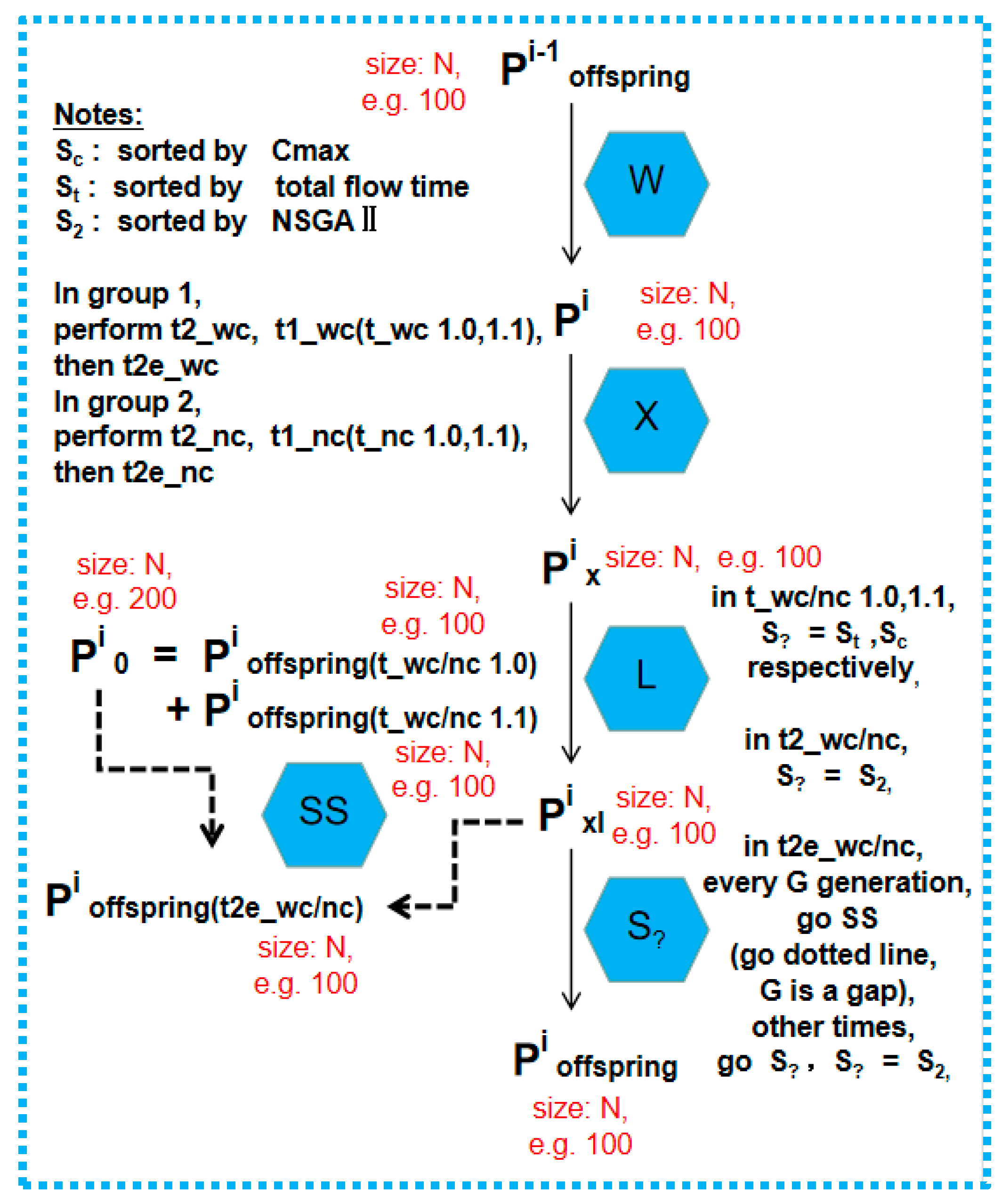
The overview is in Figure 2. In ETO_PFSP, for each Bag, we setup two task groups.
Bag 0 is full of group 1 and group 2. “Group 1 has four optimization tasks, namely, task t1_wc, including two sub tasks (task t_wc 1.0 and task t_wc 1.1), task t2_wc and task t2e_wc, where “wc” is with clustering and “e” means external transferring from task t1_wc, sharing the same optimization toolkit of W-X-L (only cross probabilities vary in X, more can be seen in 3.1). All of the above are the same as in group 2 of task t1_nc (task t_nc 1.0 and task t_nc 1.1), task t2_nc and task t2e_nc, except that no clustering (named “nc”) is in operator W [49]. For Bag 0, each case calculates the measure of the hamming distance in the job permutation from the whole chromosome (that is, head, middle and tail).
Bag 5 owns groups 3 and 4, which are nearly the same as group 1 and group 2 in Bag 0. Only two settings differ. First, M modification is set in groups 3 and 4 to obtain the former two, that is, just remove M(M) in X. Secondly, in bag 5, each case calculates the measure of the hamming distance in the job permutation from head, middle to tail, separately (just test the special distribution of positional BB).
Then, Bag 6 stores group 5 and 6, which are also nearly the same as group 1 and 2. Only two setups differ. M modification is set. Moreover, there is just a change to the transferring gaps.
Moving forward with Bag 7, which is occupied by groups 7 and 8, which are nearly the same as groups 1 and 2. Only add two new settings. M modification is used and testing the different combinations of the transfer coefficients in the auxiliary tasks.
Lastly, we achieve Bag 8 (groups 9 and 10), which are nearly the same as groups 1 and 2, with an addition of two new settings. M modification is applied. and the testing of the different asynchronous rhythms.
W-X-L deploys a special operator to choose parents (W), a crossover (X) operator and a local search (L) operator. It is worth mentioning that the family of tasks above shares the same initial (I) population(random) for a fair comparison. The phase of selection (S) differs. For S, we use NSGAII, some sorting methods by the Cmax objective or TFT objective and so on. Therefore, there are so many shared parts above from both the problem and algorithm sides, which are elaborately constituted towards a harmony test bed for a well-defined SMO.
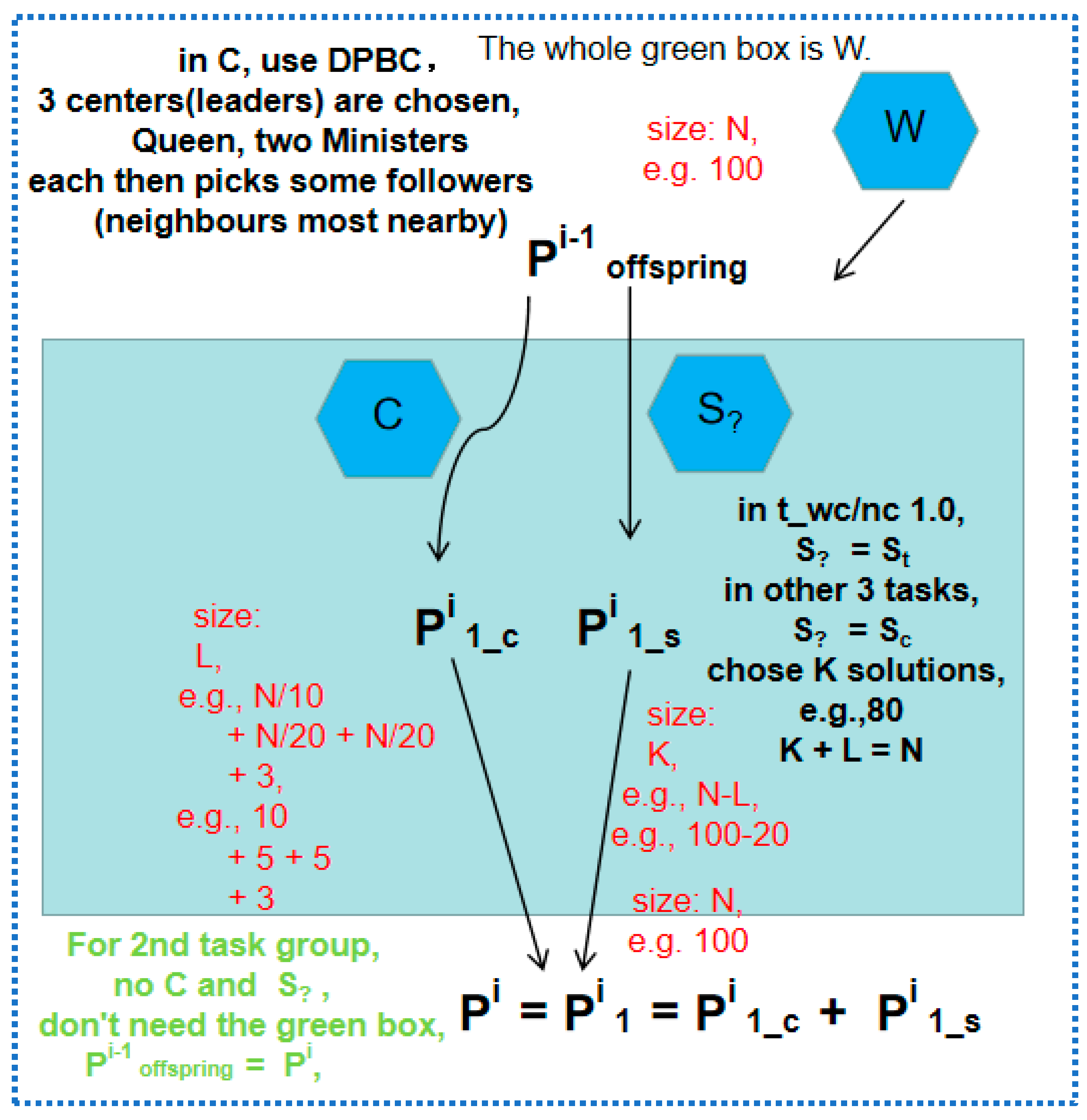
The details of W (seen in Figure 3). For W, with C and S? (Figure 4), we choose parents Pi. The key component, density peak based clustering (DPBC) [54] is developed in C.
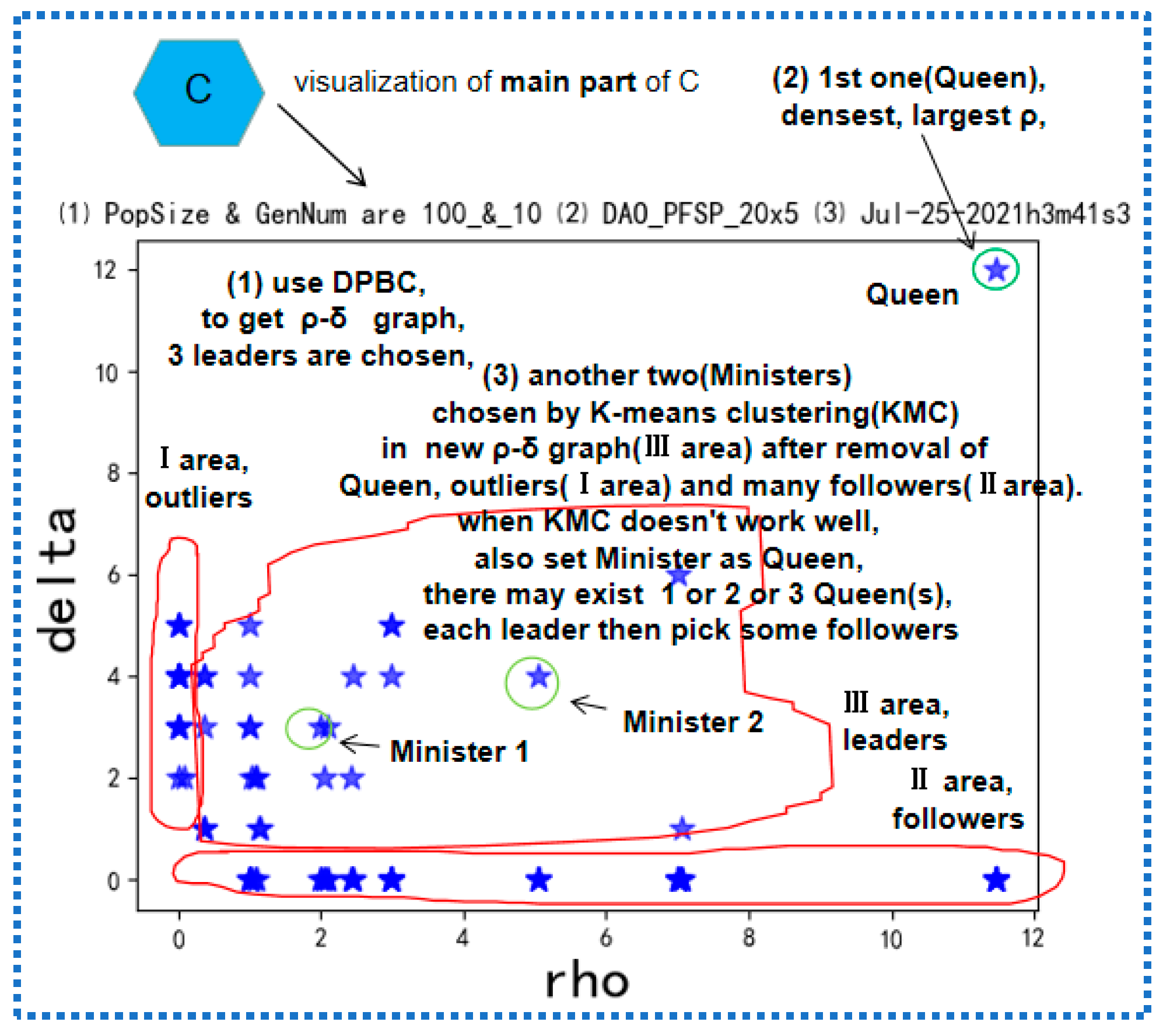
Here is the detail of C. In [54], “science clustering” (because it was published at journal of “science”, so we call it “science clustering”) is based on the deep observation that the centers of clusters in a sample space are characterized by both “a relatively higher density than points in their neighborhoods” [6,49] and “a relatively long distance from points that have higher densities” [6,49]. For the PFSP here, we implement science clustering via a hamming distance metric, which is widely accepted and used in evolutionary computation research. To our surprise, the hamming distance also focuses on the work of mining the positional BBs. Quite obviously and intuitively, the measure of the “hamming distance (dissimilarity) and positional BB (similarity) work from opposite sides to the same characterization” [6,49].
The details of XL (in Figure 5), especially X. More of X is in Figure 5. L is an ordinary insertion operator.
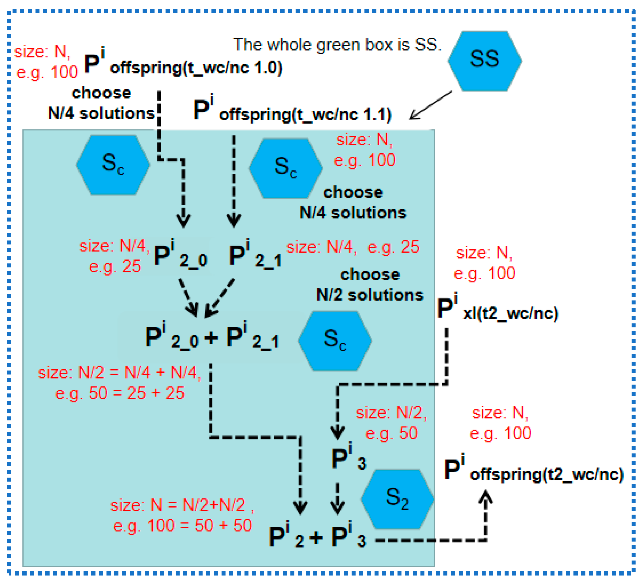
The details of SS in S (seen in Figure 6). Both task t1_wc/nc and task t2_wc/nc have no settings of Pi0, only task t2e_wc/nc needs the setting of Pi0 every G generation [49]. Both task t_wc/nc 1.0 and 1.1 establish the selection pressure via the settings of a single optimization objectives, and both tasks t2_wc/nc and t2e_wc/nc use both the optimization objectives via the NSGAII.

3. Results

3.1. Experimental Setup

To test the validation of the SMO or the framework of the ETO_PFSP, we carry out an extensive computational simulation on some well-known PFSP instances in well-studied international benchmarks, that is, instance tai01(20 × 5), instance tai42 (50 × 10) and instance VFR100_20_1(100 × 20), e.g., the simple symbol of 20 × 5, denotes 20 jobs and five processing machines in the PFSP.
And in our computational simulation, ETO_PFSP or SMO is run on computer servers.
The following simulation parameters of the SMO are set: “N is set as 100, and the number of generations is set as 100. In task t1_wc/nc 1.0 and 1.1, [px1, px2/m] are set as [0.3, 0.7] and [0.1, 0.9], respectively. For task t2_wc/nc and task t2e_wc/nc, i is the value of [0.2, 0.8]. For options of reference points, instance tai01 takes the range of (2500, 1000) to normalize the optimization objective of Cmax, and (25,000, 10,000) to normalize the optimization objective of TFT; instance tai42 uses the values of (4200, 2500) and (120,000, 80,000); and instance three picks the settings of (10,000, 5000) and (550,000, 350,000). The G gap chooses 2. The base-line size of Pi2 is given as 50, which is modified by a factor of K1. For the size of Pi1, the base-line size takes 20 + H. Additionally, 20 above is also adapted by a value of K2, H can be 0, 1, 2 or 3, depending on the computational solutions with equally measured distances at a corresponding cutting distance [49].
Varying the setup of [K1, K2] in each Bag in 4.2 (The setting is a vector of [1, 0.6] in Bags 5, 6 and 7. While, for Bag 8, the vector is [1,1]), we obtain nine cases (in Figure 7, Figure 8, Figure 9 and Figure 10, each figure owns nine cases) for Bags 5 or 6 or 7 or 8, and each case owns a total of 20 independent runs. In each run, we perform computational simulations of eight optimization tasks, that is, two optimization task groups.

3.2. Simulations and Comparisons

In every case, both task t2_wc and task t2e_wc work with clustering, and both task t2_nc and task t2e_nc are performed without clustering.
In every case, we evolve overall 4 (bags) × 100 (generations per task) × 4 (4 tasks in each group) × 2 (wc/nc, that is wc or nc) × 20 (independent runs) = 80,000 generations.
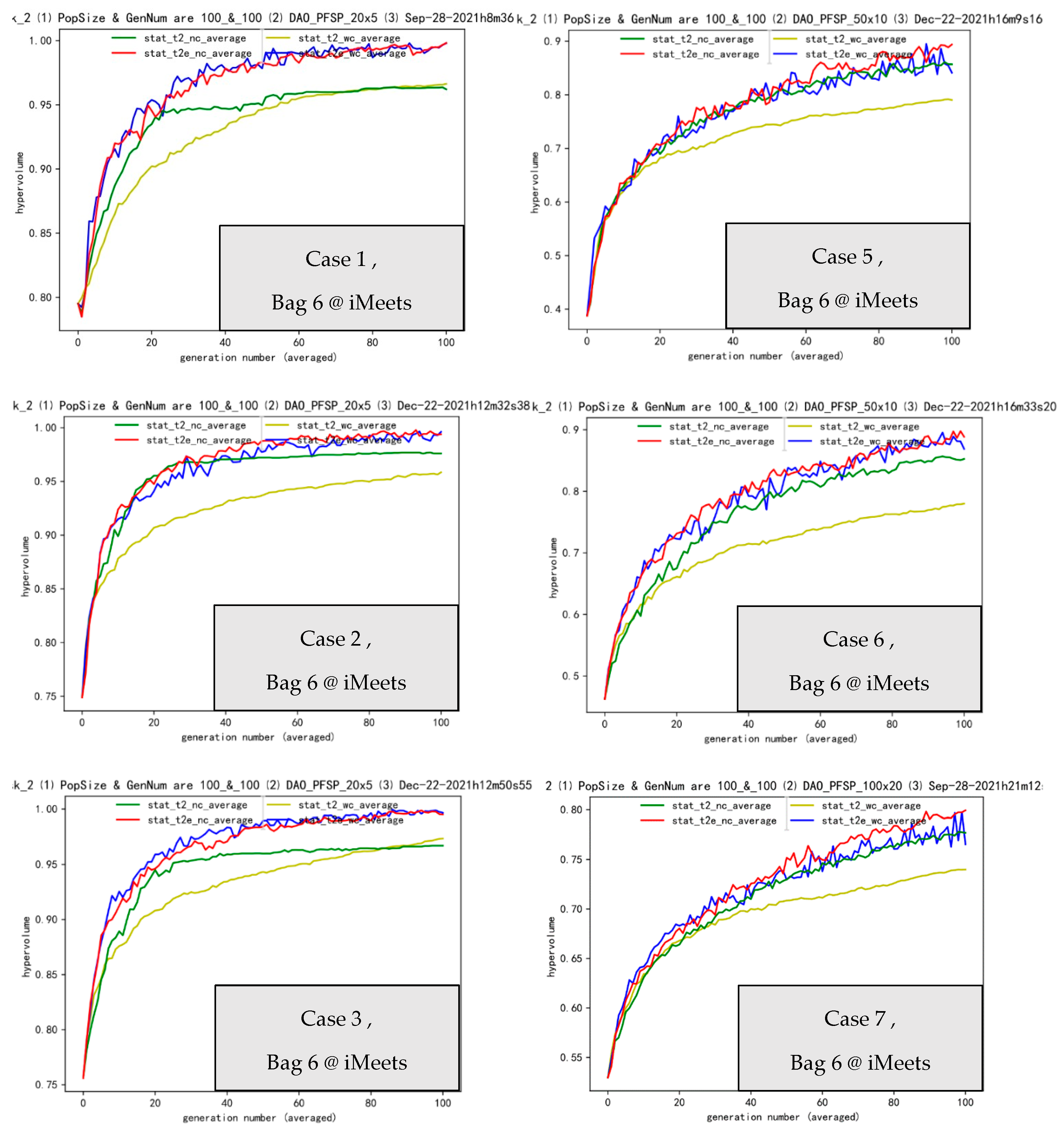
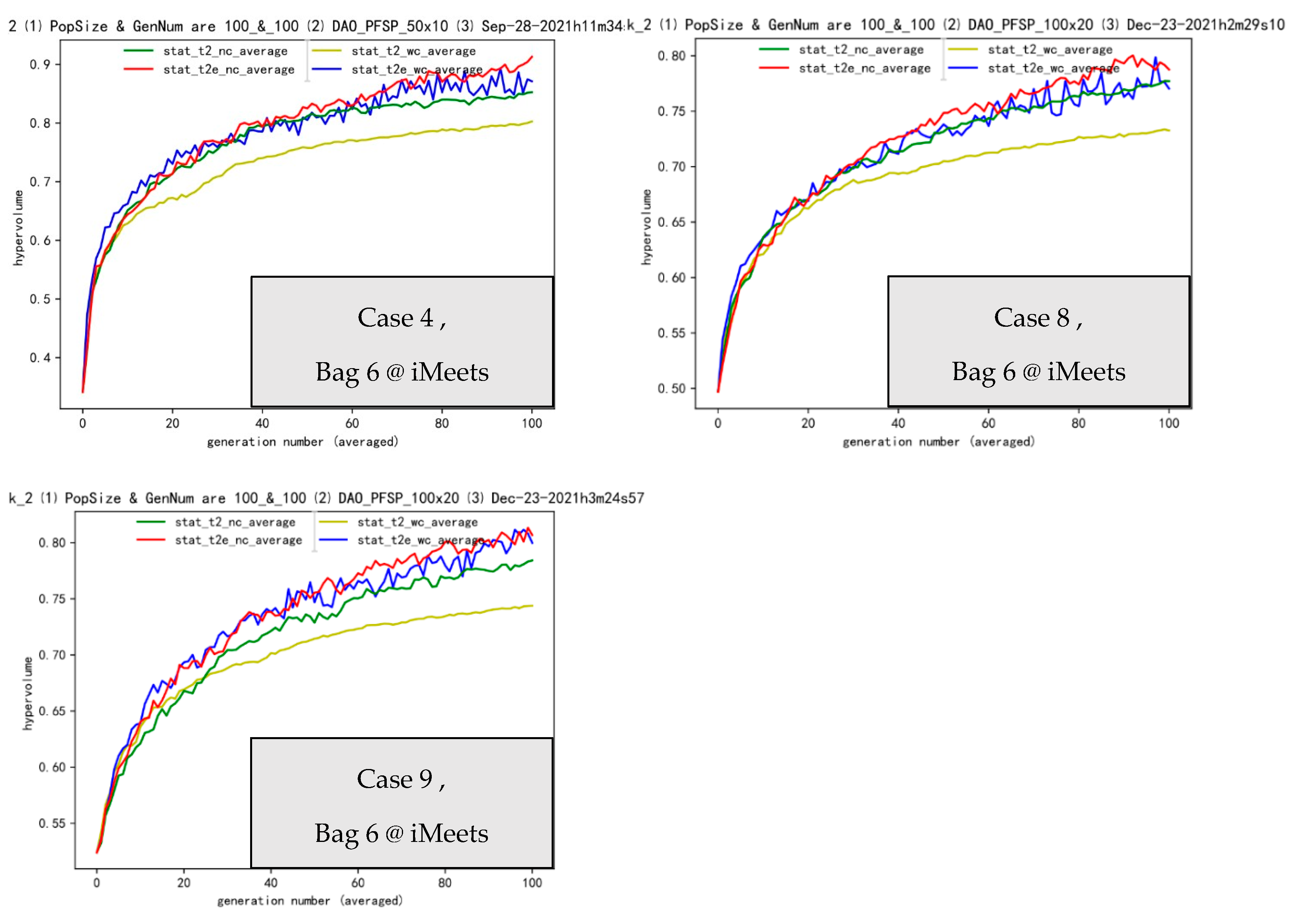
Then, in Bags 5, 6, 7 and 8 (Figure 7, Figure 8, Figure 9 and Figure 10), we will give a more systematic study of each facet/lens, then combine the four facets to obtain the whole picture/proposal.
For Bag 5, we test the lens/surgical knife of building block distribution.
A vivid intention or original design of Bag 5 is to find the specific contribution of each section.
For example, we may expect that the tail section in the chromosome contributes mostly and acts as the main driving power, which will shadow and hide the middle section and the tail section.
If we find that cases 1 and 2 give results of very low effective transferring, that is to say, the distance among the two lines that we are interested in in Figure 7 are too close to each other, while searching for dynamic results in case 3, tell us that there is a very encouraging and obvious positive transferring effectiveness is discovered or that an improvement in the distance from the source line to the target line that we care about in Figure 7 is large, then we will be more confident to give prominence to the main role of the tail section.
However, from Figure 7, we do not find that anyone in the three sections conquers the other two.
For to Bag 5, between t2_wc and t2e_wc pair, there is almost always (except case eight) an obvious positive transferring effectiveness in Figure 6 (a figure containing nine results), which tends to validate that there exists a great effectiveness in the part in of the SMO. Whereas, as to t2_nc and t2e_nc, both great effectiveness and normal effectiveness exist. Those are in Table 1 below.
Then, in Bag 6 below, we will focus on the facet on transfer gaps/rhythms. Here are another nine cases as follows:
An interesting idea and a vivid analogy of Bag 6 is that someone may tend to walk quickly and some may become accustomed to a slow style of walking.
We should find the most suitable way and the best working statue for an SMO’s transfer gap setting, therefore we compare four persons in each case in Figure 8 below.
There are 4 × 9 = 36 persons attempt to find their most comfortable working styles.
As to Bag 6, between the pair of t2_wc and t2e_wc, there is definitely an obvious positive transferring effectiveness in Figure 9 above, which tends to validate a great effectiveness (ee) part in our framework.
Whereas, for t2_nc and t2e_nc, both normal effectiveness (e) and ineffectiveness (ie) can be seen.
Those two observations are summed up below in Table 2.
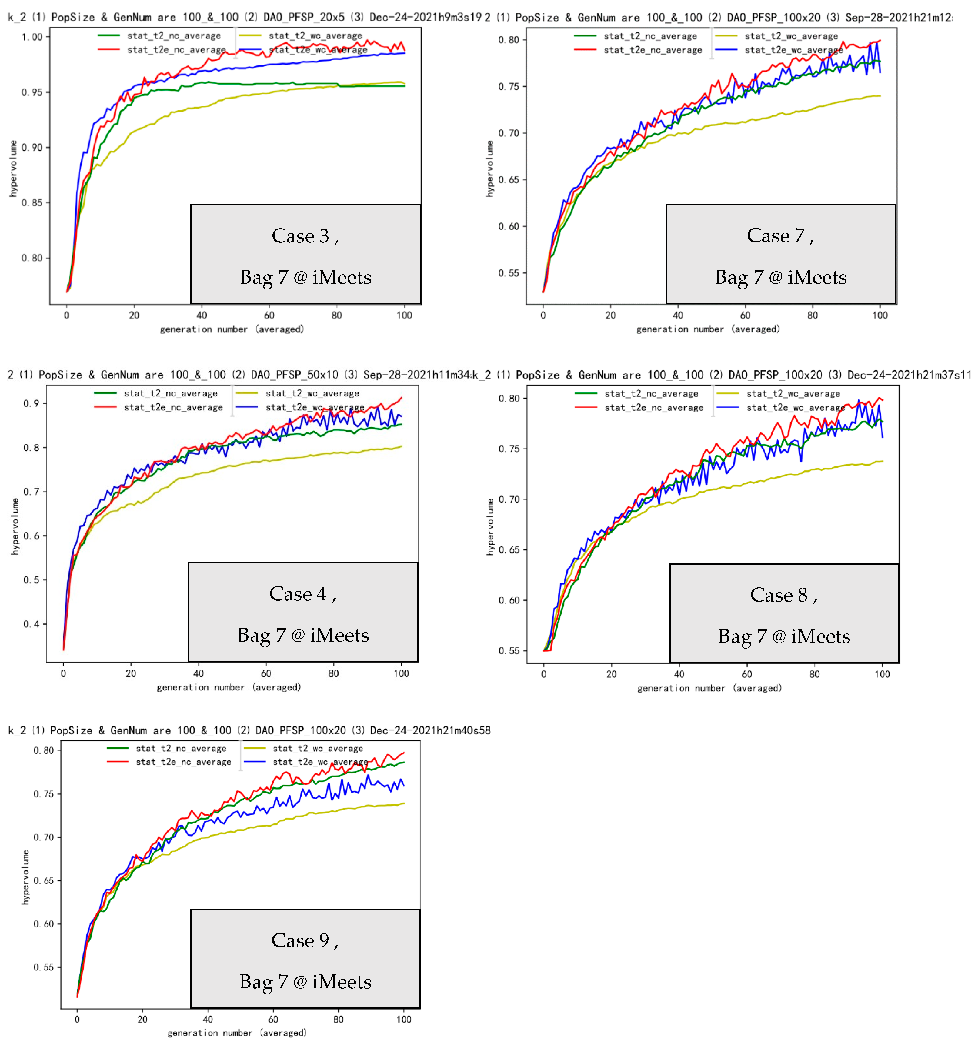
Then, moving forward to Bag 7 below, we will just study the lens of the transfer coefficient.
A helpful imagination of Bag 7 is that one leader may have two assistants (task t_wc 1.0 and task t_wc 1.1) and he is not clear about which assistant is more suitable or stronger for him.
For instance, the left assistant of the TFT objective, that is task t_wc 1.0, may give more supporting strength than the right one or task t_wc 1.1.
And in Bag 7, between the tasks of t2_wc and t2e_wc, or between the pair of t2_nc and t2e_nc, and an obvious positive transferring effectiveness exists in Figure 10, which tends to strongly validate the great effectiveness (ee) in the SMO.
Those observations are again summed up via Table 3.
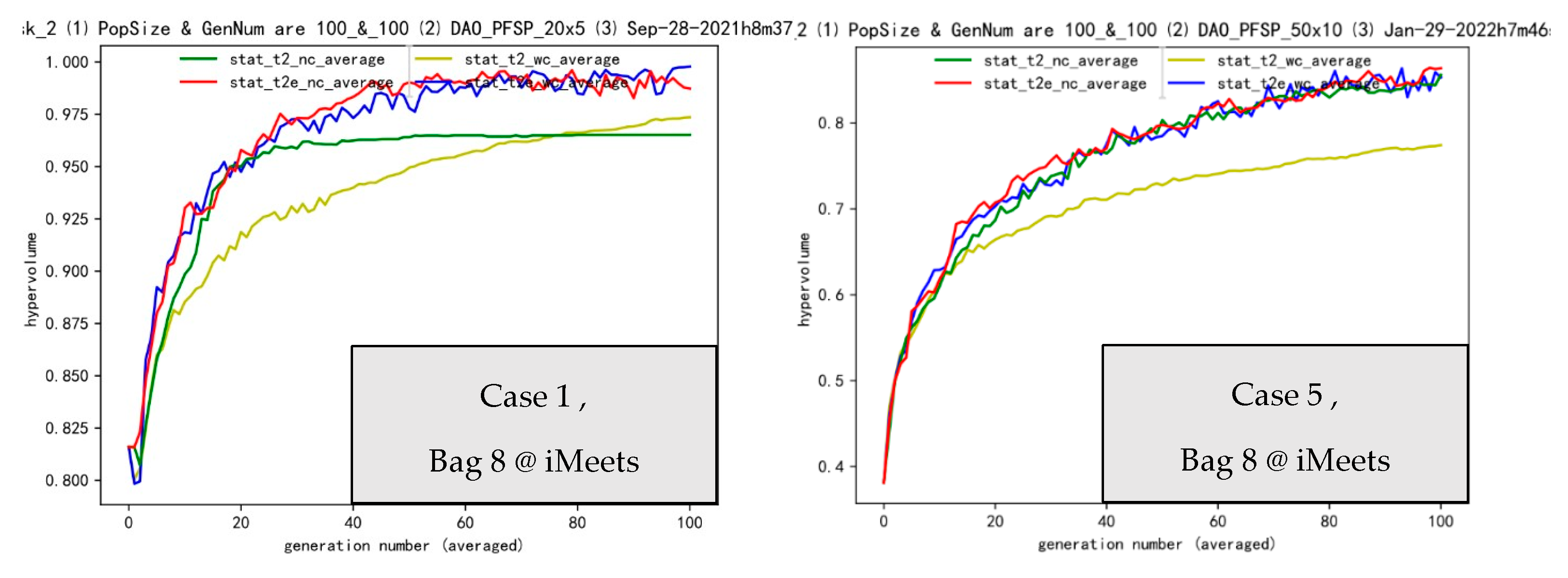
Then, in Bag 8 below, we will take a closer look at the surgical knife of the asynchronous gaps/rhythms. Another nine cases are as follows.
A strong motivation behind Bag 8 is our intuitive sense of music. Why should the gap be equal for both sides (task t_wc 1.0 and task t_wc 1.0)? If the balance is lost, what will happen? Equal rhythm is necessary? In a managerial background, people are not satisfied with intuitive observation; therefore, our investigation of Bag 8 in Figure 10 is striking for those questions.
In Bag 8, for the tasks of t2_wc and t2e_wc, there is both normal effectiveness (e) and great effectiveness (ee) in Figure 10 above, which tends to validate the effectiveness part in the SMO.
Whereas, between t2_nc and t2e_nc, normal effectiveness (e), great effectiveness (ee) and ineffectiveness (ie) can be seen.
Those are summed up below in Table 4.

4. Discussion

4.1. Insight into Bag 5: Building Block Distribution in Head, Middle and Tail

The BB theory/hypothesis is mainly based on Goldberg’s decomposition theory, which contains seven steps as follow: (1) “Know what GAs process”—BBs; (2) solve the optimization problems, which have bounded the BB difficulty; (3) ensure that the supply of raw BBs is adequate; (4) ensure that the “market share” of superior BBs increases; (5) know “BB takeover” and the models of the convergence times; (6) ensure that GAs make the BB decisions well; and (7) ensure that the mixing of BBs is good.
According to those seven steps, the BB processing pipelines with five steps are as follows: (1) creation, which creates the raw supply of BBs; (2) identification, that attempts to identify the good BBs; (3) separation, which separates the superior BBs; (4) preservation, which maintains the good BBs; and (5) mixing, that reassembles good BBs [21].
Considering these “7 + 5” steps above and transferred knowledge, we propose a hypothesis that a positional BB dominates other BBs. Let us study Cmax. For Makespan or Cmax, the minimum result of the maximum completion time plays the role of the most powerful and core optimization objective/driving force among the management objectives in many-objective, multi-objective and single-objective machine scheduling problems. Cmax dominates the total flow time (TFT), maximum lateness, total tardiness and so on. In other words, it should be put forward first that better a Cmax, usually, is also strongly correlated with other better optimization objectives. For combinational problems, especially for machine scheduling or a PFSP, those building blocks remains unclear and some important clues may help us. Positional, precedent and adjacent types of information units in combinational problems are believed to exist. In travel salesman problems, positional structures are dominated by adjacency structures, while positional structures matter more than adjacency structures for the optimization objective of Cmax in the case of the PFSP [27]. Based on those observations above, we tend to believe that there may exist three kinds of BBs, that is, positional, precedent and adjacent BBs. In experiments here, we will focus on the first one, the positional BB. Therefore, we can summarize that BBs of a positional type help improve the Cmax, and also improve other objectives inherently, the significance of positional ones is highlighted here.
According to the discussions above, Bag 5 tends to tell us that positional building blocks are located everywhere, no matter in the head, middle or tail. Problems with specified structures and/or known building block distributions may help solve the question better. So in the future, we need PFSP datasets, such as ImageNet to build transparent models and paradigms, constituting a well-defined search space topology [38].

4.2. Insight into Bag 6: Fitness Landscape Analysis via Gaps 2, 4 and 1

Fitness landscape analysis [39,41] gives insight into the reactions between algorithms and problems, and provide the measurement of correlations between tasks. The tool or model of the local optima network (LON) may help explain the meta-heuristic search dynamics. Because our instance is large (20, 50 and 100), not in the current tractable scope of LON (in job shop scheduling, the pattern of instance difficulty is “easy-hard-easy”, we also tend to believe that the scope here is beyond the relatively easy instances in LON research now), we still analyze the landscape via a straightforward hv-generation picture in Bag 6. We changed the key factor of the transferring gaps from 2 and 4, to 1.
Comparing gap 2 with 4, without a clustering setting (a dark green line and a red line), the boosting between tasks is nearly lost. Partly due to the loss of correlation in the fitness landscapes. However, for gaps 2 and 4, with the clustering setting (a light green line and a blue line), the correlation still exists, although weakened by the new setting. Therefore, a larger gap should be cautious.
Comparing gaps 2 and 1, without clustering, the boosting effectiveness between the tasks remains because of the existence of the correlation conveyed in the fitness landscape. Additionally, for gaps 2 and 4, with clustering, the correlation still comes. Therefore, a closer gap is allowed.

4.3. Insight into Bag 7: Auxiliary Tasks, Transfer Coefficient and Driving Forces

From Bag 7, we find that the boosting effectiveness between the light green line and the blue line is the lowest in each triple (case 1, 2 and 3, triple 1; cases 4, 5 and 6, triple 2; and cases 7, 8 and 9, triple 3).
That is, 2*task 1.1(mm, cases 3, 6 and 9) is the worst combination of the transfer coefficients [56], and 1×task 1.0 + 1×task 1.1(tm, case 1, 4, 7) and 2×task 1.0(tt, case 2, 5 and 8) are nearly the same. (In MTES [56], the authors also care about the transfer coefficients, which inspires our work here via the common framework of “R-IT” balance.)
Both auxiliary tasks (mm, case 3, 6 and 9) via makespan, will decrease the diversity in the solution space; therefore, this harms the performance because the auxiliary tasks will be greatly covered by the domination of the makespan driving force (4.1 already discusses makespan) in the core tasks.

4.4. Insight into Bag 8 and the Whole Picture/Proposal Combining Bag 5,6,7,8: Asynchronous Rhythm, 3W Framework

In each triple (cases 1, 2 and 3, triple 1; cases 4, 5 and 6, triple 2; and cases 7, 8and 9, triple 3) of Bag 8, the order of the boosting or the transferring performance between t2_wc and t2e_wc regarding the asynchronous rhythms is: “222” > “424” > “422”.
The first “>” agrees with the insight into Bag 6, an improper slower rhythm or larger gap harms the SMO (that is, four is slower and the larger, or two is better than four).
Additionally, the second “>”, tells us that one asymmetric aesthetics (“422”. For “22” or “44”, we say symmetric aesthetics, while “24” or “42” is asymmetric aesthetics.) does not play more sounder music than the two asymmetric aesthetics (“424”), although one gap (gap 2), which is smaller or faster (“422” owns an additional right 2 than “424”). The two asymmetric aesthetics still hold the balance of the total symmetric aesthetics. Engineering, science and art (or music) agree on the same rule defined/conquered by Nature/Truth/Gold.
After we gather insights into Bags 5, 6, 7 and 8, let us try to obtain the whole picture/proposal. As Prof. Yao Xin from Southern University of Science and Technology puts (in a forum about the interpretability topic held by the Tencent Research Institute on the 11 January 2022), interpretability faces a key and common framework of 3W, that is, Who, What and Why.
Here, to our researchers (Who), the proposal (What) of “keep eyes on the whole chromosome, be cautious of larger gaps, encourage diverse auxiliary tasks and asynchronous asymmetric rhythms whilst still preferring to hold on to the total symmetric/balance of music” are the potential important tips to explain why SMOs work well. For people who are less familiar with our evolutionary and learning tools, the proposal should be different and more specified.

5. Conclusions

Heading towards the international pledge of China’s carbon neutrality [16] and implementing “system optimization” scientific pursuits in both DAO/FSCIIASO and IIAIAO (DAO is Key Laboratory of Data Analytics and Optimization for Smart Industry, Ministry of Education, and IIAIAO is Institute of Industrial Artificial Intelligence And Optimization. Both D.H. and W.X. are also from IIAIAO.), we need powerful SMOs. To develop and apply powerful SMOs, we need SMO interpretability or SMO insights.
Our SMO insights are in a proposal: “keep eyes on the whole chromosome, be cautious of larger gaps, encourage diverse auxiliary tasks and asynchronous asymmetric rhythms whilst still preferring to hold onto the total symmetric/balance of music”. The proposal attempts to answer the questions of disentangling the knowledge for both theoretical and practical demands. There is both science and art (the fourth insight, with some connections with music or rhythms) in SMOs.
From both theoretical and practical sides, we tend to believe that transfer coefficients, transfer gaps and transfer core (so far, in the SMO, the operator SS is the core) are key concepts for SMOs and ETOs.
In the future, many directions [38,53], are inspiring and attractive. To build surrogates armed with deep learning [14,15,17,18,23,28,50] in SMO seems important. Combining interpretability in both deep learning and SMOs may open the black boxes in complex systems and boost the scientific advances for “system optimization” in “tai ji” [2].

Author Contributions

Conceptualization, D.H., X.W., Q.G. and W.X.; methodology, R.Z., X.S. and G.Z.; software, W.X., X.S. and G.Z.; validation, R.Z., X.S. and G.Z.; formal analysis, W.X., X.S. and G.Z.; investigation, Y.Y., T.X. and G.Z.; resources, Y.Y., T.X. and G.Z.; data curation, Y.Y., T.X. and G.Z.; writing—original draft preparation, W.X. and G.Z.; writing—review and editing, D.H., X.W., Q.G., R.Z., X.S. and W.X.; visualization, Y.Y., T.X. and G.Z.; supervision, D.H., X.W., Q.G., Y.Y., R.Z. and T.X.; project administration, D.H. and X.W.; funding acquisition, X.W., D.H. and Q.G. All authors have read and agreed to the published version of the manuscript.

Funding

This research was supported by the National Natural Science Foundation of China (72101052), the National Key Research and Development Program of China (2021YFC2902403).

Data Availability Statement

Data available on request from the authors.

Acknowledgments

We thank He Dakuo for great financial supports. We thank Teacher Zhou Han (also, in our group of DAO, NEU) for her useful support and kindly help. Xu Wendi also thanks Li Zuocheng (also, in our group), for his useful discussion of building block theory. Xu Wendi expresses his thank to Chen Yingping (from National Yang Ming Chiao Tung University) for his insights on linkage learning genetic algorithms, which helps him (Xu Wendi) understand the building block theory better. At last, authors thank reviewers and editor office of Processes for supportive help and key improvement.

Conflicts of Interest

The authors declare no conflict of interest.

References

  1. Weinan, E. A proposal on machine learning via dynamical systems. Comm. Math Stat. 2017, 5, 1–11. [Google Scholar]
  2. Tang, L.; Meng, Y. Data analytics and optimization for smart industry. Front. Eng. Mana. 2021, 8, 157–171. [Google Scholar] [CrossRef]
  3. Tan, K.; Feng, L.; Jiang, M. Evolutionary transfer optimization—A new frontier in evolutionary computation research. IEEE Comp. Inte. Magn. 2021, 16, 22–33. [Google Scholar] [CrossRef]
  4. Xu, W.; Zhang, M. Towards WARSHIP: Combining brain-inspried computing of RSH for image super resolution. In Proceedings of the 2018 5th IEEE International Conference on Cloud Computing and Intelligence Systems, Nanjing, China, 23–25 November 2018. [Google Scholar]
  5. Xu, W.; Wang, X.; Guo, Q.; Song, X.; Zhao, R.; Zhao, G.; Yang, Y.; Xu, T.; He, D. Towards KAB2S: Learning key knowledge from single-objective problems to multi-objective problem. arXiv 2022, arXiv:2206.12906. [Google Scholar]
  6. Xu, W.; Wang, X.; Guo, Q.; Song, X.; Zhao, R.; Zhao, G.; Yang, Y.; Xu, T.; He, D. Gathering strength, gathering storms: Knowledge Transfer via Selection for VRPTW. Mathematics 2022, 10, 2888. [Google Scholar] [CrossRef]
  7. Harik, G. Learning Gene Linkage to Efficiently Solve Problems of Bounded Difficulty Using Genetic Algorithms. Ph.D. Thesis, The University of Michigan, Ann Arbor, MI, USA, 1997. [Google Scholar]
  8. Chen, Y. Extending the Scalability of Linkage Learning Genetic Algorithms. In Part of the Studies in Fuzziness and Soft Computing Book Series; Springer: Berlin/Heidelberg, Germany, 2006. [Google Scholar]
  9. Chang, P.; Huang, W.; Wu, J.; Cheng, T. A block mining and recombination enhanced genetic algorithm for the permutation flow-shop scheduling problem. Inter. J. Prod. Econ. 2013, 141, 45–55. [Google Scholar] [CrossRef]
  10. Huang, L.; Feng, L.; Wang, H.; Hou, Y.; Liu, K.; Chen, C. A preliminary study of improving evolutionary multi-objective optimization via knowledge transfer from single-objective problems. In Proceedings of the 2020 IEEE International Conference on Systems, Man, and Cybernetics (SMC), Toronto, ON, Canada, 11–14 October 2020. [Google Scholar]
  11. Yuan, Y.; Ong, Y.; Gupta, A.; Tan, P.; Xu, H. Evolutionary multitasking in permutation-based combinatorial optimization problems: Realization with TSP, QAP, LOP, and JSP. In Proceedings of the 2016 IEEE Region 10 Conference (TENCON), Singapore, 22–25 November 2016. [Google Scholar]
  12. Feng, L.; Ong, Y.; Lim, M.; Tsang, I. Memetic search with interdomain learning: A realization between CVRP and CARP. IEEE Trans. Evol. Comp. 2015, 19, 644–658. [Google Scholar] [CrossRef]
  13. Wang, X.; Tang, L. A machine-learning based memetic algorithm for the multi-objective permutation flowshop scheduling problem. Comp. Oper. Rese. 2017, 79, 60–77. [Google Scholar] [CrossRef]
  14. Li, Y.; Wang, C.; Gao, L.; Song, Y.; Li, X. An improved simulated annealing algorithm based on residual network for permutation flow shop scheduling. Comp. Inte. Sys. 2020, 7, 1173–1183. [Google Scholar] [CrossRef]
  15. Shi, J.; Zhao, L.; Wang, X.; Zhao, W.; Huang, M. A novel deep Q-learning-based air-assisted vehicular caching scheme for safe autonomous driving. IEEE Trans. Intelli. Transport. Sys. 2020, 22, 4348–4358. [Google Scholar] [CrossRef]
  16. Wang, L.; Wang, J.; Wu, C. Advances in green shop scheduling. Control. Decis. 2018, 33, 385–391. [Google Scholar]
  17. Lei, N.; Luo, Z.; Yau, S.; Gu, D. Geometric understanding of deep learning. arXiv 2018, arXiv:1805.10451 2018. [Google Scholar] [CrossRef]
  18. Bronstein, M.; Bruna, J.; Cohen, T.; Velikovi, P. Geometric deep learning: Grids, groups, graphs, geodesics, and gauges. arXiv 2021, arXiv:2104.13478. [Google Scholar]
  19. Zhu, Y.; Gao, T.; Fan, L.; Huang, S.; Edmonds, M.; Liu, H.; Gao, F.; Zhang, C.; Qi, S.; Wu, Y.; et al. Dark, beyond deep: A paradigm shift to cognitive ai with humanlike common sense. arXiv 2020, arXiv:2004.09044 2020. [Google Scholar] [CrossRef]
  20. Wu, F.; Yang, C.; Lan, X.; Ding, J.; Zheng, N.; Gui, W.; Gao, W.; Chai, T.; Qian, F.; Li, D.; et al. Artificial intelligence: Review and future opportunities. Bull. Nation. Natur. Scie. Foun. China 2018, 32, 243–250. [Google Scholar]
  21. Li, D. Ten questions for the new generation of artificial intelligence. CAAI Trans. Intell. Sys. 2020, 15. [Google Scholar] [CrossRef]
  22. Littman, M.; Ajunwa, I.; Berger, G.; Boutilier, C.; Currie, M.; Velez, F.; Hadfield, G.; Horowitz, M.; Isbell, C.; Kitano, H.; et al. Gathering Strength, Gathering Storms: The One Hundred Year Study on Artificial Intelligence (AI100) Study Panel Report. Stanford University, Stanford, CA, USA, September 2021. Available online: http://ai100.stanford.edu/2021-report (accessed on 10 February 2023).
  23. Stone, P.; Brooks, R.; Brynjolfsson, E.; Calo, R.; Etzioni, O.; Hager, G.; Hirschberg, J.; Kalyanakrishnan, S.; Kamar, E.; Kraus, S.; et al. Artificial Intelligence and Life in 2030. Available online: http://ai100.stanford.edu/2016-report (accessed on 10 February 2023).
  24. Chen, Y.; Chuang, C.; Huang, Y. Inductive linkage identification on building blocks of different sizes and types. Inter. J. Syste. Scien. 2014, 43, 2202–2213. [Google Scholar] [CrossRef]
  25. Krasnogor, N.; Smith, J. A tutorial for competent memetic algorithms: Model, taxonomy and design issues. IEEE Trans. Evol. Comput. 2005, 9, 474–488. [Google Scholar] [CrossRef]
  26. Yazdani, D.; Cheng, R.; Yazdani, D.; Branke, J.; Jin, Y.; Yao, X. A survey of evolutionary continuous dynamic optimization over two decades—Part B. IEEE Trans. Evol. Comput. 2021, 49, 205–228. [Google Scholar]
  27. Cotta, C.; Fernández, A. Memetic Algorithms in Planning, Scheduling, and Timetabling; Springer: Berlin/Heidelberg, Germany, 2007. [Google Scholar]
  28. Deb, K.; Agrawal, S. Understanding interactions among genetic algorithm parameters. Found. Genet. Algorithms 2002, 5, 265–286. [Google Scholar]
  29. Al-Sahaf, H.; Bi, Y.; Chen, Q.; Lensen, A.; Mei, Y.; Sun, Y.; Tran, B.; Xue, B.; Zhang, M. A survey on evolutionary machine learning. Journ. Royal. Soci. N. Z. 2021, 49, 205–228. [Google Scholar] [CrossRef]
  30. Yu, Y.; Chao, Q.; Zhou, Z. Towards analyzing recombination operators in evolutionary search. In Parallel Problem Solving from Nature, PPSN XI: 11th International Conference, Kraków, Poland, 11–15 September 2010, Proceedings; Springer: Berlin/Heidelberg, Germany, 2010. [Google Scholar]
  31. Li, K.; Chen, R.; Fu, G.; Yao, X. Two-archive evolutionary algorithm for constrained multi-objective optimization. IEEE Trans. Evol. Comput. 2017, 99, 165–181. [Google Scholar]
  32. Wall, M. A Genetic Algorithm for Resource-Constrained Scheduling. Ph.D. Thesis, Massachusetts Institute of Technology, Cambridge, MA, USA, 1996. [Google Scholar]
  33. Pinedo, M. Scheduling: Theory, Algorithms, and Systems; Springer: Berlin/Heidelberg, Germany, 2016. [Google Scholar]
  34. Huang, G.; Huang, G.; Song, S.; You, K. Trends in extreme learning machines. Neur. Networ. 2015, 61, 32–48. [Google Scholar] [CrossRef] [PubMed]
  35. Ruiz, R.; Pan, Q.; Naderi, B. Iterated greedy methods for the distributed permutation flowshop scheduling problem. Omega 2019, 83, 213–222. [Google Scholar] [CrossRef]
  36. Tan, K.; Lee, L.; Zhu, Q.; Ou, K. Heuristic methods for vehicle routing problem with time windows. Artif. Intelli. Engin. 2001, 15, 281–295. [Google Scholar] [CrossRef]
  37. Cordeau, J.; Desaulniers, G.; Desrosiers, J.; Solomon, M.; Soumis, F. The VRP with Time Windows; SIAM: Philadelpia, PA, USA, 2000. [Google Scholar]
  38. Watson, J.; Barbulescu, L.; Whitley, L.; Howe, A. Contrasting structured and random permutation flow-shop scheduling problems: Search-space topology and algorithm performance. INFO J. Compu. 2002, 14, 98–123. [Google Scholar] [CrossRef]
  39. Fieldsend, J. Computationally efficient local optima network construction. In Proceedings of the Genetic and Evolutionary Computation Conference Companion 2018, Kyoto, Japan, 15–19 July 2018. [Google Scholar]
  40. Zhou, Z.; Yu, Y. A new approach to estimating the expected first hitting time of evolutionary algorithms. In Proceedings of the 21st National Conference on Artificial Intelligence, Boston, MA, USA, 16–20 July 2006; Volume 172, pp. 1809–1832. [Google Scholar]
  41. Vérel, S.; Daolio, F.; Ochoa, G.; Tomassini, M. Local optima networks with escape edges. In Proceedings of the Artificial Evolution: 10th International Conference, Evolution Artificielle, EA 2011, Angers, France, 24–26 October 2011. [Google Scholar]
  42. Bandaru, S.; Ng, A.; Deb, K. Data mining methods for knowledge discovery in multi-objective optimization. Expert Syst. Appl. 2017, 70, 139–159. [Google Scholar] [CrossRef]
  43. Liu, X.; Xie, Y.; Li, F.; Gui, W. Admissible consensus for homogenous descriptor multiagent systems. IEEE Trans. Sys Man Cybern. Syst. 2019, 51, 965–974. [Google Scholar] [CrossRef]
  44. Gupta, A.; Ong, Y.; Feng, L. Multifactorial evolution: Toward evolutionary multitasking. IEEE Trans. Evolu. Compu. 2016, 20, 343–357. [Google Scholar]
  45. Park, J.; Mei, Y.; Nguyen, S.; Chen, G.; Zhang, M. An investigation of ensemble combination schemes for genetic programming based hyper-heuristic approaches to dynamic job shop scheduling. Appli. Soft Compu. 2017, 63, 72–86. [Google Scholar] [CrossRef]
  46. Miikkulainen, R.; Forrest, S. A biological perspective on evolutionary computation. Nat. Mach. Intell. 2016, 3, 9–15. [Google Scholar] [CrossRef]
  47. Pak, I. Random Walks on Groups: Strong Uniform Time Approach; Harvard University: Cambridge, MA, USA, 1997. [Google Scholar]
  48. Chen, W.; Ishibuchi, H.; Shang, K. Clustering-based subset selection in evolutionary multiobjective optimization. arXiv 2021, arXiv:2108.08453 2021. [Google Scholar]
  49. Xu, W.; Wang, X. ETO meets scheduling: Learning key knowledge from single-objective problems to multi-objective problem. In Chinese Automation Congress; IEEE: Piscataway, NJ, USA, 2021. [Google Scholar]
  50. Pan, S.; Yang, Q. A survey on transfer learning. IEEE Trans. Know. Data Engin. 2010, 22, 1345–1359. [Google Scholar] [CrossRef]
  51. Pan, Y.; Li, X.; Yang, Y. A content-based neural reordering model for statistical machine translation. In Proceedings of the Machine Translation: 13th China Workshop, CWMT 2017, Dalian, China, 27–29 September 2017. [Google Scholar]
  52. Gui, W.; Zeng, Z.; Chen, X.; Xie, Y.; Sun, Y. Knowledge-driven process industry smart manufacturing. Scien. Sin. Inform. 2020. [Google Scholar] [CrossRef]
  53. Bengio, Y. Deep learning of representations for unsupervised and transfer learning. In Proceedings of the Workshop on Unsupervised & Transfer Learning, Bellevue, WA, USA, 2 July 2011. [Google Scholar]
  54. Rodriguez, A.; Laio, A. Clustering by fast search and find of density peaks. Science 2014, 344, 1492–1496. [Google Scholar] [CrossRef]
  55. Gupta, A.; Ong, Y.; Feng, L. Insights on transfer optimization: Because experience is the best teacher. IEEE Trans. Emer. Top. Comp. Intelli. 2017, 2, 51–64. [Google Scholar] [CrossRef]
  56. Bai, L.; Lin, W.; Gupta, A.; Ong, Y. From multi-task gradient descent to gradient-free evolutionary multitasking: A proof of faster convergence. IEEE Trans. Cybern. 2021, 52, 8561–8573. [Google Scholar] [CrossRef]
  57. Liao, Q.; Poggio, T. Theory of deep learning II: Landscape of the empirical risk in deep learning. arXiv 2017, arXiv:1703.09833 2017. [Google Scholar]
  58. Xu, W.; Zhang, M. Theory of generative deep learning II: Proble landscape of empirical error via norm based capacity control. In Proceedings of the 2018 5th IEEE International Conference on Cloud Computing and Intelligence Systems (CCIS), Nanjing, China, 23–25 November 2018. [Google Scholar]
  59. Bengio, Y.; Courville, A.; Vincent, P. Representation learning: A review and new perspectives. arXiv 2012, arXiv:1206.5538 2012. [Google Scholar] [CrossRef]
  60. Sun, N. A rule in computer systems from the perspective of engineering science. China Nation. Comput. Cong. 2021. [Google Scholar]
  61. Zhang, P. Machine Learning Driven Computational Modeling. 2019. Available online: https://www.bilibili.com/video/av59553660/ (accessed on 10 February 2023).
  62. Wang, S.; Hu, Y.; Xiong, X.; Wang, S.; Zhang, W. Theories and methods research on complex management. J. Manag. Sci. China 2021. [Google Scholar]
  63. Tsien, H.-s.; Xu, G.; Wang, S. Technologies in Organizational Management: System Engineering; The Shanghai Mercury: Shanghai, China, 1978. [Google Scholar]
  64. Xu, F.; Tang, H.; Xun, Q.; Lan, H.; Liu, X.; Xing, W.; Zhu, T.; Wang, L.; Pang, S. Research on green reentrant hybrid flow shop scheduling problem based on improved moth-flame optimization algorithm. Processes 2022, 10, 2475. [Google Scholar] [CrossRef]
  65. Mehdi, F.; Kate, S. The impact of various carbon reduction policies on green flowshop scheduling. Appl. Energy 2019, 249, 300–315. [Google Scholar]
Figure 1. This paper is “iMeets” in the lantern for ETO interpretability [1] or insights. The Chinese lantern (a) is derived from a green tree (b) of SMO based scheduling. The tree is named as “knowledge driven scheduling”, which is short for “Big K Tree”. The “Big K Tree” is rooted in “tai ji” [2] of DAO (c).
Processes 11 00693 g001
Figure 2. The overview [5] of the SMO pipeline is above. The abstract framework behind the overview actually is the same as “Meets”, “eMeets” and “iMeets”. In the pipeline, we take generation i as an illustration, the flow is from parent Pi to Pioffspring. During the flow, it undergoes a clustering operator W, a crossover operator X, a local search operator L and selection operators.
Processes 11 00693 g002
Figure 3. We can see the details of the clustering operator W [5] for investigation of positional building blocks. Here, we choose parents Pi as an example. Moreover, the clustering algorithm DPBC is in operator C. DPBC is quite complex, which will be analyzed further in Figure 4.
Processes 11 00693 g003
Figure 4. The details of complex operator C [5] can be seen above, which involves a clustering method. The stars means solutions. You can see a typical ρ-δ(rho-delta) graph in the simulation. ρ denotes local density, and δ denotes the minimum measured distance between one sample point and any other sample point that has higher density [49]. We will choose possible Queen and Ministers in the ρ-δ graph.
Processes 11 00693 g004
Figure 5. The details of the crossover operator X [5] for an evolutionary search is presented above (the asterisk in the figure is a multiplication sign “×”). The mutation operator M may help us to overcome the problem of premature convergence. M depends on the number of jobs. We use both one point crossover and two points crossover.
Processes 11 00693 g005
Figure 6. The details of operator SS [5] are shown above. In SS, we have many sub-operators for selection purposes. Actually, our robustness of SMO frameworks mainly relies on the performing of SS. Therefore, we tend to believe that SS is the “transfer core”.
Processes 11 00693 g006
Figure 7. In cases 1, 2,…, 9, we study the search dynamic in Bag 5 for ETO interpretability. “stat” denotes statistics of hypervolume in terms of both Cmax optimization objective and TFT optimization objective towards Pareto characterization for evaluation. Moreover, task t2_nc is the baseline NSGAII, without clustering and transferring. Because NSGAII is a widely used standard algorithm.
Processes 11 00693 g007aProcesses 11 00693 g007b
Figure 8. Cases 1, 2,…, 9 are shown above. Those cases are for Bag 6 towards further insights in transfer gaps. Notes: (1) “stat” means statistics of hypervolume of both Cmax optimization objective and TFT optimization objective for Pareto characterization for function evaluation; and (2) actually, task t2_nc is the baseline algorithm of NSGAII, without both clustering and transferring techniques.
Processes 11 00693 g008aProcesses 11 00693 g008b
Figure 9. In Figure 9, cases 1, 2,…, 9 are shown one by one. Notes: (1) “stat” is statistics of hypervolume containing both Cmax objective and TFT objective towards full Pareto characterization for solution evaluation; and (2) actually, t2_nc is the baseline setting of NSGAII, without clustering and transferring tools. We study the auxiliary tasks and their transfer coefficients here.
Processes 11 00693 g009aProcesses 11 00693 g009b
Figure 10. Cases 1, 2,…, 9 for Bag 8 are presented above. Bag 8 is connected with Bag 6, but still differs from it. Notes: (1) “stat” means statistics of hypervolume, which is focused on optimization objectives of both Cmax and TFT towards the nature of Pareto characterization for evaluation and selection; and (2) t2_nc is NSGAII, without both clustering and transferring.
Processes 11 00693 g010aProcesses 11 00693 g010b
Table 1. Comparisons in Bag 5 for ETO_PFSP framework.
Bag 5Operators and Transfer Effectiveness
Operators
Notes: g means group
e means effectiveness
ee means great effectiveness.
ie means ineffectiveness
t2_wc
V.S. t2e_wc
t2_nc V.S. t2e_nc
case 1head (0~6)total 0~19eeee
case 2middle (7~12)total 0~19eeee
case 3tail (13~19)total 0~19eeee
case 4head (0~16)total 0~49eee
case 5middle (17~32)total 0~49eee
case 6tail (33~49)total 0~49eee
case 7head (0~33)total 0~99eee
case 8middle (34~65)total 0~99ee
case 9tail (66~99)total 0~99eee
Summary: Bag 5, head   (case 147): ee, e
        middle (case 258): ee, e
        tail     (case 369): ee, e
Table 2. Comparisons in Bag 6 for ETO_PFSP framework.
Bag 6Operators and Transfer Effectiveness
Operators
Notes: g means group
e means effectiveness
ee means great effectiveness.
ie means ineffectiveness
t2_wc
V.S. t2e_wc
t2_nc V.S. t2e_nc
case 1transfer gap 2:2:2eeee
case 2transfer gap 4:4:4eee
case 3transfer gap 1:1:1eeee
case 4transfer gap 2:2:2eee
case 5transfer gap 4:4:4eee
case 6transfer gap 1:1:1eee
case 7transfer gap 2:2:2eee
case 8transfer gap 4:4:4eee
case 9transfer gap 1:1:1eee
Summary: Bag 6, baseline gap(case147): ee, e
        faster gap(case258): ee, e
         slower gap(case369): ee, e
Table 3. Comparisons in Bag 7 for ETO_PFSP framework.
Bag 7Operators and Transfer Effectiveness
Operators
Notes: g means group
e means effectiveness
ee means great effectiveness.
ie means ineffectiveness
t2_wc
V.S. t2e_wc
t2_nc V.S. t2e_nc
case 1left tft,right cmaxeeee
case 2left tft,right tfteeee
case 3left cmaxright cmaxeeee
case 4left tft,right cmaxeee
case 5left tft,right tfteee
case 6left cmaxright cmaxee
case 7left tft,right cmaxeee
case 8left tft,right tfteee
case 9left cmaxright cmaxee
Summary: Bag 7, tm (case147): ee, e
        tt (case258): ee, e
        mm (case369): e, e
Table 4. Comparisons in Bag 8 for ETO_PFSP framework.
Bag 8Operators and Transfer Effectiveness
Operators
Notes: g means group
e means effectiveness
ee means great effectiveness.
ie means ineffectiveness
t2_wc
V.S. t2e_wc
t2_nc V.S. t2e_nc
case 1transfer gap 2:2:2eeee
case 2transfer gap 4:2:4ee
case 3transfer gap 4:2:2eee
case 4transfer gap 2:2:2eee
case 5transfer gap 4:2:4eeie
case 6transfer gap 4:2:2eeie
case 7transfer gap 2:2:2eee
case 8transfer gap 4:2:4eeie
case 9transfer gap 4:2:2eie
Summary: Bag 8, rhythm/gap(case147): ee, e
        rhythm/gap(case258): ee, ie
        rhythm/gap(case369): ee, ie
Disclaimer/Publisher’s Note: The statements, opinions and data contained in all publications are solely those of the individual author(s) and contributor(s) and not of MDPI and/or the editor(s). MDPI and/or the editor(s) disclaim responsibility for any injury to people or property resulting from any ideas, methods, instructions or products referred to in the content.