


Microparameters Calibration for Discrete Element Method Based on Gaussian Processes Response Surface Methodology

1
Department of Civil Engineering, University of Science and Technology Beijing, Beijing 100083, China
2
Department of Civil Engineering and Hazard Mitigation, China University of Technology, Taipei 11695, Taiwan, China
3
Shunde Graduate School, University of Science and Technology Beijing, Foshan 528399, China
4
College of Civil Engineering and Architecture, Zhejiang University of Technology, Hangzhou 310014, China
*
Author to whom correspondence should be addressed.
Processes 2023, 11(10), 2944; https://doi.org/10.3390/pr11102944
Submission received: 2 September 2023
/
Revised: 1 October 2023
/
Accepted: 8 October 2023
/
Published: 10 October 2023
(This article belongs to the Special Issue Numerical Simulation and Application of Process in Deep Mining Engineering and Petroleum Engineering)
Abstract
:Microparameter calibration is an important problem that must be solved in the discrete element method. The Gaussian process (GP) response surface methodology was proposed to calibrate the microparameters based on the Bayesian principle in machine-learning methods, which addresses the problems of uncertainty, blindness, and repeatability in microparameter calibration methods. Using the particle flow code (PFC) as an example, the effects of the microparameters on the macroparameters were evaluated using the control-variable method, and the range of the microparameters was determined based on the macroparameters. The uniform design (UD) method and numerical calculation were used to obtain training samples, and a GP response surface methodology suitable for multifactor, multilevel, and nonlinear processes was used to establish the response surface relationships for macro–micro parameters of rock-like materials in discrete element method. According to the macroparameters obtained from the uniaxial experiments conducted on rock specimens, the microparameters were calibrated using the GP response surfaces. Numerical calculations of uniaxial compression and Brazilian splitting were performed using microparameters, and the results were compared with laboratory experiments for verification. The results showed that the relative errors of the GP response surface and laboratory test values were 5.3% for the modulus of elasticity, −7.8% for compressive strength, and −2.6% for tensile strength. The nonlinear GP response surface considered the characteristics of multiple interacting factors, and the established nonlinear response surface relationship between the microparameters and macroparameters can be used for the calibration of microparameters. The accuracy of the microparameters was verified according to the stress–strain curve and failure morphology of the rock specimens. The method of using the GP response surface to establish the macro–micro parameter relationship in the discrete element method can also be extended to other numerical simulation methods and can provide a basis for accurately analysing the microdamage mechanism of rock materials under complex loading conditions.
1. Introduction
Numerical simulations have become an effective tool for studying the microdamage mechanisms of rocks [1]. Among them, the discrete element method can more realistically reflect the microscopic characteristics of materials using a simple contact model, which is convenient for dealing with deformation problems and the associated damage related to continuous and discontinuous media [2,3,4,5]. It is widely used in civil engineering, transportation, water conservation, and other engineering fields. Among these discrete element methods, the representative particle flow code (PFC) is used to study the mechanical properties by simulating the mutual motion of particles after the material is discretised into rigid particles and using simple contact models, including the contact-bond model (CBM), parallel-bond model (BPM), and flat-joint model (FJM). However, the prerequisite is to select the appropriate microparameters [6,7,8,9,10,11,12,13]. Because these macroparameters, such as the elastic modulus, Poisson’s ratio, cohesion, and friction angle, no longer have an explicit correspondence with the microparameters in PFC in conventional numerical calculation methods based on continuous media, a parameter calibration needs to be carried out. Researchers have used trial and error [14,15,16], simulation experiments [17,18,19], and experimental designs [20,21,22,23], such as the Plackett–Burman design, central group and design, and orthogonal design method, to conduct relevant studies on parameter calibration. However, multifactor interactions, poor generality of parameters for multiple contact models, simplicity, and efficiency require further exploration. An improved method of establishing the relationship between macro–micro parameters in discrete element methods must be sought to improve accuracy, reduce the number of tests, and simplify the calibration method.
Because of the interaction of several microparameters, manual calibration methods are uncertain, blind, repetitive, and pose several other problems. Therefore, researchers must seek more effective methods for the quantitative calibration of microparameters. Intelligent algorithms based on machine learning are more adept at dealing with multiparameter interactions. Among them, the Gaussian process (GP), which is one of the most important Bayesian machine-learning approaches based on a particularly effective method for placing a prior distribution over the space of functions, is a generalization of the Gaussian probability distribution [24], which has been rapidly developed in recent times as a new machine-learning methodology and has been successfully applied in many fields [25]. The GP model is determined by the mean and covariance functions, which are not restricted by a specific form of mathematical structure and can effectively model the correlations among complex physical systems. In addition, it has better adaptability to deal with small samples, highly nonlinear, and high-dimensional numbers, which can provide a variance corresponding to the calculated results and a confidence interval of the given probability. The factorial design of a GP response surface is based on the statistical variance analysis method and eliminates unimportant correction parameters, which can reduce the size (dimensionality) of the optimisation problem. Additionally, it has an advantage over traditional correction methods, neural networks, support-vector machines, and other methods.
The aim of this study is to propose a novel method (response surface method) for microparameter calibration in the discrete element method, which is based on the GP in machine learning. This method has the advantages of small samples, multifactor, multilevel, and high fitting accuracy, and is suitable for establishing a nonlinear response surface between two datasets with high generality [26]. The basic theory is based on the GP response surface, and the general steps of microparameter calibration are introduced in this study. The effect of the microparameters on the macroparameters was analysed using the control-variable method to obtain the range of microparameters. Training datasets were generated using the uniform design (UD) method and numerical calculations to establish a GP response surface for macro–micro parameters of rock, which used the discrete element method. The microparameters were calibrated from the macroparameters obtained from laboratory uniaxial compression and Brazilian splitting experiments using GP response surfaces. The stress–strain curves of rock specimens under uniaxial compression and Brazilian splitting were calculated and compared with laboratory experimental results to verify the accuracy of the macro–micro parameter response relationships established by the GP response surfaces. The method, as an effective method to solve the parametric inverse analysis problem, can also be extended to other numerical models for parameter calibration. The research is helpful to those who are interested in analysing the multicrack extension process and reveals its microscopic fracture mechanism under complex loading conditions using the discrete element method in geotechnical engineering.
2. Gaussian Process Theory
2.1. Gaussian Process Model
A Gaussian process is a collection of random variables, any finite number of which have a joint Gaussian distribution [27]. There is a training dataset of observations, , where denotes an input vector (covariates) of dimension , that is, the number of variables, denotes any random variable, and denotes a scalar output or target (dependent variable); the column vector inputs for all cases are aggregated in the design matrix , and the targets are collected in the vector , so we can write . Given this training dataset and outputs , we wish to make predictions for new inputs that we have not seen in the training dataset [25].
A Gaussian process is completely specified by its mean function and covariance function. Define the mean function and the covariance function of a real process as
where denotes the mean of the function , and write the Gaussian process as
and are jointly Gaussian with zero mean and covariance, and the function values corresponding to any number of input points are jointly Gaussian. Given a set of input points we can compute the Gram matrix whose entries are . If is a covariance function, we call the matrix the covariance matrix. A real matrix is called positive semidefinite.
2.2. Selection of Covariance Function
From Equations (1) and (2), the GP was determined using the mean and covariance functions. The covariance function (kernel function) plays a decisive role in the prediction results of the GP model and measures the closeness between the training and prediction dataset. Covariance functions are typically used in the form of square exponential, linear, and periodic functions. A covariance function can also be generated by summing several functions, products, and other operations of the new covariance function, reflecting the flexibility of the GP kernel function.
In this study, we used the squared exponential covariance function, which has the advantage of being a smooth and infinitely derivable function and has the characteristic that neighbouring inputs produce similar outputs. making it the most used covariance function with a form shown in Equation (3) [28]:
where is the m-th variable of the matrix ; is the dimensionality of the input space; is the signal variance, which is used to control the degree of local correlation; and is the hyperparameter inside the covariance function and set to simplify the expression.
2.3. Solution of the Hyperparameter
The hyperparameters determine the expression of the GP, that is, the GP response surface; thus, an optimal choice of the covariance function and calculation method for the hyperparameters are required. In practical applications, the mean function is set as a constant to simplify the calculation process.
To optimise the prediction , the hyperparameter is often determined using the great likelihood method, which is generally performed by taking the negative logarithm of the marginal-likelihood function. The negative logarithm is the likelihood function. The partial derivatives of the hyperparameters are obtained, which are further optimised by the Newton, conjugate gradient, and other methods to find the optimal solution of the hyperparameters [29]. The optimal hyperparameter can be expressed as Equation (4):
where
The partial derivatives of the hyperparameters are as follows:
where denotes the value of the variable when the function is minimized, tr denotes the trace, and denotes the n-th optimal hyperparameter.
The iteration for the training-sample set optimisation is an ideal method for solving the hyperparameters, which is also a significant advantage in Gaussian algorithms [28,30]. Its specific operation is as follows: 100 sets of initial points are randomly selected to calculate the corresponding . Thereafter, ten sets of initial points corresponding to the smallest are selected, and, among the ten sets of results, the smallest is the optimal hyperparameter .
3. Selection of Parameters
The process of microparameter calibration first requires the establishment of a Gaussian response surface using the microparameter set () and the macroparameter set (), which are generated by the UD method and numerical simulation, respectively, as shown in Figure 1.
3.1. Selection of Microparameters
PFC simulates the mechanical behaviour of continuous-media materials by bonding particle elements that are independent of each other. The primary bonding models commonly used to simulate rock materials are CBM and PBM. The difference between CBM and PBM is shown in Figure 2. A CBM can be regarded as a spring with normal and tangential stiffness, which can resist normal and tangential forces. The PBM can be considered as a series of springs with normal and tangential stiffnesses uniformly distributed over a certain width of the contact surface, which resists normal forces, tangential forces, and moments simultaneously. In the PBM, the breakdown of the PBM immediately leads to a reduction in macroscopic stiffness, which is more consistent with the brittle failure of rock and discontinuous mediums after failure. Therefore, the PBM was chosen for this study to simulate the mechanical behaviour of rocks during failure.
The parameters of the particles and parallel bonds are included in the PBM (see Table 1). To simplify the calculation, it was necessary to assume that the particles and parallel bonds have the same deformation properties, that is, and . It was also assumed that the radius of the parallel bonds is the same as the radius of the smaller particles in contact with each other, that is, . Therefore, the microparameters , , , and were selected as test factors.
3.2. Range Determination of Microparameters
The training set () needs to be established by substituting the microparameter set () into the discrete element numerical model to generate the macroparameter set (). Therefore, it is necessary to first determine the range of the microparameters and subsequently generate the training set () within this range. The control-variable method was used to determine the range of microparameters by calculating the linear relationship between the microparameters and the macroparameters, whereafter the range of the microparameters based on the empirical values of the macroparameters is deduced.
The Initial microparameters were ”et a’: , , , , and . The single-factor analysis method, where only one microparameter () is changed repeatedly while other microparameters are kept constant, was used to calculate the linear relationship. The range was set to 20–300 MPa. Numerical calculation models were established to simulate uniaxial compression experiments to obtain macroparameters and study the influence of microparameters on macroparameters. The relationship between the parallel-bond and uniaxial compression strengths were obtained, as shown in Figure 3. Linear fitting of the numerical test results yielded . According to the petrophysical tests results of the rock mass [31], the uniaxial compression strengths of marble range from 40 to 120 MPa. Substituting and into yields and , respectively. Therefore, the range of values for the cohesive strengths of and was set to 24.1–72.3 MPa. Following similar calculations, the range of the parallel-bond modulus () was set to 34.35–103.05 GPa, and that of the stiffness ratio () to 0.455–1.365, with their fitting lines shown in Figure 4 and Figure 5. As suggested by Potyonndy and Cundall [17], for rocky materials, can be considered to have a nonzero value of 0.5. To investigate the effect of on the macroscopic response, the variation range of was set to 0.25–0.75.
3.3. Selection of Macroparameters
In numerical calculations, the mechanical parameters typically used in rock materials include compressive strength , elastic modulus , and tensile strength . Therefore, compressive strength , elastic modulus , and Brazilian splitting strength were selected as macroparameters in this study, which were also the physical–mechanical parameters commonly used in finite element numerical calculations.
3.4. Discussion
A Gaussian process is completely specified by its mean function and covariance function, while there are many kinds of covariance functions, selecting different covariance functions will get a different response surface, which will affect the calculation accuracy of the results; so, the user needs to select the appropriate covariance function according to the existing experience. Meanwhile, sampling methods, such as Uniform Design (UD), Latin Hypercube Sampling (LHS), Hammersley Sequence Sampling (HSS), etc., are needed in the process of selecting the training samples, but different sampling methods will get different sample sets, which will also have some impact on the results.
4. Parameter Calibration Process
According to the principle of the GP response surface methodology, a training dataset, including inputs and outputs , are required to construct the response surface. The generation of an appropriate training set is the key to constructing the response surface. Therefore, it is necessary to design numerical and physical experiments to generate a training dataset. The purpose of the experimental design was to obtain as much information as possible with as few trials as possible. The choice of the experimental scheme directly affects the fitting accuracy of the response surface and the cost of the test. If the number of tests is too small, it is difficult to reflect the response relationship between the input parameters and output results. If the number of tests is too large, it improves the accuracy but also increases the test cost. Moreover, an excessive number of tests is not necessary [32]. The commonly used experimental design methods are UD, Latin Hypercube Sampling, and Hammersley Sequence Sampling [29]. In this study, the UD method was selected to construct a GP response surface based on the balance between the prediction accuracy and the experimental cost.
4.1. Generation of Training Dataset for Microparameters
The selection of input and output parameters needs to be based on experience to select the most sensitive parameters to the calculation results and discard the insensitive parameters as much as possible to reduce the calculation dimension and improve the calculation efficiency. Meanwhile, we need as many sample sets as possible, and the more sample sets we have, the higher the accuracy of the Gaussian response surface.
The training set needs to be generated first according to the range of microparameters and subsequently substituted into the numerical model (PFC) to generate the training set . In the experimental design, the five parameters, , , , , and were used as input parameters for . The three parameters, , and , obtained by numerical calculations were used as the output response results .
According to the range of microparameters, 30 sets of training samples were generated using the UD method. The results (input parameters: ) are presented in Table 2. Thirty sets of numerical calculations were required to generate the training set .
4.2. Generation of Training Dataset for Macroparameters
Numerical calculations, including uniaxial compression and Brazilian splitting, were performed using the microparameters above to obtain the training set (output parameters: ). The sizes of the rock samples were 50 × 100 mm (diameter × height) for the uniaxial compression simulation and 50 mm (diameter) for the Brazilian splitting simulation. The minimum radius of the particle was , and the radius ratio of the particle was . The numerical model is shown in Figure 6.
Based on the above model, 30 sets of numerical simulations, including uniaxial compression and Brazilian splitting, were performed using the input parameters () in Table 2. The stress and strain values in each direction during loading were recorded, stress–strain curves of the numerical calculations were obtained, and uniaxial compression strengths , elastic modulus , and Brazilian splitting strength were calculated as output results () (see Table 2).
4.3. Establishment of GP Response Surface and Calibration Process of Microparameters
The calculation for the GP model in Equations (1)–(6) was prepared as a toolkit embedded in MATLAB, and the calculation process was completed in MATLAB. The training set must be transformed into a matrix format recognisable by the MATLAB programme, as shown in Equations (7) and (8).
Training set (inputs):
where the first, second, third, fourth, and fifth columns are the modulus of parallel bonds, the ratio of normal to tangential stiffness of parallel bonds, the average value of normal strength of parallel bonds, the average value of tangential strength of parallel bonds, and the friction coefficient of the particles, respectively. There are 30 rows in total.
Training set (outputs):
where the first, second, and third columns are the elasticity modulus, uniaxial compression strengths, and Brazilian splitting strength, respectively.
Laboratory uniaxial compression and Brazilian splitting experiments of marble were carried out, and the corresponding macroparameters were obtained, as shown in Table 3.
The macroparameters were used as outputs (Equation (9)) and were put into the GP response surface model to obtain the predictions (Equation (10)). The calibrated microparameters are listed in Table 4.
Outputs (macroparameters):
Inputs (microparameters):
4.4. Experimental Validation of Calibrated Microparameters
To verify the accuracy of the calibrated microparameters, the values in Table 4 were used to establish a numerical model for uniaxial compression and Brazilian splitting numerical calculations, and the calculated results were compared with those of laboratory experiments.
The stress–strain curves obtained from the numerical simulations and laboratory experiments are shown in Figure 7, and the calculated macroparameters are listed in Table 5. In the laboratory experimental results, the stress–strain curves showed a downward trend (nonlinear growth trend), indicating that the rock samples underwent a compression-density process. However, the stress–strain curves in the numerical calculations could not characterise this phenomenon, and the calculated values were slightly higher than the experimental values. In the numerical simulations and laboratory experiments, the relative errors of the GP response surface calculated values and laboratory test values were 5.3% for the modulus of elasticity, −7.8% for uniaxial compression strengths, and −2.6% for tensile strength. The specimens exhibited splitting failure characteristics in the simulation of uniaxial compression and cracking failure along the middle of the rock samples in the Brazilian splitting simulation, which was maintained at the same level as the failure characteristics of the laboratory experiments.
The uniaxial compressive strength from the experiment is 63.9 MPa while that of the numerical calculation is 68.9 MPa. The calculated values were slightly higher than the experimental values, and the relative error between them is −7.8%, which shows that the calibrated microparameters can reflect the macro failure strength. But, the calculation accuracy needs to be further improved. The numerical calculation only considers a limited number of factors, and the calculated constitutive model fails to consider the nonlinear characteristics of the rock. But, in the actual stress environment, there may be a combination of multiple factors. Therefore, more factors may need to be considered in the numerical calculation.
5. Conclusions
In this study, a novel method for the calibration of microparameters based on the discrete element method and the GP response surface methodology was proposed. A GP model was developed to establish the GP response surface using a training dataset generated by the UD method and numerical simulations. The microparameters were calibrated using the macroparameters obtained from uniaxial compression and Brazilian splitting tests, and the accuracy of the numerical model was verified using the laboratory test data.
(1) The sensitivity parameters (i.e., , , , and ) were screened, and the range of the microparameters was initially determined according to their effect on the macroparameters using the control-variable method;
(2) The training set of the microparameters was generated according to the UD method, and a numerical model was established to generate the training set of the macroparameters. The response relationship of rock macro–micro parameters in the PFC was established using the GP response surface methodology, and the microparameters () were calibrated according to the macroparameters () determined by laboratory uniaxial and Brazilian splitting experiments;
(3) Numerical models were established based on the calibrated microparameters, and numerical calculations were performed to compare the stress–strain curves and failure morphology of the rock specimens with laboratory tests under uniaxial compression and Brazilian splitting. The results showed that the rock specimens had the same failure strength and morphology in laboratory experiments and numerical calculations. The relative errors of the GP response surface and laboratory test values were 5.3% for the modulus of elasticity, −7.8% for compressive strength, and −2.6% for tensile strength, which verified the accuracy of the macro–micro parameter relationship established by the GP response surface methodology in the PFC for rock materials;
(4) GP response surfaces can consider the interaction of multiple factors, which is suitable for establishing nonlinear response surfaces between the macro–micro parameters. This method can be extended to other contact and numerical models.
Author Contributions
Conceptualization, Z.J.; methodology, Y.L.; software, D.F. and W.C.; validation, K.W.; formal analysis, L.Z. and W.C.; investigation, Z.J. and D.F.; resources, Y.L.; data curation, L.Z.; writing—original draft preparation, Z.J.; writing—review and editing, Y.L.; visualization, D.F.; supervision, K.W.; project administration, Z.J. and Y.L.; funding acquisition, Y.L. All authors have read and agreed to the published version of the manuscript.
Funding
This work is funded by the Foshan Science and Technology Innovation Special Fund Funding Project (No. BK21BE014) and the National Key Research and Development Program of China (No. 2022YFC2904102). The support is gratefully acknowledged.
Data Availability Statement
The data used to support the findings of this study are available from the corresponding author and senior author upon request.
Conflicts of Interest
The authors declare no conflict of interest.
References
- Cui, J.; Jiang, Q.; Li, S.J.; Zhang, Y.L.; Shi, Y.E. Numerical Study of Anisotropic Weakening Mechanism and Degree of Non-persistent Open Joint Set on Rock Strength with Particle Flow Code. KSCE J. Civ. Eng. 2020, 24, 988–1009. [Google Scholar] [CrossRef]
- Sun, L.; Jiang, Z.; Long, Y.; He, Q.; Zhang, H. Investigating the Mechanism of Continuous-Discrete Coupled Destabilization of Roadway-Surrounding Rocks in Weakly Cemented Strata under Varying Levels of Moisture Content. Processes 2023, 11, 2556. [Google Scholar] [CrossRef]
- Zhao, Y.; Zhao, Y.; Zhang, Z.; Wang, W.; Shu, J.; Chen, Y.; Ning, J.; Jiang, L. Investigating the Influence of Joint Angles on Rock Mechanical Behavior of Rock Mass Using Two-Dimensional and Three-Dimensional Numerical Models. Processes 2023, 11, 1407. [Google Scholar] [CrossRef]
- Feng, F.; Chen, S.J.; Wang, Y.J.; Huang, W.P.; Han, Z.Y. Cracking mechanism and strength criteria evaluation of granite afected by intermediate principal stresses subjected to unloading stress state. Int. J. Rock Mech. Min. Sci. 2021, 143, 104783. [Google Scholar] [CrossRef]
- Chen, S.J.; Feng, F.; Wang, Y.J.; Li, D.Y.; Huang, W.P.; Zhao, X.D.; Jiang, N. Tunnel failure in hard rock with multiple weak planes due to excavation unloading of in-situ stress. J. Cent. South Univ. 2020, 27, 2864. [Google Scholar] [CrossRef]
- Wan, H.P.; Ren, W.X.; Wang, N.B. A Gaussian Process Model Based Global Sensitivity Analysis Approach for Parameter Selection and Sampling Methods. J. Vib. Eng. 2015, 28, 714–720. [Google Scholar]
- Zhu, X.H.; Liu, W.J.; He, X.Q. The Investigation of Rock Indentation Simulation Based on Discrete Element Method. KSCE J. Civ. Eng. 2017, 21, 1201–1212. [Google Scholar] [CrossRef]
- Wang, C.L.; Zhang, C.S.; Zhao, X.D. Application of Similitude Rules in Calibrating Microparameters of Particle Mechanics Models. KSCE J. Civ. Eng. 2018, 22, 3791–3801. [Google Scholar] [CrossRef]
- Zhang, S.Q.; Chen, L.; Lu, P.P.; Liu, W.B. Discussion on Failure Mechanism and Strength Criterion of Sandstone Based on Particle Discrete Element Method. KSCE J. Civ. Eng. 2021, 25, 2314–2333. [Google Scholar] [CrossRef]
- Ding, F.; Song, L.; Yue, F. Study on Mechanical Properties of Cement-Improved Frozen Soil under Uniaxial Compression Based on Discrete Element Method. Processes 2022, 10, 324. [Google Scholar] [CrossRef]
- Gu, Y.; Song, L.; Zhang, L.; Wang, X.; Zhao, Z. The Fracture and Energy of Coal Evolution under Thermo-Mechanical Coupling via a Particle Flow Simulation. Processes 2022, 10, 2370. [Google Scholar] [CrossRef]
- Wang, Z.; Zhu, T.; Wang, Y.; Ma, F.; Zhao, C.; Li, X. Optimal Discrete Element Parameters for Black Soil Based on Multi-Objective Total Evaluation Normalized-Response Surface Method. Processes 2023, 11, 2422. [Google Scholar] [CrossRef]
- Wu, S.C.; Xu, X.L. A Study of Three Intrinsic Problems of the Classic Discrete Element Method Using Flat-Joint Model. Rock Mech. Rock Eng. 2016, 49, 1813–1830. [Google Scholar] [CrossRef]
- Feng, F.; Chen, S.J.; Han, Z.Y.; Golsanami, N.; Liang, P.; Xie, Z.W. Influence of moisture content and intermediate principal stress on cracking behavior of sandstone subjected to true triaxial unloading conditions. Eng. Fract. Mech. 2023, 284, 109265. [Google Scholar] [CrossRef]
- Castro-filgueira, U.; Alejano, L.R.; Arzúa, J.; Ivars, D.M. Sensitivity Analysis of the Micro-parameters Used in a PFC Analysis Towards the Mechanical Properties of Rocks. Procedia Eng. 2017, 191, 488–495. [Google Scholar] [CrossRef]
- Bahaaddini, M.; Sheikhpourkhani, A.M.; Mansouri, H. Flat-joint Model to Reproduce the Mechanical Behaviour of Intact Rocks. Eur. J. Environ. Civ. Eng. 2019, 1, 1427–1448. [Google Scholar] [CrossRef]
- Potyondy, D.O.; Cundall, P.A. A Bonded-Particle Model for Rock. Int. J. Rock Mech. Min. Sci. 2004, 41, 1329–1364. [Google Scholar] [CrossRef]
- Coetzee, C.J.; Els, D.N.J. Calibration of Discrete Element Parameters and the Modelling of Silo Discharge and Bucket Filling. Comput. Electron. Agric. 2009, 65, 198–212. [Google Scholar] [CrossRef]
- Wang, Y.N.; Tonon, F. Calibration of a Discrete Element Model for Intact Rock up to Its Peak Strength. Int. J. Numer. Anal. Methods Geomech. 2010, 34, 447–469. [Google Scholar] [CrossRef]
- Yoon, J. Application of Experimental Design and Optimization to PFC Model Calibration in Uniaxial Compression Simulation. Int. J. Rock Mech. Min. Sci. 2007, 44, 871–889. [Google Scholar] [CrossRef]
- Chen, P.Y. Effects of Microparameters on Macroparameters of Flat-jointed Bonded-particle Materials and Suggestions on Trial-and-error Method. Geotech. Geol. Eng. 2017, 35, 663–677. [Google Scholar] [CrossRef]
- Deng, S.X.; Zheng, Y.L.; Feng, L.P.; Zhu, P.Y.; Ni, Y. Application of Design of Experiments in Microscopic Parameter Calibration for Hard Rocks of PFC3D Model. Chin. J. Geotech. Eng. 2019, 41, 655–664. [Google Scholar]
- Sun, W.; Wu, S.C.; Cheng, Z.Q.; Xiong, L.F.; Wang, R.P. Interaction Effects and an Optimization Study of the Microparameters of the Flat-Joint Model Using the Plackett-Burman Design and Response Surface Methodology. Arab. J. Geosci. 2020, 13, 53. [Google Scholar] [CrossRef]
- Rasmussen, C.E.; Williams, C.K.I. Gaussian Processes for Machine Learning; The MIT Press: Cambridge, MA, USA, 2006; pp. 28–35. [Google Scholar]
- Lu, P.Z.; Xu, Z.J.; Chen, Y.R.; Zhou, Y.T. Prediction Method of Bridge Static Load Test Results Based on Kriging Model. Eng. Struct. 2020, 214, 110641. [Google Scholar] [CrossRef]
- Ren, W.X.; Chen, H.B. Finite Element Model Updating in Structural Dynamics by Using the Response Surface Method. Eng. Struct. 2010, 32, 2455–2465. [Google Scholar] [CrossRef]
- Wang, J.M. Intelligent Analysis and Prediction of Mine Slope Deformation Monitoring Data Based on Gaussian Process. Surv. Mapp. Press 2017, 46, 1206. [Google Scholar]
- Wan, H.P.; Ren, W.X. Parameter Selection in Finite Element Model Updating by Global Sensitivity Analysis Using Gaussian Process Metamodel. J. Struct. Eng. 2005, 141, 04014164. [Google Scholar] [CrossRef]
- Wan, H.P.; Ren, W.X. Stochastic Model Updating Utilizing Bayesian Approach and Gaussian Process Model. Mech. Syst. Signal Process. 2016, 70–71, 245–268. [Google Scholar] [CrossRef]
- Golub, G.H.; Van, L.C.F. Matrix Computations; The Johns Hopkins University Press: Baltimore, MD, USA, 2013; pp. 59–72. [Google Scholar]
- Meng, Q.B.; Liu, J.F.; Ren, L.; Pu, H.; Chen, Y.L. Experimental Study on Rock Strength and Deformation Characteristics under Triaxial Cyclic Loading and Unloading Conditions. Rock Mech. Rock Eng. 2021, 54, 777–797. [Google Scholar] [CrossRef]
- Myers, R.H.; Montgomery, D.C. Response Surface Methodology: Process and Product Optimization Using Designed Experiments; John Wiley & Sons: New York, NY, USA, 1995; pp. 103–125. [Google Scholar]
Figure 1.
Parameter calibration flow diagram.

Figure 2.
Schematic diagram of a contact model: (a) contact-bond model (CBM), (b) parallel-bond model (PBM).
Figure 2.
Schematic diagram of a contact model: (a) contact-bond model (CBM), (b) parallel-bond model (PBM).

Figure 3.
Relationship between and .

Figure 4.
Relationship between and .
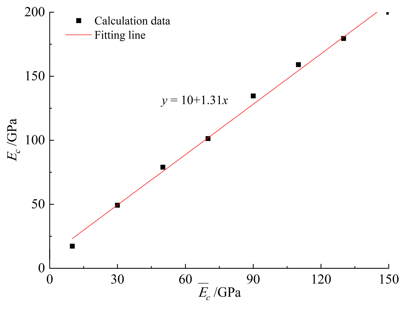
Figure 5.
Relationship between and .
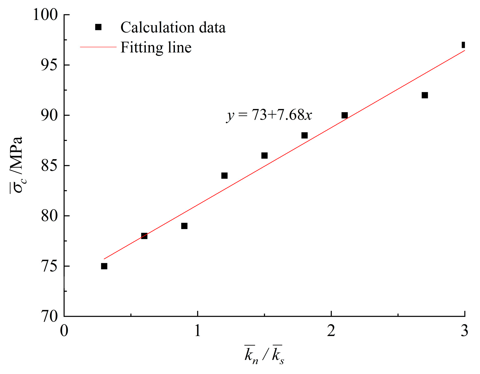
Figure 6.
Numerical calculation model: (a) Uniaxial compression, (b) Brazilian splitting.

Figure 7.
Comparison of numerical calculation and laboratory experiment results: (a) Uniaxial compression, (b) Brazilian splitting.
Figure 7.
Comparison of numerical calculation and laboratory experiment results: (a) Uniaxial compression, (b) Brazilian splitting.


Table 1.
Microparameters of the PBM.
| Parameters of the Particles | Parameters of the Parallel Bonds |
|---|---|
| Modulus of the particles: | Modulus of parallel bonds: |
| Ratio of normal to tangential stiffness of the particles: | Ratio of normal to tangential stiffness of parallel bonds: |
| Friction coefficient of the particles: | Average value of normal strength of parallel bonds: |
| Average value of tangential strength of parallel bonds: | |
| Radius increase factor of parallel bonds: |
Table 2.
Training dataset.
| No. | Input Parameters: (UD Results) | Output Parameters: (Numerical Calculation Results) | ||||||
|---|---|---|---|---|---|---|---|---|
| /GPa | /MPa | /MPa | /GPa | /MPa | /MPa | |||
| 1 | 48.09 | 1.001 | 33.74 | 33.74 | 0.55 | 70.24 | 55.47 | 4.91 |
| 2 | 48.09 | 1.183 | 24.10 | 43.38 | 0.75 | 71.82 | 56.83 | 4.13 |
| 3 | 75.57 | 1.001 | 33.74 | 62.66 | 0.55 | 126.61 | 81.15 | 4.51 |
| 4 | 103.05 | 1.183 | 72.30 | 43.38 | 0.75 | 201.37 | 79.33 | 4.82 |
| 5 | 48.09 | 0.637 | 33.74 | 53.02 | 0.35 | 68.36 | 68.59 | 5.72 |
| 6 | 89.31 | 0.455 | 72.30 | 62.66 | 0.55 | 149.98 | 100.11 | 4.91 |
| 7 | 103.05 | 1.183 | 33.74 | 72.30 | 0.25 | 201.37 | 79.29 | 4.81 |
| 8 | 61.83 | 0.637 | 53.02 | 33.74 | 0.55 | 61.44 | 56.06 | 4.62 |
| 9 | 61.83 | 1.183 | 43.38 | 24.10 | 0.35 | 74.93 | 45.05 | 4.13 |
| 10 | 48.09 | 0.637 | 53.02 | 72.30 | 0.75 | 68.36 | 107.37 | 5.71 |
| 11 | 75.57 | 0.455 | 33.74 | 24.10 | 0.75 | 67.51 | 38.31 | 4.73 |
| 12 | 89.31 | 1.365 | 53.02 | 53.02 | 0.55 | 131.96 | 90.60 | 5.31 |
| 13 | 103.05 | 0.819 | 43.38 | 43.38 | 0.45 | 153.37 | 71.44 | 4.87 |
| 14 | 34.35 | 0.455 | 62.66 | 43.38 | 0.45 | 43.28 | 70.68 | 5.01 |
| 15 | 103.05 | 0.637 | 24.10 | 53.02 | 0.65 | 159.84 | 61.31 | 8.02 |
| 16 | 34.35 | 0.819 | 72.30 | 24.10 | 0.65 | 48.75 | 43.35 | 3.81 |
| 17 | 34.35 | 1.365 | 43.38 | 72.30 | 0.65 | 66.07 | 88.60 | 3.72 |
| 18 | 89.31 | 1.001 | 53.02 | 33.74 | 0.25 | 131.20 | 59.50 | 4.71 |
| 19 | 48.09 | 1.365 | 72.30 | 53.02 | 0.25 | 82.30 | 96.79 | 4.11 |
| 20 | 34.35 | 1.001 | 53.02 | 62.66 | 0.35 | 54.79 | 100.42 | 5.21 |
| 21 | 75.57 | 0.455 | 43.38 | 43.38 | 0.25 | 67.51 | 66.88 | 4.72 |
| 22 | 61.83 | 1.183 | 62.66 | 62.66 | 0.45 | 74.93 | 110.14 | 4.14 |
| 23 | 89.31 | 0.819 | 43.38 | 62.66 | 0.75 | 106.06 | 93.50 | 4.18 |
| 24 | 75.57 | 0.819 | 72.30 | 72.30 | 0.35 | 133.63 | 112.27 | 4.33 |
| 25 | 61.83 | 1.001 | 62.66 | 53.02 | 0.65 | 77.88 | 91.54 | 4.45 |
| 26 | 75.57 | 1.365 | 62.66 | 33.74 | 0.65 | 116.83 | 64.21 | 4.61 |
| 27 | 89.31 | 1.365 | 24.10 | 24.10 | 0.45 | 131.96 | 43.19 | 5.31 |
| 28 | 61.83 | 0.455 | 24.10 | 72.30 | 0.45 | 67.50 | 69.92 | 4.72 |
| 29 | 34.35 | 0.819 | 24.10 | 33.74 | 0.25 | 48.75 | 51.10 | 3.82 |
| 30 | 103.05 | 0.637 | 62.66 | 24.10 | 0.35 | 158.48 | 40.55 | 11.41 |
Table 3.
Macroparameters of marble.
| /GPa | /MPa | /MPa |
|---|---|---|
| 66.1 | 63.9 | 3.8 |
Table 4.
Calibration values of microparameters.
| /GPa | /MPa | /MPa | ||
|---|---|---|---|---|
| 45.72 | 0.94 | 44.83 | 43.37 | 0.497 |
Table 5.
Calculated and experimental values of macroparameters for marble.
| /GPa | /MPa | /MPa | |
|---|---|---|---|
| Experimental values | 66.1 | 63.9 | 3.8 |
| Calculated values | 62.8 | 68.9 | 3.9 |
| Relative error | 5.3% | −7.8% | −2.6% |
Disclaimer/Publisher’s Note: The statements, opinions and data contained in all publications are solely those of the individual author(s) and contributor(s) and not of MDPI and/or the editor(s). MDPI and/or the editor(s) disclaim responsibility for any injury to people or property resulting from any ideas, methods, instructions or products referred to in the content. |
© 2023 by the authors. Licensee MDPI, Basel, Switzerland. This article is an open access article distributed under the terms and conditions of the Creative Commons Attribution (CC BY) license (https://creativecommons.org/licenses/by/4.0/).
Share and Cite
MDPI and ACS Style
Jin, Z.; Chang, W.; Li, Y.; Wang, K.; Fan, D.; Zhao, L. Microparameters Calibration for Discrete Element Method Based on Gaussian Processes Response Surface Methodology. Processes 2023, 11, 2944. https://doi.org/10.3390/pr11102944
AMA Style
Jin Z, Chang W, Li Y, Wang K, Fan D, Zhao L. Microparameters Calibration for Discrete Element Method Based on Gaussian Processes Response Surface Methodology. Processes. 2023; 11(10):2944. https://doi.org/10.3390/pr11102944
Chicago/Turabian StyleJin, Zhihao, Weiche Chang, Yuan Li, Kezhong Wang, Dongjue Fan, and Liang Zhao. 2023. "Microparameters Calibration for Discrete Element Method Based on Gaussian Processes Response Surface Methodology" Processes 11, no. 10: 2944. https://doi.org/10.3390/pr11102944
Note that from the first issue of 2016, this journal uses article numbers instead of page numbers. See further details here.