1. Introduction
The market demand for recombinantly produced biopharmaceuticals has increased rapidly in recent years. Various sources estimate a market cap of 2021 between USD 328 and 407 billion with a projected compound annual growth rate between 7% and 11% [
1,
2,
3,
4]. Monoclonal antibodies alone make up almost half of this market, with market cap estimations between USD 168 and 185 billion [
5,
6,
7]. The rise of monoclonal antibodies (and associated therapeutic proteins, including antibody fragments) can be attributed to their wide-ranging clinical application, as they are used for treatment against (i) cancers, (ii) inflammatory diseases, (iii) neurological disorders, (iv) infections, (v) metabolic diseases, (vi) autoimmune conditions and (vii) cardiovascular diseases [
8,
9,
10]. The rapid growth of the sector resulted in the need for accelerated R&D pipelines. One of the bottlenecks in establishing recombinant protein production processes is the development of the fermentation process, during which genetically modified microorganisms express the protein of interest for subsequent harvesting and purification. In response, high-throughput methodologies in molecular biology have been developed, leading to the generation of sizable libraries of potential recombinant production strains [
11,
12]. The protein of interest produced during fermentation processes conducted in this study is a single-chain variable fragment (scFv), which is an antibody sub-element retaining the antigen binding region of the antibody. These can be produced rapidly and with higher space–time yields than antibodies themselves, and have other potential clinical benefits, explaining the industry’s interest in the production of scFvs [
10].
Screening all potential production strains with traditional lab-scale fermentation systems is time-intensive and associated with high (economic and labor) costs. This gave rise to the need for high-throughput-microbioreactor (HT-MBR) systems capable of simultaneously executing multiple small-scale fermentations under controlled conditions [
13]. As a result, several HT-MBR systems have been developed, commercialized and implemented in both academia and industry [
14,
15,
16,
17,
18]. A fully automated MBR system based on four temperature controlled bioREACTOR 8 (2mag AG, Munich, Germany) fermentation blocks has been developed and implemented at the Boehringer Ingelheim Regional Center, Vienna; this has previously been described elsewhere [
19,
20]. We return to the operation of this system in more detail in our methodology section (
Section 2).
One concern with MBRs is that frequent sampling of the fermentation broth causes large percentage volume changes in comparison to large-scale fermenters [
21]. These volume changes may have repercussions on the overall fermentation performance and therefore also on the meaningfulness and scalability of MBR experiments. Moreover, sampling occupies liquid-handling (LiHa) robotic pipetting arms, which are responsible for the supplementation of essential process fluids, such as the carbon feed, as well as acid and base additions. These operations cannot be performed during sampling. Whilst pH fluctuations are negligible, as acidification of the fermentation broth occurs at a slow pace at the relatively low cell densities encountered in MBR systems, intermittent carbon source limitations that occur during sampling represent a greater problem for the microorganism’s metabolic state. Therefore, it is desirable to minimize the number of samples taken for at-line and offline measurements in MBR systems.
Soft sensors present a solution to the above-described challenge. These are model-based systems designed to estimate relevant process variables in real time where physical sensors cannot provide accurate online monitoring due to technical limitations. Soft sensors can be subdivided in three categories: (a) mechanistic models [
22], (b) statistical models [
23,
24] and (c) hybrid models [
25,
26,
27]. Below, we outline the differences between these categories and explain our choice of the statistical model.
Mechanistic models, (a), are based on one or more equations derived from first principles that describe direct coherence between accessible process variables and estimated key process variables [
28,
29]. The development of mechanistic models requires in-depth knowledge of the relevant process and moderate understanding of supporting process variables. Another approach to soft sensors, (b), is data-driven statistical modelling. These models are fitted to historical data from previous experiments, which represent the past behavior of the process. Statistical tools such as decision trees [
30], multiple linear regression [
31] or artificial neural networks (ANNs) [
32] can be applied to develop the underlying models for soft sensors of this type. In comparison to mechanistic models, statistical models can detect more complex process behaviors due to their adaptive nature and require fewer supporting process variables. However, they require a sizable amount of historical experimental data as well as in-depth knowledge on the development and evaluation of statistical models.
Hybrid models, (c), are a combination of mechanistic and statistical models. One common approach to hybrid models is the development of sequential models where mechanistic models make initial estimations of intermediate process variables; these variables are subsequently used as inputs for statistical models. Alternatively, the statistical model may be used to produce intermediate estimates which can then be used in the mechanistic model [
33,
34,
35]. Parallel hybrid models consist of mechanistic and statistical models running in parallel, with the joint output being the final estimation [
36]. Mechanistic and hybrid models have been used for the estimation of biomass during fermentation in previous studies [
37,
38,
39]. However, these models relied on data generated through substrate quantification or off-gas analysis, which (to date) is not available in most MBR systems. The strength of MBR systems lies in the rapid generation of large quantities of experimental data, which balances out one of the main drawbacks of statistical models: the requirement of large datasets for model generation and evaluation. Therefore, statistical models are an attractive choice for modelling bioprocesses in MBR systems.
One of the most powerful statistical models are ANN models, on which our soft sensor is based (see
Section 2). Interest in the field of ANNs surged in recent years; this can be attributed to the availability of vast quantities of data, increased computational power and improved training algorithms [
40,
41]. It has been shown multiple times that ANNs represent one of the most powerful machine learning methods available, with applications ranging from comparatively simple tasks such as speech [
42] and image recognition [
43] to more complex tasks such as autonomous driving [
44] as well as creative tasks such as music composition [
45]. We return to their operation in more detail in our methodology section (
Section 2); however, the basic principle behind ANNs is that a function is estimated which links a set of specified inputs to a desired output by minimizing the functions´ error via gradient descent optimization. Each training iteration during gradient descent consists of an initial estimation of the target values and a subsequent update of the models´ weights along the gradient of the error with respect to the weights [
46].
The greatest challenge regarding the development of an OD soft sensor for high-throughput MBR systems is that only a limited set of meaningful process parameters (such as the base addition, carbon feed and inducer addition, as well as pH, temperature and dissolved oxygen (DO)) is available as online parameters. Further, only a few of these parameters are directly linked to the OD. The OD soft sensors presented in our study are based on ANN models, these models having been successfully used to generate models describing bioprocesses. For example, Zhu et al. (1996) used an ANN to predict lysine production during a
Brevibacterium flavum fermentation based on sugar consumption, accumulated CO
2 and the respiratory quotient [
47]. Murugan and Natarajan developed an ANN-based soft sensor that predicted the biomass based on pH, agitation speed, substrate concentration and earlier biomass measurements [
48]. However, the ANNs used in these aforementioned studies used variables that require offline measurements for prediction. Hence these models could not be used for fully automated real-time monitoring.
In contrast, Melcher et al. and Zhu et al. (2020) trained ANNs based purely on online measurements [
49,
50]. These were designed for larger-scale processes where informative variables stemming from, e.g., off-gas analysis or fluorescence spectroscopy, were available. One of the challenges in this study, by comparison, was that these measurements were not available for modelling. The overall aim of this study was therefore to develop an ANN-based soft sensor for the real-time estimation of cell density in a high-throughput MBR system. Studies describing the development of such soft sensors have not been published to date.
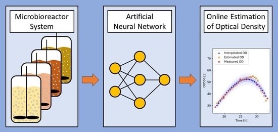
Implementation of the presented OD soft sensor is expected to increase the overall scalability and predictive power of fermentation conducted with MBR systems, by enabling a reduction in physical OD measurements without significant information loss. Additionally, the OD soft sensor will improve online monitoring and enable OD-dependent process control. We propose that the presented OD soft sensor can be applied to similar MBR systems and provide significant benefits, particularly for MBR systems not capable of glucose quantification or off-gas analysis.
2. Materials and Methods
2.1. High-Throughput-Microbioreactor System
The operating procedures of the MBR system developed and implemented at the Boehringer Ingelheim Regional Center, Vienna will be discussed briefly in this article; however, a detailed description can be found elsewhere [
19]. The centerpiece of the MBR system is a set of four fermentation blocks (bioREACTOR8; 2mag AG; Munich, Germany), each holding eight sterile single-use MBRs (Mini-Bioreactors HTBD LG1-PSt3 Hg; PreSens GmbH, Regensburg, Germany) equipped with fluorometric sensor spots for online pH and dissolved oxygen (DO) measurements, which are placed under a HEPA filter (BDK Luft- und Reinraumtechnik, Sonnenbühl, Germany) to ensure sterile operation. The 32 single-use 15 mL bioreactors are equipped with fluorometric sensor spots for measuring DO and pH [
20]. The stirred MBRs are supplemented with essential fluids such as base, acid and carbon source by a liquid-handling (LiHa) arm via a Tecan Freedom EVO 200 robotics system (Tecan Group, Männerdorf, Switzerland). This robotics system is also responsible for transporting microplates and deep-well plates between peripheral elements of the MBR setup. Fully automated OD measurements for biomass quantification are performed at-line by a microplate spectrophotometer (SPECTRAmax PLUS384; Molecular Devices Corporation, San Jose, CA, USA). To measure the OD, samples are taken by the LiHa robotic arm and subsequently 1:10, 1:50 and 1:200 dilutions are performed within a 96-well microplate, which is then transported to a spectrophotometer (SPECTRAmax PLUS384; Molecular Devices Corporation, San Jose, CA, USA) for the final OD quantification at a wavelength of 550 nm. The relative standard deviation of the OD measurement was determined to be 4.7% throughout the operating range. Samples taken for offline analysis, mostly for titer quantification, are stored in a deep freezer at −20 °C (STR44-DF; Liconic Instruments, Montabaur, Germany). The temperature of the MBRs is regulated with a temperature-controlled water circuit that flows through the fermentation blocks. The DO within the MBRs is regulated with a cascade controller, first varying the agitation rate from 1900 to 2800 RPM followed by oxygen supplementation to a maximum of 50%
v/
v.
2.2. Data Generation
To generate the diverse dataset required for the development of the ANN-based OD soft senor, a design of experiments (DoE) case study with four different scFv-expressing Escherichia coli (E. coli) BL21(DE3) strains was conducted. This allowed us to train and validate the OD soft sensor on fermentations executed under varying process conditions.
The expression systems of strains 1–3 were genome-integrated, while the expression system of strain 4 was plasmid-based. All strains contained the same IPTG inducible scFv expression system, controlled by a T7 promotor and a lacI regulator. Additionally, strains 1 and 2 expressed different combinations of helper factors. The plasmids that encoded the helper factor genes of strains 1 and 2 were induced with a second inducer (inducer 2; compound name confidential).
A two-level, five-factor irregular-fraction design with 32 experiments and eight center points was used for the initial parameter screening of strains 1 and 2. For strains 3 and 4, a two-level four-factor factorial design, also with 32 experiments and eight center-points was used. The varied process parameters were temperature, pH, induction length, IPTG concentration and in the case of strains 1 and 2, the inducer 2 concentration. The temperature was varied in a range of 12 °C, the pH in a range of 1.2, the IPTG concentration in a range of 400 µM and the induction length in a range of six hours. Design plans were augmented for subsequent parameter optimization, which included duplicate face-centered design points and six center points resulting in an additional 26 experiments for strains 1 and 2 and 22 experiments for strains 3 and 4. The generation of the design plans was performed with DesignExpert 11 (Stat-Ease, Minneapolis, MN, USA).
All processes were conducted with chemically defined batch and feed medium. Once the carbon source within the batch medium was exhausted, a feeding scheme was initiated that consisted of a two hour long exponential feed phase, followed by a linear feed that lasted until the end of the process. Four hours into the feed phase, the inducers were added to the fermentation broth to initiate scFv and helper-factor production.
2.3. Data Processing and Model Development
An overview of the data processing and model development pipeline is given in the form of a flowchart in
Figure 1. The data generated with the MBR system was stored in a data warehouse and retrieved using InCyght software (Exputec, Vienna, Austria). The data was then exported to Microsoft Excel (Microsoft, Redmond, WA, USA) and finally imported to Python 3.7.5. (Python Software Foundation, Wilmington, NC, USA) where all further data engineering and handling was performed. Numeric operations were performed using Numpy 1.20.3 and pandas 1.1.2 [
51,
52]. All plots were generated with matplotlib 3.3.1 [
53].
Interpolation was carried out for all parameters (pH, DO, temperature, addition of base/acid, addition of carbon feed, addition of inducer, process volume, agitation rate, oxygen flow and OD) to align the measurement frequency of the entire data set (e.g., pH measurements were every five seconds, while OD measurements were hours apart). For all liquid additions and the process volume, the last available value was propagated forward until the next change of value. The pH, DO, temperature, agitation rate and oxygen flow were interpolated linearly. Third order smoothing splines from SciPy 1.6.2 (scipy.interpolate.UnivariateSpline) were chosen for the OD as individual measurements were hours apart, and the resulting data followed a curvilinear relationship that cannot be described accurately with linear interpolation [
52,
54,
55]. The interpolated OD was taken as the best estimate of the OD without additional physical measurements. Smoothing splines mitigate the influence of measurement noise—with the exception of infeasible outliers—on the spline fit as they are not forced exactly through the datapoints. Nevertheless, the quality of the OD interpolation was evaluated by plotting the interpolated data together with the measured data, which was followed by an analysis for feasibility. OD outliers were first identified by utilizing boxplots to compare individual growth rates to the corresponding growth rate populations observed during fermentations of the same strain and removed in case of unfeasibility. Fermentations where the first or last OD measurements, or more than two others, were considered unfeasible, were not used for modelling.
A set of up to 65 inputs was extracted from the process data for each 30 min period post-induction to train the ANN models and estimate the OD during testing. The main inputs utilized for estimation were the volume-specific cumulative ammonia and volume-specific carbon feed additions at the time of estimation. As it was assumed that the past behavior of the volume-specific cumulative ammonia addition contains valuable information, its value at the end of each 30 min interval of the ten hours prior to each estimation point was used for modelling. Further, the volume-specific cumulative ammonia addition rates at each of those timepoints were calculated and converted to inputs. Another input subset consisted of DO-dependent parameters, such as the cumulative time, for which the DO was at 0%.
Cross-validation is an essential step in the development of ANN models as it reduces overfitting, increases the model´s generalization capability, and ensures that the model is capable of correctly estimating target values for unseen data. Therefore, inputs were subdivided fermentation-wise into three different data sets of varying sizes:
- (a)
The training set contained 70% of all available fermentations and was used to fit the ANN models;
- (b)
The validation set contained 15% of all available fermentations and was used to detect overfitting, in which case model training was stopped;
- (c)
The test set contained 15% of all available fermentations and was used for model validation.
To ensure an even distribution of fermentations of similar OD characteristics, each fermentation was first allocated into one of four groups based on the volume-specific cumulative base addition (<0.06 µL ammonia/µL process volume, 0.06–0.07 µL/µL, 0.07–0.075 µL/µL and >0.075 µL/µL) at the end of the process. The data was subsequently split from the four groups into each of the three aforementioned subsets. The OD itself was not used as a splitting criterion, as it is not a given that two processes with the same OD at the end of each process had similar ODs throughout the process. In total, ten random data splits were performed. To ensure that all model inputs were in the range between 0 and 1, min/max normalization was applied.
To simulate the validation and test data being unknown, the maximum and minimum values of each variable (x) were taken from training set data.
2.4. Artificial Neural Networks
All models investigated in this study are feed-forward ANNs. ANNs are machine learning models that learn to estimate response
y from input data
X. They consist of multiple hidden layers each containing a set of neurons. Each neuron computes a linear combination
z of
n inputs
xi, their corresponding weights
wi and a bias
b.
For the ANN to be able to learn non-linear correlations, a non-linear activation function is used to transform
z. In this study the leaky ReLU activation was used; however, other activation functions such as sigmoid or hyperbolic tangent are also in common use. Leaky ReLU is a linear function with an angle at the origin [
56]. The degree of the angle is defined by parameter
α, where smaller values of
α result in a more pronounced non-linearity. The leaky ReLU function is shown in Equation (3).
The transformed output of each neuron is then forwarded to the next hidden layer. ANNs are trained by updating the model weights to reduce the model loss
L. This is achieved via gradient descent, where the weights are changed in the opposite direction of the gradient of the weights with respect to
L scaled by the learning rate
λ.
The most common losses used for regression problems are the mean squared error (MSE) and the root mean squared error (RMSE), the latter of which is defined by Equation (5), where
is the ANN prediction.
To prevent the ANN from overfitting,
L is repeatedly evaluated on the validation set. An increasing validation loss is an indicator of overfitting, at which point training is stopped. This process is commonly referred to as early stopping. It is common practice to initialize ANN weights randomly at the beginning of training. Various strategies for initializing the weights have emerged over the years [
57]. Most initializers sample from either a normal or uniform distribution. The initializer used in this study samples from a normal distribution for each layer with mean zero and a variance of
where
is the number of each layer´s inputs.
All ANN models were generated using Google’s Tensorflow 2.5.0. (Google, Mountain View, CA, USA) Python library [
58]. The model hyperparameters were optimized using a Python script that compared the accuracies of models trained with multiple hyperparameter combinations. This process is represented by the loop in
Figure 1, and a more detailed description of the algorithm can be found in
Appendix A. An overview of the final hyperparameters is presented in
Table 1. For model selection, 100 models were trained using the optimized set of hyperparameters. The model that resulted in the smallest MSE for the validation set and the smallest sum of the MSEs for the training and validation sets was picked for further analysis.
3. Results
3.1. Overview of the Data
For the generation of robust probabilistic models, it is essential that a broad feature space of both the estimated variable as well as the covariates is encapsulated within the dataset. Therefore, a five-factor DoE study was performed with variations in temperature, pH, induction length and the inducer concentration of two different inducers. In the following, we present an overview of the data this study yielded, and our analysis of these data.
The interpolated OD time-series data of all experiments used for model generation are visualized in
Figure A1. Strains 1 and 3 had the most similar growth characteristics with the bacteria entering a stationary phase or decline phase between 27 and 30 h of process time in most experiments. In the case of strain 2, the biomass generally increased linearly until the end of the bioprocess. In contrast, strain 4 generally did not grow as well as the other strains, as the beginning of the decline phase was frequently reached between 22 and 25 h of process time. The different growth characteristic of strain 4 can be attributed to the plasmid-based expression system. The batch phase in experiments of strain 4 was also usually approximately two hours shorter than that of the other strains.
Fundamental descriptive statistics of the final OD values for each strain are summarized in
Table 2. Comparing the mean, standard deviation, 75% and 25% quartiles, and maximum and minimum of the distributions of the final OD of strains 1 and 3 further underlines their similarity. The overall observed maximum of the final OD was 79.1 and the minimum was 21.3, which shows that the different process conditions combined with the use of different strains resulted in different growth behaviors. Therefore, an OD soft sensor that can estimate the OD for this dataset accurately can be considered robust due to the broad feature space encountered in this dataset.
To gain insight into the biologically and methodologically induced variation of the OD, center-point experiments of the DoE study—which had identical process parameter set points—were analyzed and compared with one other. Additionally, the variation of the cumulative base addition was investigated in comparison with the variation of the OD. Similarities between these quantities would indicate that the variation of the OD was not an artefact due to measurement errors, but that individual experiments resulted in different growth behaviors. Furthermore, the cumulative base addition was of particular interest, as this covariate has previously been shown to be strongly correlated to the biomass, and variations of the cumulative base addition between runs might therefore explain observed differences in the measured OD.
As the measured OD at induction was used as a model input and designed to predict the OD exclusively during the induction phase, only the variation of the OD and cumulative base addition during the induction phase were of interest. To analyze these variations, initial measurements were aligned at the origin in order to remove variation developing pre-induction. For this purpose, the OD value and time at the first measurement was subtracted from all data points of the respective experiment. The cumulative base addition was likewise aligned to the initial OD measurement. The aligned data are visualized in
Figure 2 and the standard deviations of the OD and the cumulative base additions at the time of the measurements are summarized in
Table 3. The standard deviations of both the OD and the cumulative base addition generally increased over time, with the exception of the standard deviation of the OD of strain 2. The standard deviations for all strains fall within the expected range; differences can be explained by measurement inaccuracies, biological variation and process variation stemming from the HT-MBR system.
3.2. OD Soft Sensor Performance
Initially, four ANN models were trained: one model for each of the four strains, and one single ANN model trained on the entire dataset. Some expected advantages of a multi-strain model include: (a) significant reduction in the development time for model generation; (b) reduction in complexity of the final soft sensor, avoiding the requirement to switch between strain-specific models; (c) expansion of the variable space of the models; and (d) greater ease in capturing strain independent growth characteristics, given the availability of more training data.
The average normalized RMSE-based accuracy of the strain-specific ANN models on the respective test sets was 94.34%. A more detailed performance summary of the strain-specific models can be found in
Table A1. Before the single model for all strains was trained, strain identification parameters were added to the data inputs using one-hot encoding. This modification, allowing the model to distinguish between the different strains, was beneficial in improving model accuracy given the different growth characteristics of the strains. The combined model resulted in an accuracy of 95.14%, surpassing the previous benchmark of the four individual models. The standard deviation of the OD measurement of 4.7% placed a limit on maximal achievable accuracy; further model improvements were therefore not readily attainable beyond this point. It could be reasonably expected that the performance gain of combined models compared to individual models would be more pronounced for smaller datasets.
Additional performance indicators of the combined OD soft sensor are presented in
Table 4. The spread in the RMSE between the training and test sets was minor, and therefore overfitting was not considered to be an issue. Additionally, the percentage of estimations within the tolerance interval of the measured OD values of one standard deviation (σ) and two standard deviations (2σ) were calculated to gain insight into the distribution of the prediction errors. The accuracy achieved by the combined model can be viewed as an excellent result.
3.3. Generalized OD Soft Sensor
While the models described earlier are capable of estimating the OD of different strains accurately, they rely on training data of all four strains as well as on strain identification markers. Therefore, the model is not capable of estimating the OD for unknown strains during de novo fermentations. To remedy this shortcoming, a generalized OD soft sensor was developed that can estimate the OD during de novo fermentations.
To generate the generalized OD soft sensor, the strain identification markers were removed and ANN models were trained on data only of specific strains. The resulting models were then tested using external test sets, which included fermentation data generated during processes of the other remaining strains, which means that the models had to estimate the OD for fermentations of previously unseen strains. In total, three models were generated and tested in this way. The first model, which will be referred to as model 2, was trained on data of strain 2 and tested using data of strains 1, 3 and 4. Model 24 was trained on data of strains 2 and 4, and tested on data of strains 1 and 3, and model 124 was trained on data of strains 1, 2 and 4, and tested on data of strain 3. The data from fermentations of strain 2 was included in all models as strain 2 behaved in the most predictable manner as decline phases rarely occurred. Fermentations with strain 2 resulted in the highest final OD values. For model 24, data from fermentations of strain 4 was also added, as strain 4 showed the most non-linear behavior and resulted in the lowest final OD values. Therefore, the whole variable space was mostly covered with these two strains. Finally, to train model 124, data of fermentations of strain 1 were added. The performance indicators of all three models are presented in
Table 5. The accuracy for the external test set increased with the number of strains that were used for training.
All three models achieved both an overall accuracy and an accuracy for the test set of above 94% for the strains they were trained on. The accuracy for the external test set was unsatisfactorily low with 84.32% for the simplest model; however, the accuracy increased substantially with additional training data of the other strains, reaching an accuracy of 91.37% for the external test set of model 124. The progression of the model estimation capabilities, based on two example experiments of strain 3 with different growth profiles, is shown in
Figure 3.
In the first example shown in
Figure 3A–C, model 2 incorrectly estimated an OD increase throughout the process. This was most likely due to the rare increases in OD in the training set of model 2. In contrast, model 24 identified the OD decrease and model 124 replicated the OD accurately. Similarly, in the second example illustrated in
Figure 3D–F, model 2 underestimated the OD throughout the process, whilst the expansion of the training set for model 24 as well as model 124 refined the model estimations further.
The evidence presented in
Table 5 and
Figure 3 suggests that the OD soft sensor is capable of estimating the OD for unknown strains of appropriate similarity with acceptable accuracy. One can only expect a similar generalization performance when the variable space is covered by the training data and the models perform well on the strains in the training data. Therefore, the model is not expected to yield accurate results for highly dissimilar fermentation processes, such as yeast fermentations. However, it can be assumed that the estimation quality for unknown strains will continue to increase with the number of different strains included within the training set. As the database of processes increases over time, retraining will lead to more accurate models, which have improved generalization capabilities.
3.4. Information Retention for Processes with Fewer Measurements
In order to evaluate the soft sensor under post-implementation conditions, where fewer OD measurements will be taken, eight fermentation runs were performed for all four strains. Process parameter set points were identical to the ones used for the center point experiments of the DoE study, and only three OD measurements were taken. The data were subsequently used to evaluate the OD soft sensor, which resulted in a RMSE of 3.88 and a NRMSE-based accuracy of 92.27%. 45.20% of estimations were within σ and 74.60% were within 2σ.
Upon initial examination, the estimation performance may appear worse when compared to the estimation performance for fermentations with five OD measurements. However, the performance evaluation was assessed using OD values derived from spline interpolation. As fewer OD measurements were taken, the spline interpolations have most likely underfitted the true OD, since peaks that occurred between measurements, were not captured correctly. This behavior was most pronounced for strain 3, where a peak that typically occurred at 30 h was missed when applying the measurement regime with only three measurements, which can clearly be seen in
Figure 4.
In order to determine whether or not the soft sensor could identify these missed peaks, the three measured OD values obtained from experiments with the sparse measurement regime, the corresponding OD soft sensor estimates and the average OD of each measurement performed during the respective experiments with five OD measurements, were compared (
Figure 5). When analyzing the soft sensor estimates for strain 3 (
Figure 5C), it can be seen that the soft sensor estimated the peak that was typically observed at 30 h during fermentations with five OD measurements correctly. A similar yet less pronounced behavior was observed for strain 1 (
Figure 5A). The model underestimated the OD for fermentations with strain 2 (
Figure 5B). The soft sensor was capable of estimating challenging, highly non-linear fermentations with strain 4, where the OD dropped significantly (
Figure 5D). It should also be noted that the interpolated OD may not have described the true OD correctly, aside from the missed peak, as the quality of the spline interpolation probably suffered due to the reduction in available data points.
In summary, the examples presented indicate that the soft sensor could correctly estimate the OD of four different scFv-expressing E. coli strains with different growth characteristics ranging from linear to moderately and highly non-linear growth. As the OD soft sensor was capable of achieving accuracies of over 92% (which is assumed to be an underestimation of the true accuracy due to underfitting of the interpolated OD) it can be concluded that the presented OD soft sensor provides a viable alternative to the previously employed measurement scheme with five OD measurements.
4. Discussion
This study has demonstrated the utility of ANNs in the development of a soft sensor to estimate the OD during E. coli fermentations conducted in a high-throughput MBR system with strains of varying growth characteristics in real time. A generalized OD soft sensor was developed that was able to estimate the OD of unknown strains with an accuracy of >91%, and scaled with the number of strains within the training set. For this reason, we expect the estimation quality to increase with the growth of databases. Finally, the OD soft sensor was tested on fermentations during which a reduced number of physical OD measurements were executed. An accuracy of over 92% was achieved, which was comparable to the 95% achieved on the initial test data. However, as OD peaks were missed during experiments taking only three measurements; the interpolated OD failed to accurately represent the true OD, resulting in an underestimation of the soft sensor accuracy.
Implementation of the presented OD soft sensor would enable model-based predictive control and allow for a reduction in OD measurements. This can be reasonably expected to improve the overall meaningfulness and scalability of data generated with MBR systems. It must be mentioned that the model should be validated repeatedly post-implementation to ensure that potential distributional shifts within the data do not affect its performance. In the case that performance does suffer, the model must be retrained. In a similar spirit, the model should also be retrained when data from other cellular hosts expressing different products are generated, to expand its capabilities continuously. Over time the model will then also learn to predict the OD under these process conditions. Therefore, we want to emphasize the importance of proper data management, which is essential for time-efficient model retraining. Additionally, there is clear ground for future research to adapt the OD soft sensor to estimate other performance variables (e.g., product titer) and test this on different MBR systems.
Although the models already performed well in various settings, it is theoretically possible that further attempts to improve performance might arise from more rigorous input variable selection. It would also be interesting to investigate whether expanding the model to include a mechanistic part could further improve its performance. This, however, poses a significant challenge, as hybrid models require the construction of material balances that usually rely on off-gas analysis, which is not performed in the current iteration of the HT-MBR system used in this study. Another approach to improving the model could be to use ensembles of multiple different machine learning models. It must be kept in mind, however, that this would also increase the resources required for retraining the model. One might also consider improving the explainability of the model by applying methodologies such as the permutation feature importance, Shapley Additive exPlanations or partial dependence plots [
61,
62,
63,
64].


