Article

Averaging Level Control to Reduce Off-Spec Material in a Continuous Pharmaceutical Pilot Plant

Department of Chemical Engineering, Massachusetts Institute of Technology, 77 Massachusetts Avenue, Cambridge, MA 02139, USA
*
Author to whom correspondence should be addressed.
Current address: Department of Process & Energy, Delft University of Technology, Delft 2628, The Netherlands.
Current address: Department of Chemical Engineering, Loughborough University, Loughborough LE11 3TU, UK.
Processes 2013, 1(3), 330-348; https://doi.org/10.3390/pr1030330
Submission received: 13 September 2013 / Revised: 26 October 2013 / Accepted: 25 November 2013 / Published: 29 November 2013
(This article belongs to the Special Issue Feature Papers)

Abstract

:
The judicious use of buffering capacity is important in the development of future continuous pharmaceutical manufacturing processes. The potential benefits are investigated of using optimal-averaging level control for tanks that have buffering capacity for a section of a continuous pharmaceutical pilot plant involving two crystallizers, a combined filtration and washing stage and a buffer tank. A closed-loop dynamic model is utilized to represent the experimental operation, with the relevant model parameters and initial conditions estimated from experimental data that contained a significant disturbance and a change in setpoint of a concentration control loop. The performance of conventional proportional-integral (PI) level controllers is compared with optimal-averaging level controllers. The aim is to reduce the production of off-spec material in a tubular reactor by minimizing the variations in the outlet flow rate of its upstream buffer tank. The results show a distinct difference in behavior, with the optimal-averaging level controllers strongly outperforming the PI controllers. In general, the results stress the importance of dynamic process modeling for the design of future continuous pharmaceutical processes.

Graphical Abstract

1. Introduction

Continuous manufacturing holds promise to improve the reliability and profitability of future pharmaceutical processes [1,2,3,4,5,6]. Significant progress has been achieved to exploit continuous operation of various unit operations that are typically used in pharmaceutical processes [7,8,9,10,11,12,13,14,15,16,17,18,19,20,21,22,23,24,25,26,27,28,29,30,31,32,33,34]. Furthermore, system-wide benefits may exist by, for example, exploiting material recycling and improved process control based on real-time understanding of the final product quality, as well as critical material attributes of streams within the process. Consequently, pharmaceutical companies are interested in the potential benefits of transforming the manufacturing of pharmaceutical products from a conventional batch-wise mode of operation to continuous flow mode [35]. The role of process modeling is expected to increase significantly during this transition to enable improved design and operation [33,36,37,38,39,40,41,42,43].
A key ingredient in enabling the reliable operation of continuous pharmaceutical manufacturing processes is the development of automated control strategies. In particular, judicious use of the buffering capacity of tanks is needed to avoid high concentrations of impurities in a small fraction of the produced tablets and to avoid sharp variations in flow rate propagating throughout the complete process. However, on the downside, extensive use of buffering capacity will lead to sluggish process behavior. Therefore, an appropriate design of automated control strategies around buffer tanks is of importance for the viability of continuous pharmaceutical manufacturing.
The aim of this paper is to identify the potential benefits of using optimal-averaging level control [44] over conventional proportional-integral (PI) feedback level control for an integrated continuous pharmaceutical pilot plant. The pilot plant was constructed within the Novartis-MIT Center for Continuous Manufacturing to produce a pharmaceutical product from start (raw materials for intermediate compounds) to finish (tablets in final dosage form) in a fully continuous fashion [45] and features several cascades of well-mixed tanks. The level of all tanks within the pilot plant were initially controlled with proportional (P)-feedback control only. A plant-wide dynamic model is used to investigate the potential benefits of replacing these level control loops with more advanced control strategies. The plant-wide dynamic model is presented in detail elsewhere [42] and has been extended with control loops in subsequent work [43].
The focus of this paper is on a characteristic sequence of unit operations within the continuous pharmaceutical pilot plant. A closed-loop model is used to simulate the behavior of the unit operations, including automated control loops with P-feedback control. The unknown parameters and initial conditions are estimated from experimental data, which includes the behavior of several level control loops and a concentration control loop in the presence of a significant disturbance and a setpoint change. The focus is on the main compounds in the system to obtain a realistic description of at least the overall mass balance, such that control strategies for buffering can be investigated. Subsequently, the closed-loop dynamic model is used to investigate the potential benefits of replacing the P-feedback level controllers with more extended controllers. First, we will focus on PI level controllers with tuning rules that specifically aim to achieve averaging level control (PI-ALC). Second, process simulations are investigated, where the conventional level controllers are replaced with optimal averaging level control (OALC). The advantage of OALC over conventional PI-ALC is that with OALC, flow optimality can be achieved for a known magnitude of an input disturbance. The results illustrate the importance of advanced control strategies to exploit systematically the buffering capacity of a cascade of buffer tanks in future continuous pharmaceutical processes.

2. Approach

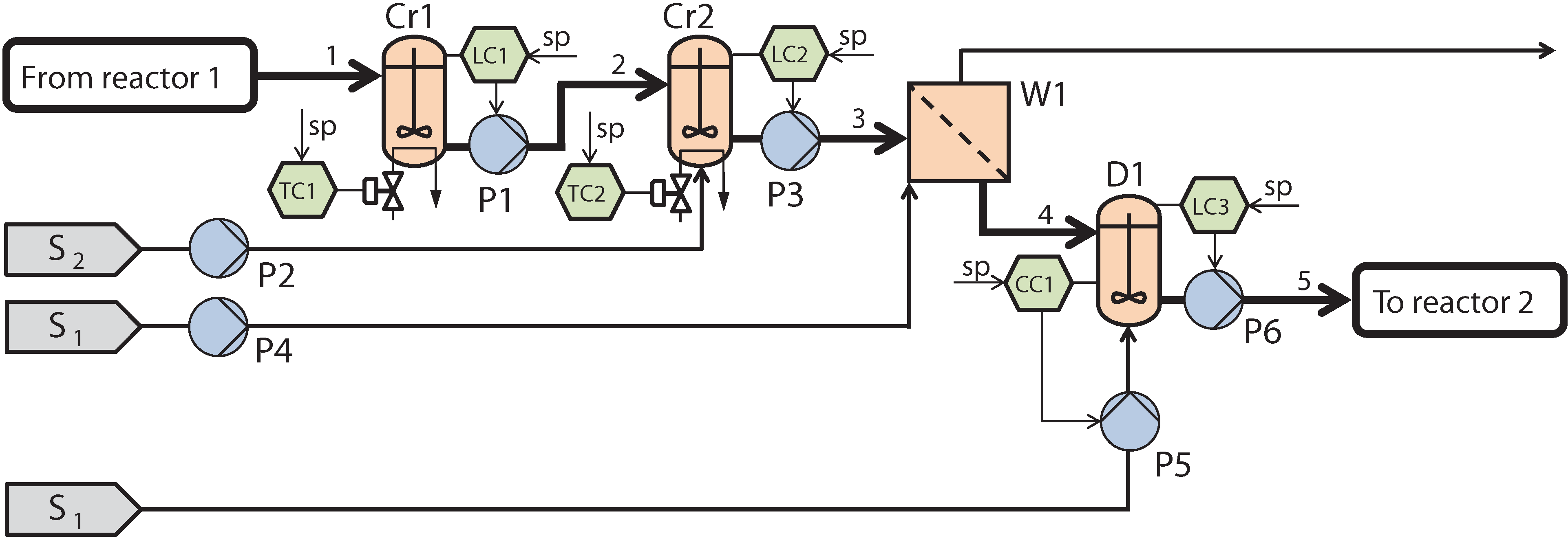
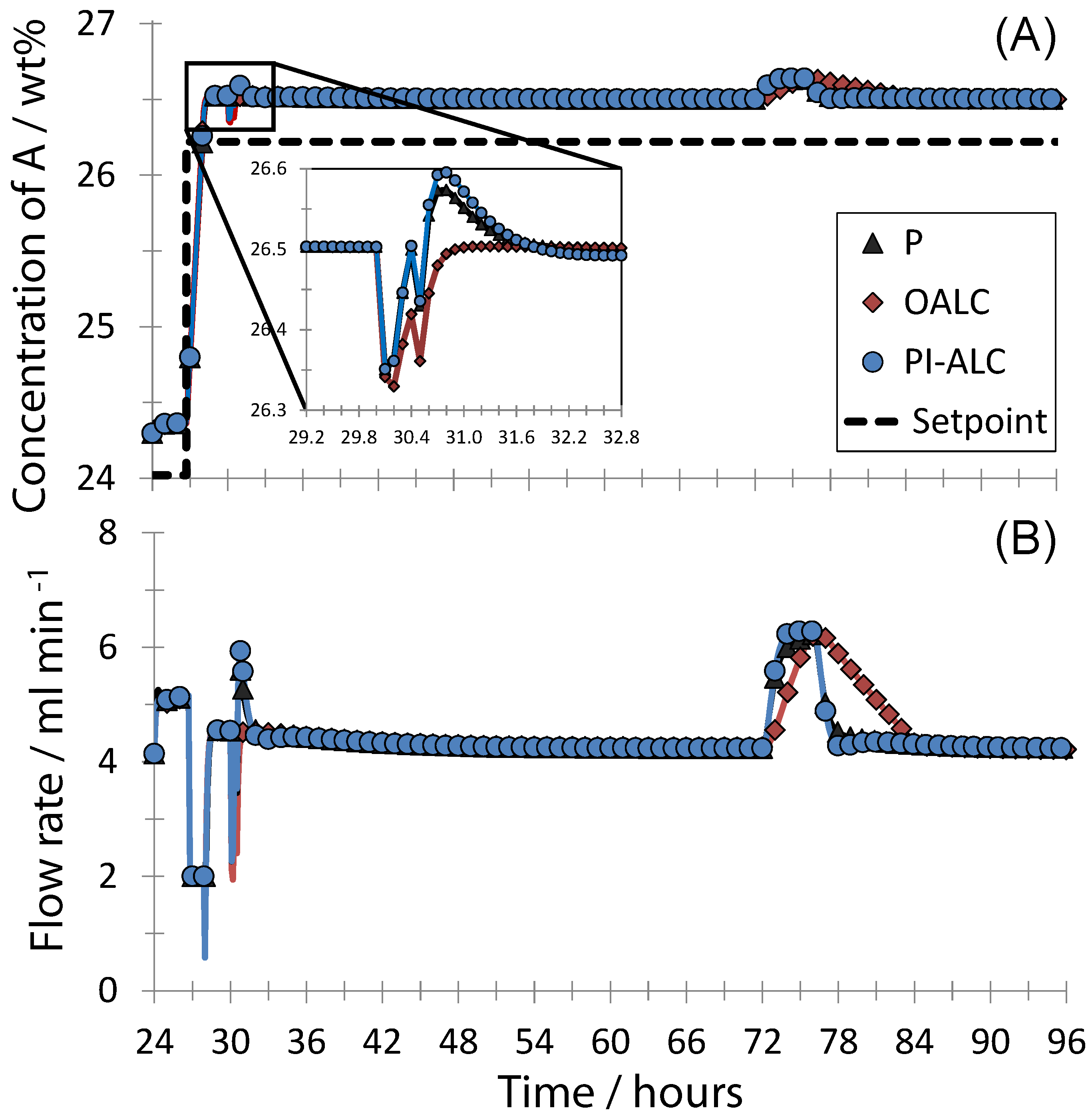
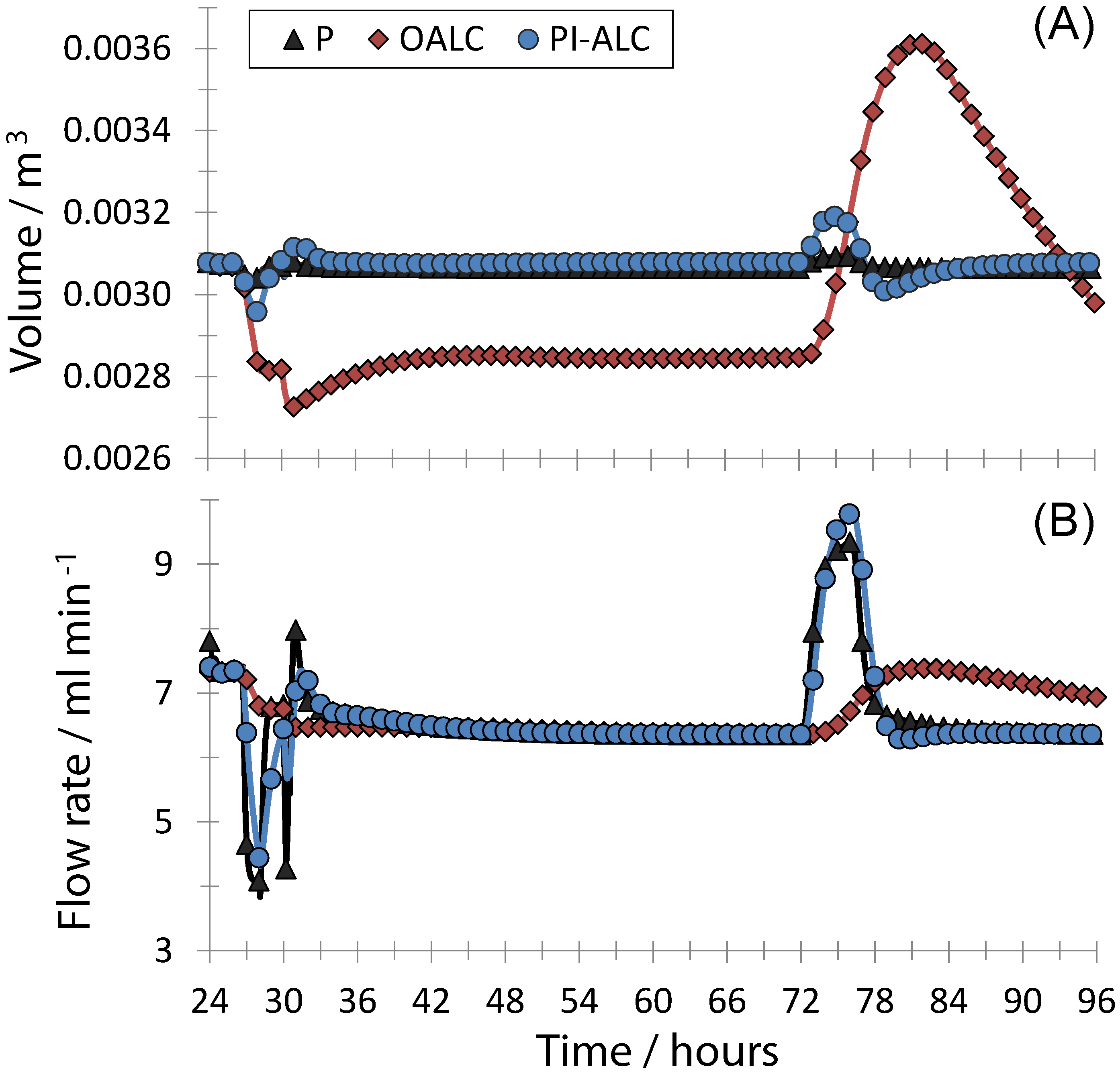
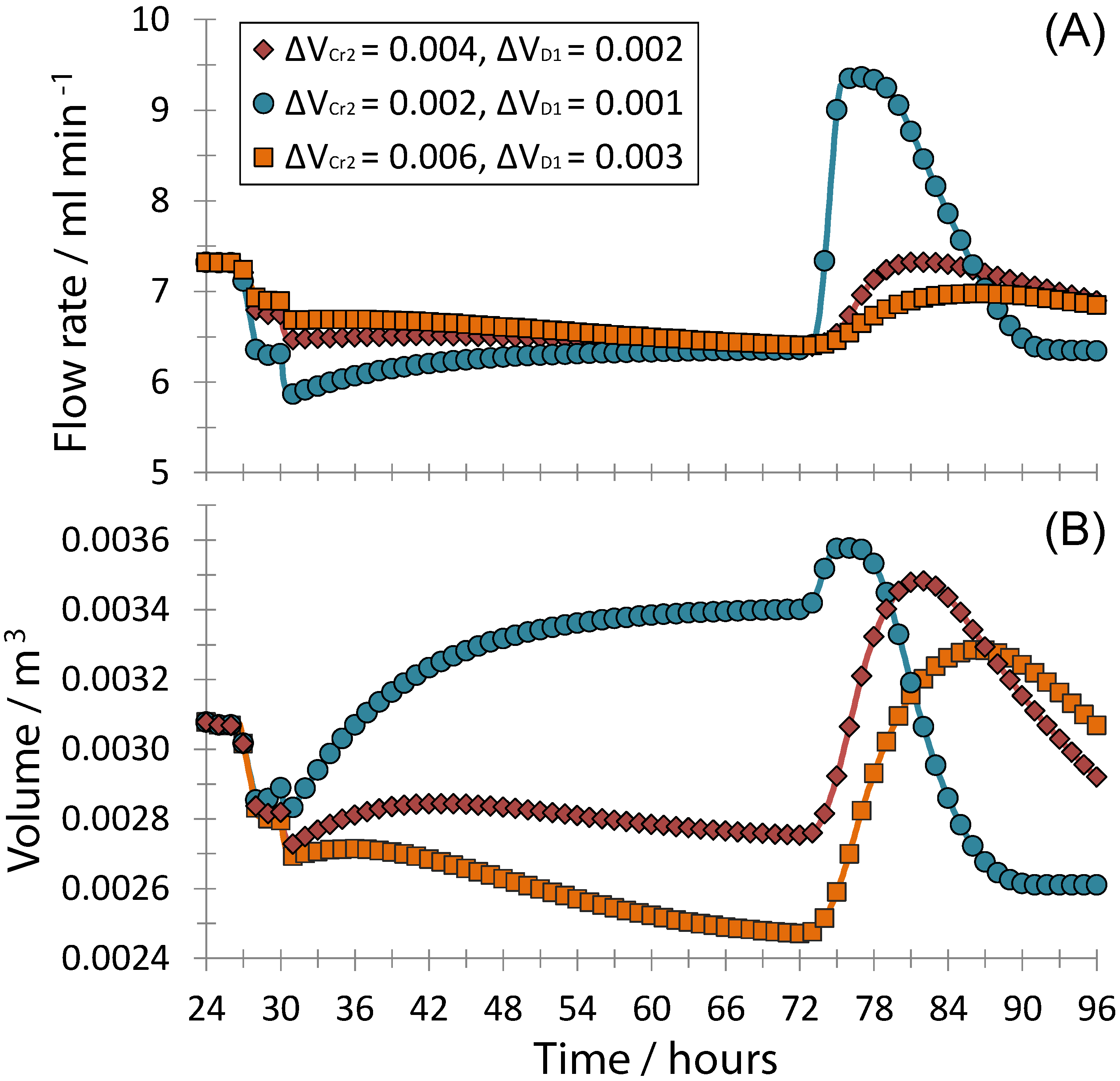
2.1. Process Description and Control Structure

A schematic representation of the studied part of the integrated continuous pharmaceutical pilot plant is given in Figure 1. A detailed description of the design of the pilot plant is presented elsewhere [45]. In this section, key elements are summarized that have a direct connection to the work presented in the present paper. An intermediate compound A is synthesized and dissolved in solvent S 1 upstream. Compound A is a reagent for the synthesis of an active pharmaceutical ingredient further downstream and is separated from solution via a cascade of two continuous crystallization steps followed by a continuous wash and filtration step. Supersaturation is generated in the crystallizers via cooling and addition of an anti-solvent ( S 2 ) to the second crystallizer, which reduces the solubility of compound A four-fold [22]. The temperature within the crystallizers is kept constant via thermostatic baths connected to the jackets of the crystallizers. Both crystallizers are equipped with level sensors (Omega LVCN414) that are calibrated to measure the total volume of the material in each crystallizer. The outlet flows of the crystallizers consist of a slurry with suspended crystals in mother liquor, which are largely separated in a continuous wash and filtration stage (W1). The purified slurry of compound A is collected in a buffer tank that can be used for dilution (D1) to which solvent can be added to dilute the slurry. The dilution tank is also equipped with a calibrated level sensor (Omega LVCN414) and an online density meter (Anton Paar DPRn 417) calibrated to measure the concentration of compound A in the tank. The outlet flow rate of the buffer tank is fed to a tubular reactor downstream for synthesis of a second intermediate compound. The variations in composition and flow rate of the material leaving the buffer tank have a significant impact on the performance of the reaction downstream. Therefore, to reduce the production of off-spec material in the complete process, a feedback concentration control loop is used to maintain the concentration of compound A in D1 close to a desired setpoint. The outlet flow rate of the buffer tank is manipulated to control the level in the tank. The variations in concentration and outlet flow rate should be minimized to maintain a constant residence time in the tubular reactor downstream. A Siemens SIMATIC PCS7 process control system was used for data archiving and implementation of the experimentally tested control loops. Such a control system allows for the flexible implementation of desired control strategies.
Figure 1. Process flowsheet of a section of a continuous pharmaceutical pilot plant that consists of two crystallizers in series (Cr1–2), a washing and filtration stage (W1), and a buffer tank that can be used for dilution (D1). The section has three automated feedback level control loops (LC1–3), two automated temperature control loops (TC1–2) and an automated feedback concentration control loop (CC1).
Processes 01 00330 g001
The tuning of the P-only feedback level controllers of the crystallizers aims to provide both stability and flow filtering to damp out fluctuations in flow rate. Therefore, the gains of the level controllers of the crystallizers, as implemented in the pilot plant, are chosen, such that the outlet flow rate of a crystallizer is approximately at the maximum flow rate when the level in the crystallizer reaches an upper limit ( V m a x ). In case a steady-state offset in level is not desired, integral action can be added. The following tuning rules are recommended for PI-ALC [46,47]:
K c = 100 % Δ V
τ c = 4 V S P K c ϕ m a x
with, for our case:
Δ V = V m a x - V S P
where K c is the controller gain, τ c is the controller integral time, V is the volume of the material in the tank and ϕ m a x is the maximum outlet flow rate. Equation (1) states that the outlet flow rate will be at a maximum value when the volume in a tank reaches the upper limit. Derivative controller action is not desired, due to the noisy signal from the level measurement devices.
Finally, a scheme that utilizes OALC is investigated. When inlet flow measurements are available, the following optimal-averaging level controller can be used [44]:
ϕ o = ϕ ˜ o + K c V - V S P + K c τ c V - V S P d t
d ϕ ˜ o d t = ϕ i - ϕ ˜ o 2 2 V m - V with V m = V m a x if d V / d t > 0 V m i n if d V / d t < 0
where ϕ i and ϕ o are the measured inlet flow rate and manipulated outlet flow rate, respectively, and V m represents a constraint on the maximum or minimum volume, depending on the direction of change of the volume, that should not be violated. The first term of Equation (4) minimizes the maximum change in outlet flow rate for a given flow imbalance, which has been augmented with equations for a PI controller. The latter does compromise on flow optimality, but also ensures that the steady state of the system will eventually move to a setpoint value, such that future disturbances can be mitigated effectively, as well. The reader is referred to McDonald et al. [44] for further details on the derivation of Equations (4) and (5). When inlet flow measurements are not available, a discrete-time optimal flow level controller could be utilized [48]. In this particular pilot plant (Figure 1), measurements of the inlet flow rate of crystallizer Cr1 are not readily available, in contrast to the measurements of the inlet flow rate of crystallizer Cr2, which can be obtained from the volumetric pumps P1 and P2. The buffer tank D1 has two inlet flow rates, i.e., stream 4 from W1 and the solvent stream (pump P5). The latter flow rate is readily available from measurements, whereas the former can be obtained from the outlet of crystallizer Cr2 (pump P3) with the assumption that the performance of the filter (W1) does not change over time. For the application of OALC, level controller LC1 utilizes P control, as was implemented in the pilot plant, and level controllers LC2 and LC3 are extended according to the schemes described by Equation (1)–(3) and, in separate simulations, by Equation (4) and (5). Note that OALC for a crystallizer is only suitable within a range in which the residence time of the crystallizer does not have a significant impact on the crystallizer performance, which calls for a conservative strategy when designing the continuous crystallization stage and for a limited allowable buffering capacity.
The tuning of the optimal-averaging level controllers requires a trade-off between flow optimality and the speed at which the level of the tank moves towards the setpoint after a disturbance, which has to be selected based on the frequency and direction of the expected disturbances. For this case study, the settings as given by Equations (1)–(3) are used as a reference for tuning the PI part of the OALC controller. In particular, the gain of the OALC controller has been taken two orders of magnitude smaller compared to the gain used for the PI-ALC controller, as given by Equation (1). Furthermore, the controller integral time has been taken as two orders of magnitude larger compared to the PI-ALC controller, as given by Equation (2). The aim is to assure that the PI part of Equation (4) does not dominate the behavior of the OALC controllers, but also that the system does move slowly to a setpoint somewhere in between the desired upper and lower limits of the tank. The resulting gains and controller integral times for the studied controllers are given in Table 1, including the nominal setpoints. Note that the setpoints for OALC correspond to the setpoints of the corresponding P level controllers, including steady-state offset.

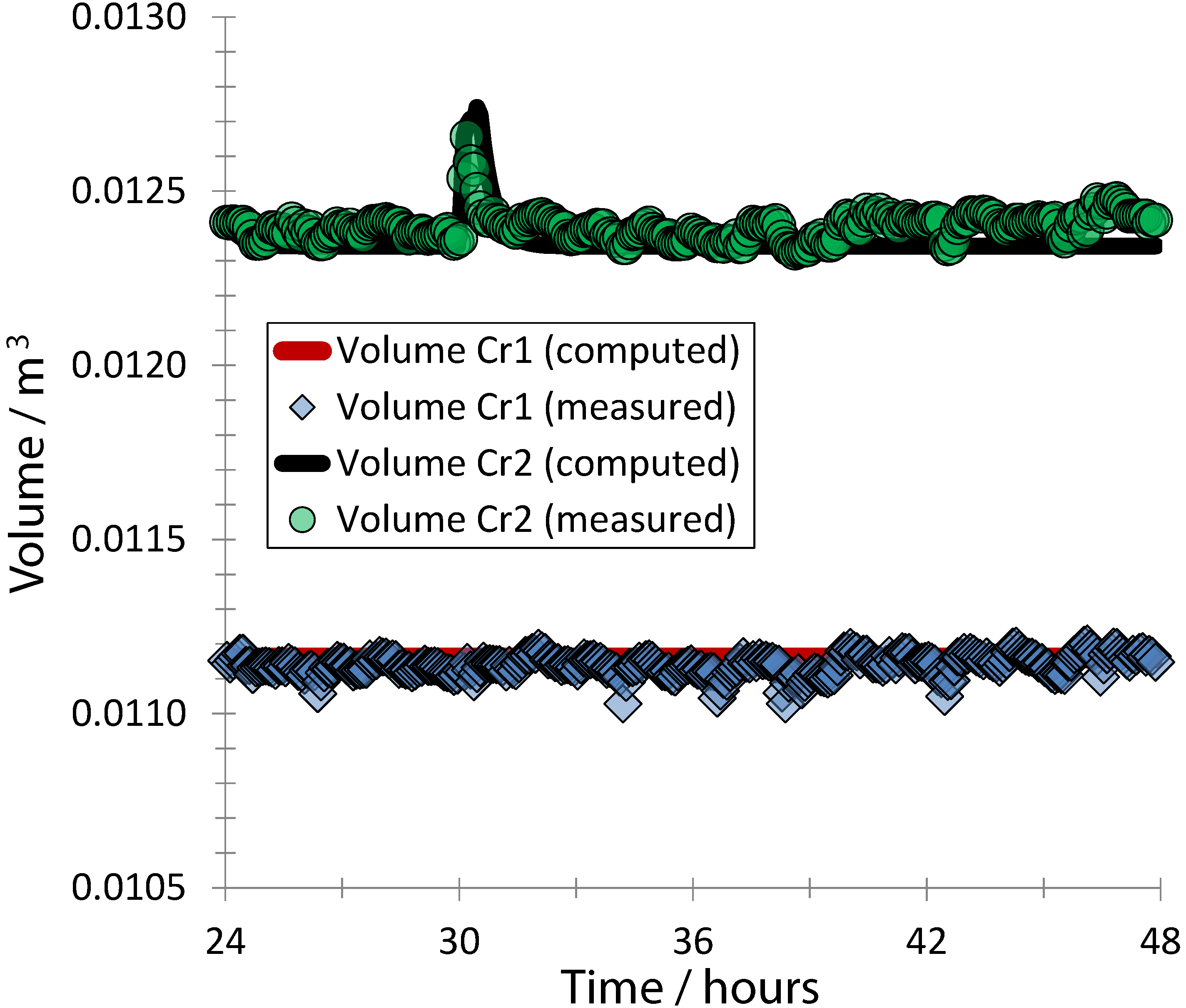
2.2. Process Modeling and Parameter Estimation

A closed-loop simulation is utilized to evaluate the effectiveness of OALC for the continuous pharmaceutical pilot plant as described in the previous section. The model equations that are relevant for the network of unit operations illustrated in Figure 1 are extracted from a plant-wide dynamic model inspired by the experimental pilot plant, as described in detail elsewhere [42]. The model contains component balances for all chemical species, moment balances to describe the dynamic evolution of the crystal size distribution and thermodynamic expressions related, for example, to solubilities. In general, the stream coming from the reactor upstream contains several impurities. However, the effect of impurities is expected to have a limited impact on the description of the overall mass balance, which is the main requirement for the present study. Therefore, the model has been simplified by considering only the component balances of the intermediate compound A and the solvents. Finally, the model has been extended with P-feedback control loops to mimic the closed-loop behavior of the pilot plant.
Several key parameters in the dynamic model were unknown and had to be estimated to ensure that the dynamic model gives an accurate description of the dynamic development of the key control objectives, i.e., the concentration of compound A in buffer tank D1 and the variations in the outlet flow rate of tank D1. Experimental data covering a period of 24 h of operation were used to estimate the unknown parameters. The time period started at t = 24 h, where t = 0 approximately corresponds to the start of the filling of the first crystallizer (Cr1). Consequently, the experimental data do not necessarily represent steady-state conditions. The experimental data contain at least one major disturbance, which was caused by blocking of the transfer line from the second crystallizer (Cr2) to the continuous washing and filtration stage (W1). Starting at t = 30 . 0 h, a number of plugging events occurred within a period of 30 min, which temporarily prevented any flow from Cr2 to W1. Note that such blocking cannot be directly observed, as volumetric pumps are used to obtain flow rates. However, the onset of plugging can easily be determined by careful examination of the measurements of the level in the tanks, and plugging events have been implemented in the model by multiplying the outlet flow rate of Cr2 with a binary variable, whose value depends on the existence of plugging for the given time. Furthermore, a setpoint change in the feedback concentration control loop (CC1) was implemented experimentally at t = 26 . 7 h to increase the concentration of compound A in buffer tank D1, as indicated in Table 1. Note that such a change in setpoint reduces the solvent flow rate going into buffer tank D1, which impacts the level and, thus, outlet flow rate of the tank.
Table 1. Tuning parameters and setpoints of the studied controllers: P, implemented in the pilot plant (proportional only); PI-ALC, implemented in a process simulator (proportional-integral tuned according to averaging level-control criteria); OALC, implemented in process simulator (optimal averaging level control).
ControllerSetpoint K c τ c Comments
LC1P 1.05 × 10 - 2 m 3 8.3 × 10 - 4 s - 1
LC2P 1.15 × 10 - 2 m 3 8.3 × 10 - 4 s - 1
PI-ALC 1.24 × 10 - 2 m 3 7.5 × 10 - 4 s - 1 5.0 × 10 3 s
OALC 1.24 × 10 - 2 m 3 7.5 × 10 - 6 s - 1 5.0 × 10 5 s V m = V S P ± 0.20 × 10 - 2 m 3
LC3P 3.00 × 10 - 3 m 3 1.7 × 10 - 3 s - 1
PI-ALC 3.08 × 10 - 3 m 3 3.3 × 10 - 4 s - 1 1.4 × 10 4 s
OALC 3.08 × 10 - 3 m 3 3.3 × 10 - 6 s - 1 1.4 × 10 6 s V m = V S P ± 0.10 × 10 - 2 m 3
CC1P 2 . 62 × 10 - 1 g/g 2.5 × 10 - 5 m 3 s - 1 w A , S P = 0.24 if t < 26.7 h
The available experimental data consist of the measured level in both crystallizers (Figure 2), the outlet flow rate of both crystallizers (Figure 3), the level in the buffer tank and the corresponding outlet flow rate (Figure 4) and the controlled concentration of compound A in buffer tank D1 with the corresponding flow rate of the solvent for dilution (Figure 5). Each data point represents the median value of a series of 30 measurements obtained within a period of 300 s. The dynamic model is implemented in JACOBIAN (RES Group, Inc.), which is a process simulator equipped with routines for parameter estimation. A maximum-likelihood objective function was used for the parameter estimation, with equal weight given to each data point. The input and output of the parameter estimation problem to fit the closed-loop dynamic model to the experimental data are presented in Table 2. These parameters characterize the properties of the material coming from the reactor upstream, the initial solid fraction in both crystallizers and the solid fraction of the slurry leaving the filter plate. The resulting dynamic model is well capable of describing the experimental data, including the dynamics during the main disturbance and the change in setpoint of the feedback concentration control loop, as illustrated in Figure 2, Figure 3, Figure 4 and Figure 5.
Figure 2. Dynamic development of the volume of crystallizers Cr1 and Cr2 (see Figure 1) for a period of 24 h describing experimentally measured data from level sensors (circles and diamonds) and a model-based computation (solid lines). The volume in each crystallizer is a controlled variable within an automated P-only feedback level control loop (LC1 and LC2). A number of plugging events occurred at t = 30.0 h in the outlet tubing of crystallizer Cr2.
Processes 01 00330 g002
Figure 3. Dynamic development of the outlet flow rates of crystallizers Cr1 and Cr2 (see Figure 1) for a period of 24 h describing experimentally measured data obtained from volumetric pumps (circles and diamonds) and a model-based computation (solid lines). The outlet flow rate of each crystallizer is a manipulated variable within an automated P-only feedback level control loop (LC1 and LC2). A number of plugging events occurred at t = 30.0 h in the outlet tubing of crystallizer Cr2.
Processes 01 00330 g003
In the next section, the model is used to investigate the potential benefit of replacing each of two P level control loops with PI-ALC level control loops and OALC, which have both been implemented in the model-based process simulator in differentiated form, with the initial condition corresponding to the measured outlet flow rate at the beginning of the investigated time interval. The simulated scenario mimics, for the first 24 h, the operation of the pilot plant, including the observed disturbances. Subsequently, the simulation is extended for another 48 h to investigate via model-based simulations the performance of the controllers when a large and temporary step change in throughput would be implemented in the process. The disturbances observed during experimental operation of the pilot plant were significant as a flow rate came to a complete stop. However, since the disturbance was relatively short, the total amount of material that was blocked was limited. Even if the OALC controller takes no corrective action, the levels of tanks are not expected to cross the upper or lower boundary. Therefore, the simulation is extended beyond the experimental period to investigate the performance of the controllers in case the levels in the tanks approach a critical value to obtain broader insight. In particular, the following step changes in the flow rate of Stream 1 are implemented in the process simulator:
F 1 = 5.0 × 10 - 4 kg s - 1 if t < 72 7.5 × 10 - 4 kg s - 1 if 72 t 76 5.0 × 10 - 4 kg s - 1 if t > 76
where F 1 is the inlet flow rate of the first crystallizer.
Figure 4. Dynamic development of the volume (A) and outlet flow rate (B) of buffer tank D1 (see Figure 1) for a period of 24 h describing experimentally measured data (diamonds) obtained from a level sensor and a volumetric pump (P6) and a model-based computation (solid lines). The outlet flow rate of buffer tank D1 is a manipulated variable, and the level is a controlled variable within an automated P-only feedback level control loop (LC3). Note that a setpoint change of a concentration control loop constructed around buffer tank D1 (CC1) at t = 26.7 h caused the volume to drop and, furthermore, a number of plugging events occurred at t = 30.0 h in the outlet tubing of crystallizer Cr2 upstream.
Processes 01 00330 g004
Table 2. Input for parameter estimation and results.
ParameterEstimated valueInitial guessBounds
Flow rate of stream 1 5.0 × 10 - 4 kg s - 1 4.9 × 10 - 4 2.8 × 10 - 6 , 8.3 × 10 - 4
Mass fraction of A in stream 1 7.4 × 10 - 2 kg / kg 1.5 × 10 - 1 6.0 × 10 - 2 , 7.5 × 10 - 1
Slurry liquid fraction at outlet of W1 2.1 × 10 - 1 kg / kg 6.5 × 10 - 1 1.0 × 10 - 1 , 8.5 × 10 - 1
Initial liquid fraction in Cr1 9.7 × 10 - 1 m 3 / m 3 8.8 × 10 - 1 6.0 × 10 - 1 , 9.8 × 10 - 1
Initial liquid fraction in Cr2 9.6 × 10 - 1 m 3 / m 3 9.6 × 10 - 1 6.0 × 10 - 1 , 9.8 × 10 - 1
Figure 5. Dynamic development of the concentration of compound A in buffer tank D1 (A) and the flow rate of solvent added to tank D1 (see Figure 1) (B) for a period of 24 h describing experimentally measured data (diamonds) obtained from an online density meter and a volumetric pump (P5) and a model-based computation (solid lines). The outlet flow rate of buffer tank D1 is a manipulated variable, and the level is a controlled variable within an automated P-only feedback level control loop (LC3). Note that a setpoint change of a concentration control loop constructed around buffer tank D1 (CC1) caused the volume to drop, and furthermore, a number of plugging events occurred at t = 30.0 h in the outlet tubing of crystallizer Cr2 upstream.
Processes 01 00330 g005

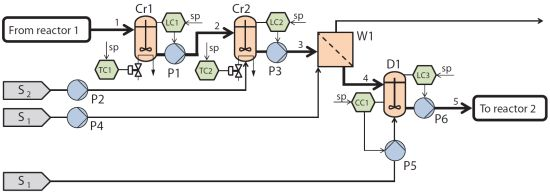
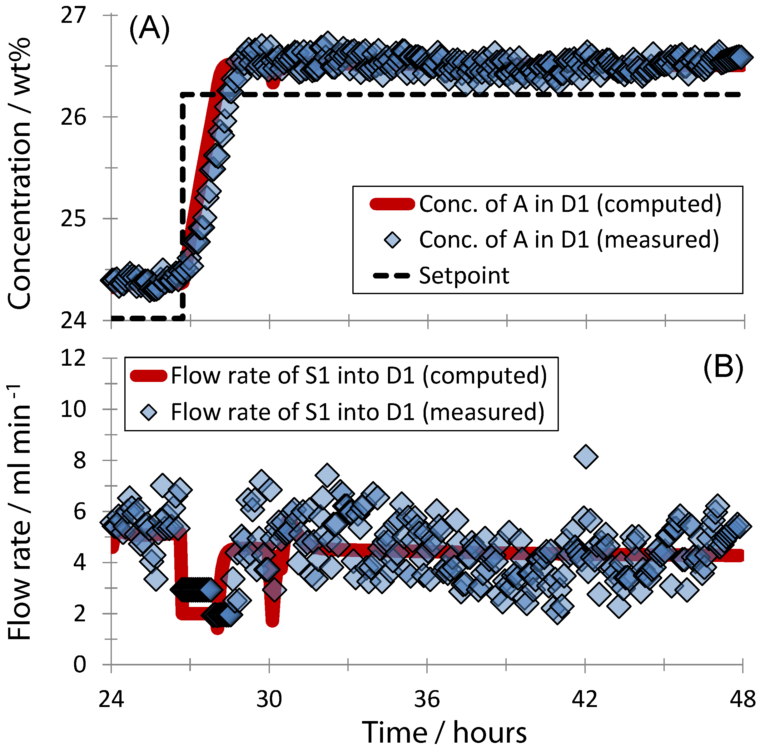
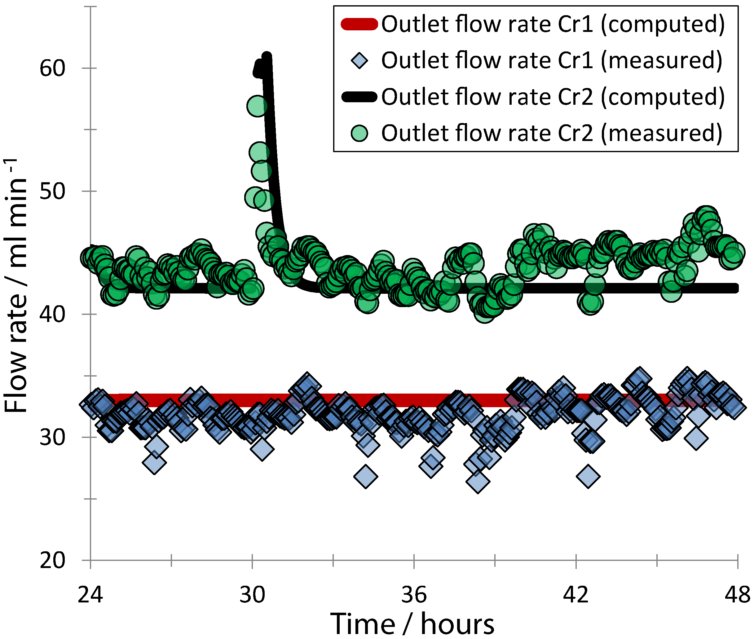
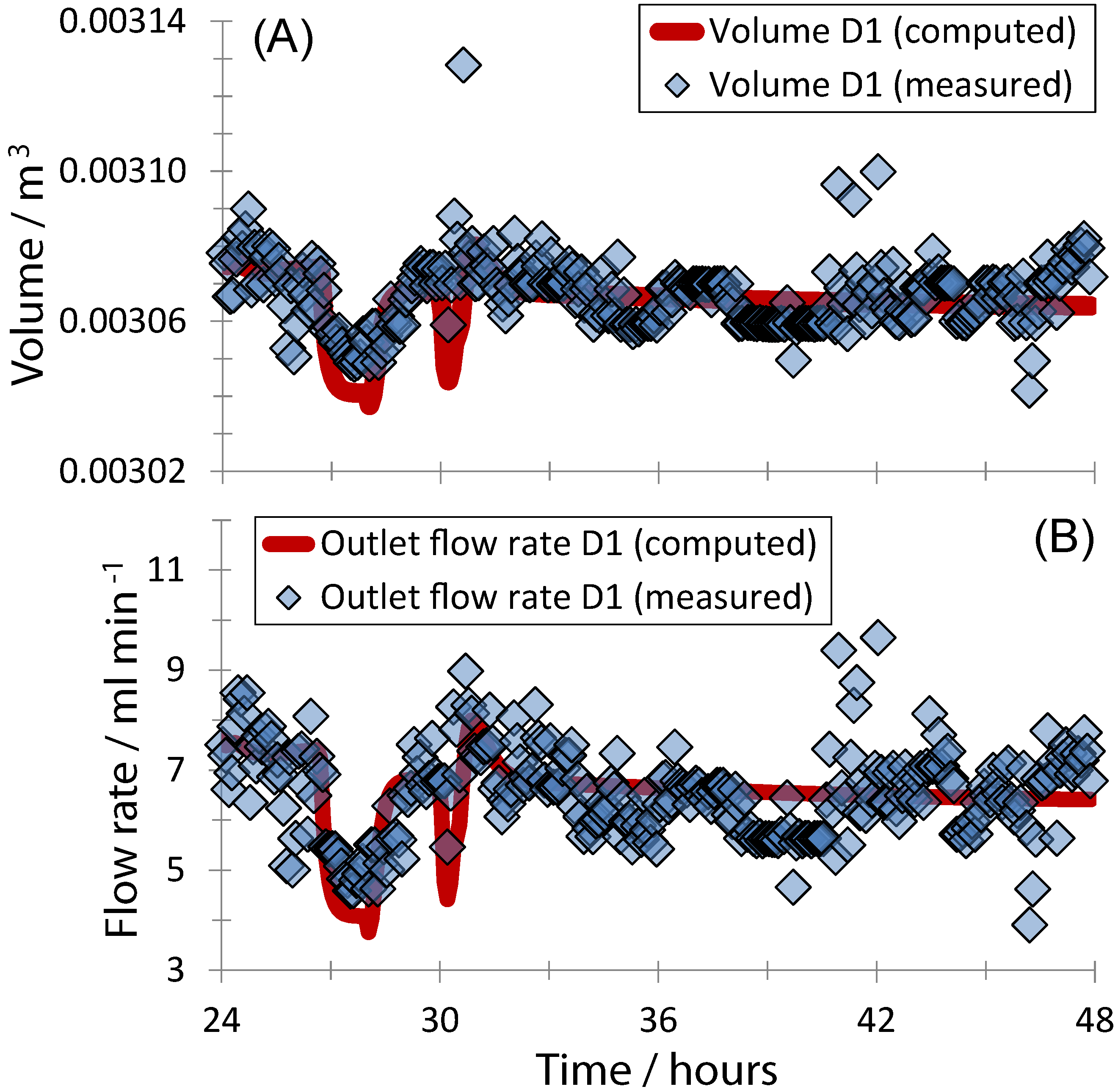
3. Results and Discussion

Figure 6 illustrates the dynamic development of the volume and the outlet flow rate of crystallizer Cr2 with P-feedback level control as implemented experimentally, with PI-ALC and with OALC. The difference in behavior is striking. Initially, after the first disturbance at t = 30.0 h, the volume for all cases rises sharply as the outlet flow rate of the crystallizer ceases (Figure 6A). In the experimentally tested case, the controller increases the outlet flow rate significantly (Figure 6B), which causes the level to return to its steady-state value within approximately 2 h. The PI-ALC controller shows a similar behavior as the P-only controller with a peak value in the outlet flow rate that is slightly higher. However, for OALC, the automated level control loop utilizes the buffering capacity of the crystallizer and brings the volume of the tank only gradually back to the setpoint. As a result, the outlet flow rate of crystallizer Cr2 hardly changes after the first disturbance hits the system (Figure 6B), which will essentially eliminate any sustained impact of this disturbance downstream. The maximum volume of the crystallizer is not yet approached after the first disturbance, which warrants the full use of buffering capacity. When the second disturbance hits the system, at t = 72.0 h, a different response can be observed. In this case, the volume of the crystallizer approaches the maximum allowable value, which results in a significant increase of the outlet flow rate in the case of OALC (Figure 6B). For all tested cases, the outlet flow rates increase temporarily with approximately 50% compared to their steady-state value. The behavior in the OALC case can be understood by the notion that the first term on the right-hand side of Equation (4) becomes dominant compared to the loosely-tuned PI part of the OALC controller when the volume approaches the upper or lower limit. In the case that only the PI part of the OALC controller would be used, the vessel would simply overflow. Note that the changes in flow rate in the case of OALC are slightly delayed compared to using only P control or PI-ALC, which causes the system to use more buffering capacity. In general, the simulation results clearly demonstrate the anticipated effectiveness of OALC to mitigate flow disturbances and to smooth changes in setpoints for the studied section of the pilot plant of a continuous pharmaceutical process.
Figure 6. Dynamic development of the volume (A) and outlet flow rate of crystallizer Cr2 (B) as predicted by a dynamic model of the process illustrated in Figure 1. The former variable is a controlled variable, and the latter variable is the manipulated variable within an automated level control loop (LC2). The black solid line (triangles) describes the simulated behavior with P-only feedback control, as was done experimentally. The blue line (circles) is the predicted behavior if PI controllers are implemented with tuning tailored for ALC. The red line (diamonds) describes the predicted behavior if OALC is implemented.
Processes 01 00330 g006
Figure 7 illustrates the dynamic development of the concentration of compound A in buffer tank D1 (controlled variable) and the flow rate of solvent into buffer tank D1 (manipulated variable) for the experimentally implemented P-feedback control for all level control loops and the expected behavior if PI-ALC or OALC were implemented for LC2 and LC3. Note that the concentration control loop itself is identical in all cases. Therefore, the behavior of all control schemes is identical in the first part of the time interval. The concentration control loop saturates at a minimum flow rate for the manipulated variable when the setpoint change is implemented and resumes to operate the closed loop when the concentration exceeds the setpoint. Since the schemes respond differently to the first disturbance occurring in the outlet flow rate of crystallizer Cr2, some differences can be observed after t = 30.0 h. Initially, the concentration, and, thus, solvent flow rate, drops sharply for all schemes, which is caused by a blocked supply of slurry from crystallizer Cr2. With P level control and PI-ALC control, the accumulated material in crystallizer Cr2 is pushed out within a relatively short amount of time to the continuous filtration and washing, which causes the concentration in the buffer tank D1 to peak slightly (Figure 7A) and, consequently, the solvent flow rate to peak, as well (Figure 7B). If OALC were implemented in the plant around the crystallizer, Cr2, the accumulated material of compound A would be pushed out at a much slower pace, which would prevent a peak in concentration of compound A in the buffer tank D1 (Figure 7A) and solvent flow rate (Figure 7B), such that steady state is approached more rapidly in the first part of the tested time interval. The behavior of the concentration control loop strongly correlates to the outlet flow rates of the crystallizer upstream for all tested controllers (Figure 6B) towards the end of the simulated period when the second disturbance hits the system, i.e., around t = 70.0 h. Note that the flow rate of solvent that is added to control the concentration of compound A also has a significant impact on the volume and, thus, on the behavior of the level control loop, of the buffer tank.
The influence of the combined effect of the disturbance upstream and the change in setpoint of the concentration control loop CC1 on the volume and outlet flow rate of buffer tank D1 is illustrated in Figure 8 for all investigated control schemes. The results show a significantly different behavior. In the case of P level control and PI-ALC, both the disturbance in flow rate from upstream and the setpoint change of the concentration control loop strongly affect the outlet flow rate of buffer tank D1. First, a sharp drop in the outlet flow rate can be observed when the change of setpoint is implemented at t = 26.7 h, which causes the inlet flow rate of the tank to decrease as a result of the decreased solvent flow rate set by the concentration control loop. Once the concentration reaches the new setpoint, the flow rate increases again to approach the new steady state. Secondly, a sharp decrease in outlet flow rate followed by a sharp increase in outlet flow rate can be observed around t = 30.0 h, which is caused by the temporarily blocked transfer line from crystallizer Cr2 to the filtration and washing stage, W1. Note that such sharp changes in the outlet flow rate directly translate to variations in the residence time of tubular Reactor 2 downstream, which would impact the synthesis of the subsequent intermediate compound and impurities. The behavior of P-only level control and PI-ALC is comparable when the second disturbance hits the system at t = 72.0 h, with the volume in the case of PI-ALC reaching a slightly higher value, because of the smaller controller gain in that case.
Figure 7. Dynamic development of the concentration of compound A in the buffer tank D1 (A) and the flow rate of solvent going into the buffer tank (B) as predicted by a dynamic model of the process illustrated in Figure 1. The former variable is a controlled variable, and the latter variable is the manipulated variable within an automated concentration control loop (CC1). The black line (triangles) describes P-feedback control implemented for crystallizer Cr2 and buffer tank D1, as was implemented experimentally. The blue line (circles) is the predicted behavior if PI-ALC feedback controllers are implemented for crystallizer Cr2 and buffer tank D1. The red line (diamonds) describes the predicted behavior if OALC were implemented for crystallizer Cr2 and buffer tank D1. The concentration control loop utilizes P-feedback control in all cases.
Processes 01 00330 g007
The expected behavior is distinctively different if OALC were implemented. For OALC, the change in setpoint of the concentration control loop does not lead to a significant drop in outlet flow rate (Figure 8B). Instead, the buffering capacity of the tank is used by reducing the volume of the tank, and a slowly increasing volume can be observed once the concentration control loop reaches its new setpoint. A similar behavior occurs when the first disturbance from upstream around t = 30.0 h causes the inlet flow rate of the tank to decrease, i.e., the volume of the material in the tank reduces significantly, while minimizing the changes in outlet flow rate. Once both inlet flow rates of buffer tank D1 are re-established at their nominal value, a gradual increase in volume to compensate for the offset can be observed until the second disturbance hits the system at t = 72.0 h. In this last part of the investigated time period, application of OALC shows a significantly lower variation in the outlet flow rate of buffer tank D1 compared to the investigated conventional schemes. This different behavior can be understood from the more gradual supply of material from upstream units (Figure 6B) and the automated use of buffering capacity in buffer tank D1 (Figure 8A). Clearly, the significantly reduced variations in outlet flow rate with OALC combined with no expected additional impact on the concentration control loop (Figure 7A) would minimize the propagation of disturbances within the studied pilot plant of an integrated continuous pharmaceutical process.
Figure 8. Dynamic development of the volume (A) and outlet flow rate of buffer tank D1 (B) as predicted by a dynamic model. The former variable is a controlled variable, and the latter variable is the manipulated variable within an automated level control loop (LC3). The black solid line (triangles) describes the simulated behavior for P-only feedback control, as was done experimentally. The blue line (circles) is the predicted behavior for PI-ALC. The red line (diamonds) describes the predicted behavior for OALC.
Processes 01 00330 g008
The central thought behind the application of OALC is to allow little control action in response to inlet disturbances when the volume of the material in a tank is sufficiently far from critical boundaries. Consequently, a more aggressive response is needed when inlet disturbances push the volume close to a critical boundary. The presented results clearly demonstrate this strong difference in behavior depending on the value of the measured volume. These observations raise the question of how to design the excess capacity of buffer tanks. Figure 9 illustrates the simulated process behavior for various allowable ranges in volume as defined by the upper and lower limit of the volume in crystallizer Cr2 and dilution tank D1. The results demonstrate that increasing the range in volume (orange squares in Figure 9) only has a modest effect on the variations in the outlet flow rate. However, upon reducing the range (blue circles in Figure 9), a distinctly different behavior can be observed with a significantly higher variation in outlet flow rate. In the latter case, the volume in the tank approaches the upper limit, and consequently, a peak value of the outlet flow rate comparable to what can be expected when applying conventional P level control or PI-ALC (Figure 8B) is observed. The results stress the attractiveness of introducing specific buffer tanks, without tight constraints on residence time and equipped with automated OALC, to damp out fluctuations in flow rate in future continuous pharmaceutical processes. In addition, exploiting an allowable range in residence time for processing units, such as crystallizers, can further strengthen automated control strategies to damp out fluctuations.
Figure 9. Dynamic development of the outlet flow rate of buffer tank D1 (A) and volume (B) as predicted by a dynamic model with OALC level control in crystallizer Cr2 and buffer tank D1 for various allowable ranges in volume. In the legend, Δ V = V m a x - V m i n , and the numbers in the legend are given in cubic meters.
Processes 01 00330 g009

4. Conclusions

The presented dynamic model gives an accurate description of the closed-loop dynamic behavior of a section of a continuous pharmaceutical pilot plant involving continuous crystallization, filtration, washing and buffering of an intermediate pharmaceutical compound, at least for the studied conditions. The studied section involves three automated level control loops and one automated concentration control loop. The experimental data included a significant disturbance in the outlet flow rate of a crystallizer and a change in the setpoint of a concentration control loop around the buffer tank. Model-based simulations of the system in which two of the experimentally implemented proportional-only feedback level controllers are exchanged with optimal-averaging level controllers showed a clear benefit of using optimal-averaging level control to automatically exploit the buffering capacity of tanks within a continuous pharmaceutical process. The model-based simulations predict a significant reduction in the variation of the flow rate leaving the buffer tank for the experimentally observed disturbances, which would result in reduced variation of the residence time of a tubular reactor downstream. The performance of optimal averaging level control, at least for the investigated conditions, also strongly outperforms the performance in the case of conventional proportional-integral control with the values for the tuning parameters tailored for averaging level control.
In general, it is expected that dynamic process models will play an important role in the design of future continuous pharmaceutical processes by, for example, judicious design of buffer tanks within a plant, as illustrated in this work, or advanced model-predictive control strategies.

Acknowledgments

Novartis International AG is acknowledged for support. The study presented in this paper is based on a pilot plant that was constructed within the Novartis-MIT Center for Continuous Manufacturing. The members of the team that developed this pilot plant are acknowledged, in particular: Soubir Basak, Erin Bell, Stephen C. Born, Louis Buchbinder, Ellen Cappo, Corinne Carland, Alyssa N. D’Antonio, Joshua Dittrich, James M.B. Evans, Ryan Hartman, Devin R. Hersey, Rachael Hogan, Bowen Huo, Anjani Jha, Ashley S. King, Tushar Kulkarni, Timur Kurzej, Aaron Lamoureux, Paul S. Madenjian, Salvatore Mascia, Sean Ogden, Ketan Pimparkar, Joel Putnam, Anna Santiso, Jose C. Sepulveda, Min Su, Daniel Tam, Mengying Tao, Kristen Talbot, Chris Testa, Justin Quon, Forrest Whitcher and Aaron Wolfe (from MIT). Michael Hogan from Siemens is acknowledged for assistance with the implementation and operation of the SIMATIC PCS 7 process control system.

Conflicts of Interest

The authors declare no conflict of interest.

References

  1. Schaber, S.D.; Gerogiorgis, D.I.; Ramachandran, R.; Evans, J.M.B.; Barton, P.I.; Trout, B.L. Economic analysis of integrated continuous and batch pharmaceutical manufacturing: A case study. Ind. Eng. Chem. Res. 2011, 50, 10083–10092. [Google Scholar] [CrossRef]
  2. Plumb, K. Continuous processing in the pharmaceutical industry: Changing the mind set. Chem. Eng. Res. Des. 2005, 83, 730–738. [Google Scholar] [CrossRef]
  3. Roberge, D.M.; Ducry, L.; Bieler, N.; Cretton, P.; Zimmermann, B. Microreactor technology: A revolution for the fine chemical and pharmaceutical industries? Chem. Eng. Technol. 2005, 28, 318–323. [Google Scholar] [CrossRef]
  4. Roberge, D.M.; Zimmermann, B.; Rainone, F.; Gottsponer, M.; Eyholzer, M.; Kockmann, N. Microreactor technology and continuous processes in the fine chemical and pharmaceutical industry: Is the revolution underway? Org. Process Res. Dev. 2008, 12, 905–910. [Google Scholar] [CrossRef]
  5. Jimenez-Gonzalez, C.; Poechlauer, P.; Broxterman, Q.B.; Yang, B.S.; Am Ende, D.; Baird, J.; Bertsch, C.; Hannah, R.E.; Dell’Orco, P.; Noorrnan, H.; et al. Key green engineering research areas for sustainable manufacturing: A perspective from pharmaceutical and fine chemicals manufacturers. Org. Process. Res. Dev. 2011, 15, 900–911. [Google Scholar] [CrossRef]
  6. LaPorte, T.L.; Wang, C. Continuous processes for the production of pharmaceutical intermediates and active pharmaceutical ingredients. Curr. Opin. Drug Discovery Dev. 2007, 10, 738–745. [Google Scholar]
  7. Kockmann, N.; Gottsponer, M.; Zimmermann, B.; Roberge, D.M. Enabling continuous-flow chemistry in microstructured devices for pharmaceutical and fine-chemical production. Chem. Eur. J. 2008, 14, 7470–7477. [Google Scholar] [CrossRef] [PubMed]
  8. Hartman, R.L.; McMullen, J.P.; Jensen, K.F. Deciding whether to go with the flow: Evaluating the merits of flow reactors for synthesis. Angew. Chem. Int. Ed. 2011, 50, 7502–7519. [Google Scholar] [CrossRef] [PubMed]
  9. Wegner, J.; Ceylan, S.; Kirschning, A. Ten key issues in modern flow chemistry. Chem. Commun. 2011, 47, 4583–4592. [Google Scholar] [CrossRef] [PubMed]
  10. Wegner, J.; Ceylan, S.; Kirschning, A. Flow chemistry— A key enabling technology for (multistep) organic synthesis. Adv. Synth. Catal. 2012, 354, 17–57. [Google Scholar] [CrossRef]
  11. Pollet, P.; Cope, E.D.; Kassner, M.K.; Charney, R.; Terett, S.H.; Richman, K.W.; Dubay, W.; Stringer, J.; Eckertt, C.A.; Liotta, C.L. Production of (S)-1-benzyl-3-diazo-2-oxopropylcarbamic acid tert-butyl ester, a diazoketone pharmaceutical intermediate, employing a small scale continuous reactor. Ind. Eng. Chem. Res. 2009, 48, 7032–7036. [Google Scholar] [CrossRef]
  12. Christensen, K.M.; Pedersen, M.J.; Dam-Johansen, K.; Holm, T.L.; Skovby, T.; Kiil, S. Design and operation of a filter reactor for continuous production of a selected pharmaceutical intermediate. Chem. Eng. Sci. 2012, 26, 111–117. [Google Scholar] [CrossRef]
  13. Chen, J.; Sarma, B.; Evans, J.M.B.; Myerson, A.S. Pharmaceutical crystallization. Cryst. Growth Des. 2011, 11, 887–895. [Google Scholar] [CrossRef]
  14. Griffin, D.W.; Mellichamp, D.A.; Doherty, M.F. Reducing the mean size of API crystals by continuous manufacturing with product classification and recycle. Chem. Eng. Sci. 2010, 65, 5770–5780. [Google Scholar] [CrossRef]
  15. Wong, S.Y.; Tatusko, A.P.; Trout, B.L.; Myerson, A.S. Development of continuous crystallization processes using a single-stage mixed-suspension, mixed-product removal crystallizer with recycle. Cryst. Growth Des. 2012, 12, 5701–5707. [Google Scholar] [CrossRef]
  16. Alvarez, A.J.; Myerson, A.S. Continuous plug flow crystallization of pharmaceutical compounds. Cryst. Growth Des. 2010, 10, 2219–2228. [Google Scholar] [CrossRef]
  17. Alvarez, A.J.; Singh, A.; Myerson, A.S. Crystallization of Cyclosporine in a multistage continuous MSMPR crystallizer. Cryst. Growth Des. 2011, 11, 4392–4400. [Google Scholar] [CrossRef]
  18. Lawton, S.; Steele, G.; Shering, P.; Zhao, L.H.; Laird, I.; Ni, X.W. Continuous crystallization of pharmaceuticals using a continuous oscillatory baffled crystallizer. Org. Process Res. Dev. 2009, 13, 1357–1363. [Google Scholar] [CrossRef]
  19. Eder, R.J.P.; Schmitt, E.K.; Grill, J.; Radl, S.; Gruber-Woelfler, H.; Khinast, J.G. Seed loading effects on the mean crystal size of acetylsalicylic acid in a continuous-flow crystallization device. Cryst. Res. Technol. 2011, 46, 227–237. [Google Scholar] [CrossRef]
  20. Eder, R.J.P.; Schrank, S.; Besenhard, M.O.; Roblegg, E.; Gruber-Woelfler, H.; Khinast, J.G. Continuous sonocrystallization of acetylsalicylic acid (ASA): Control of crystal size. Cryst. Growth Des. 2012, 12, 4733–4738. [Google Scholar] [CrossRef]
  21. Quon, J.; Zhang, H.; Alvarez, A.J.; Evans, J.M.B.; Myerson, A.S.; Trout, B.L. Continuous crystallization of aliskiren hemifumarate. Org. Process Res. Dev. 2012, 12, 3036–3044. [Google Scholar] [CrossRef]
  22. Zhang, H.; Quon, J.; Alvarez, A.J.; Evans, J.M.B.; Myerson, A.S.; Trout, B.L. Development of continuous anti-solvent/cooling crystallization process using cascaded mixed suspension, mixed product removal crystallizers. Org. Process Res. Dev. 2012, 16, 915–924. [Google Scholar] [CrossRef]
  23. Mortier, S.T.F.C.; De Beer, T.; Gernaey, K.V.; Vercruysse, J.; Fonteyne, M.; Remon, J.P.; Vervaet, C.; Nopens, I. Mechanistic modelling of the drying behaviour of single pharmaceutical granules. Eur. J. Pharm. Biopharm. 2012, 80, 682–689. [Google Scholar] [CrossRef] [PubMed]
  24. Gonnissen, Y.; Remon, J.P.; Vervaet, C. Development of directly compressible powders via co-spray drying. Eur. J. Pharm. Biopharm. 2007, 67, 220–226. [Google Scholar] [CrossRef] [PubMed]
  25. Gonnissen, Y.; Goncalves, S.I.V.; De Geest, B.G.; Remon, J.P.; Vervaet, C. Process design applied to optimise a directly compressible powder produced via a continuous manufacturing process. Eur. J. Pharm. Biopharm. 2008, 68, 760–770. [Google Scholar] [CrossRef] [PubMed]
  26. Wang, M.; Rutledge, G.C.; Myerson, A.S.; Trout, B.L. Production and characterization of carbamazepine nanocrystals by electrospraying for continuous pharmaceutical manufacturing. J. Pharm. Sci. 2012, 101, 1178–1188. [Google Scholar] [CrossRef] [PubMed]
  27. Brettmann, B.; Bell, E.; Myerson, A.; Trout, B. Solid-state NMR characterization of high-loading solid solutions of API and excipients formed by electrospinning. J. Pharm. Sci. 2012, 101, 1538–1545. [Google Scholar] [CrossRef] [PubMed]
  28. Brettmann, B.K.; Cheng, K.; Myerson, A.S.; Trout, B.L. Electrospun formulations containing crystalline active pharmaceutical ingredients. Pharm. Res. 2013, 30, 238–246. [Google Scholar] [CrossRef] [PubMed]
  29. Dubey, A.; Vanarase, A.U.; Muzzio, F.J. Impact of process parameters on critical performance attributes of a continuous blender A DEM-based study. AIChE J. 2012, 58, 3676–3684. [Google Scholar] [CrossRef]
  30. Dubey, A.; Sarkar, A.; Ierapetritou, M.; Wassgren, C.R.; Muzzio, F.J. Computational approaches for studying the granular dynamics of continuous blending processes, 1-DEM based methods. Macromol. Mater. Eng. 2011, 296, 290–307. [Google Scholar] [CrossRef]
  31. Portillo, P.M.; Ierapetritou, M.G.; Muzzio, F.J. Effects of rotation rate, mixing angle, and cohesion in two continuous powder mixers–A statistical approach. Powder Technol. 2009, 194, 217–227. [Google Scholar] [CrossRef]
  32. Hamdan, I.M.; Reklaitis, G.V.; Venkatasubramanian, V. Exceptional events management applied to roller compaction of pharmaceutical powders. J. Pharm. Innov. 2010, 5, 147–160. [Google Scholar] [CrossRef]
  33. Singh, R.; Ierapetritou, M.; Ramachandran, R. An engineering study on the enhanced control and operation of continuous manufacturing of pharmaceutical tablets via roller compaction. Int. J. Pharm. 2012, 438, 307–326. [Google Scholar] [CrossRef] [PubMed]
  34. Wiles, C.; Watts, P. Continuous flow reactors: A perspective. Green Chem. 2012, 14, 38–54. [Google Scholar] [CrossRef]
  35. Poechlauer, P.; Manley, J.; Broxterman, R.; Gregertsen, B.; Ridemark, M. Continuous processing in the manufacture of active pharmaceutical ingredients and finished dosage forms: An industry perspective. Org. Process Res. Dev. 2012, 16, 1586–1590. [Google Scholar] [CrossRef]
  36. Singh, R.; Gernaey, K.V.; Gani, R. Model-based computer-aided framework for design of process monitoring and analysis systems. Comput. Chem. Eng. 2009, 33, 22–42. [Google Scholar] [CrossRef]
  37. Gernaey, K.V.; Cervera-Padrell, A.E.; Woodley, J.M. A perspective on PSE in pharmaceutical process development and innovation. Comput. Chem. Eng. 2012, 42, 15–29. [Google Scholar] [CrossRef]
  38. Cervera-Padrell, A.E.; Skovby, T.; Kiil, S.; Gani, R.; Gernaey, K.V. Active pharmaceutical ingredient (API) production involving continuous processes—A process systems engineering (PSE)-assisted design framework. Eur. J. Pharm. Biopharm. 2012, 82, 437–456. [Google Scholar] [CrossRef] [PubMed]
  39. Gernaey, K.V.; Gani, R. A model-based systems approach to pharmaceutical product-process design and analysis. Chem. Eng. Sci. 2010, 65, 5757–5769. [Google Scholar] [CrossRef]
  40. Gernaey, K.V.; Cervera-Padrell, A.E.; Woodley, J.M. Development of continuous pharmaceutical production processes supported by process systems engineering methods and tools. Future Med. Chem. 2012, 4, 1371–1374. [Google Scholar] [CrossRef] [PubMed]
  41. Boukouvala, F.; Niotis, V.; Ramachandran, R.; Muzzio, F.J.; Ierapetritou, M.G. An integrated approach for dynamic flowsheet modeling and sensitivity analysis of a continuous tablet manufacturing process. Comput. Chem. Eng. 2012, 42, 30–47. [Google Scholar] [CrossRef]
  42. Benyahia, B.; Lakerveld, R.; Barton, P.I. A plant-wide dynamic model of a continuous pharmaceutical process. Ind. Eng. Chem. Res. 2012, 51, 15393–15412. [Google Scholar] [CrossRef]
  43. Lakerveld, R.; Benyahia, B.; Braatz, R.D.; Barton, P.I. Model-based design of a plant-wide control strategy for a continuous pharmaceutical plant. AIChE J. 2013, 59, 3671–3685. [Google Scholar] [CrossRef] [Green Version]
  44. McDonald, K.A.; McAvoy, T.J.; Tits, A. Optimal averaging level control. AIChE J. 1986, 32, 75–86. [Google Scholar] [CrossRef]
  45. Mascia, S.; Heider, P.L.; Zhang, H.; Lakerveld, R.; Benyahia, B.; Barton, P.I.; Braatz, R.D.; Cooney, C.L.; Evans, J.M.B.; Jamison, T.F.; et al. End-to-end continuous manufacturing of pharmaceuticals: Integrated synthesis, purification, and final dosage formation. Angew. Chem. Int. Ed. 2013, 52, 12359–12363. [Google Scholar] [CrossRef] [PubMed]
  46. Seborg, D.E.; Edgar, T.F.; Mellichamp, D.A.; Doyle, F.J., III. Process Dynamics and Control, 3rd ed.; John Wiley & Sons: Hoboken, NJ, USA, 2011; pp. 107–108. [Google Scholar]
  47. St. Clair, D.W. Controller Tuning and Control Loop Performance: “PID without the Math”, 2nd ed.; Straight-line Control Co. Inc.: Newark, NJ, USA, 1993. [Google Scholar]
  48. Campo, P.J.; Morari, M. Model predictive optimal averaging level control. AIChE J. 1989, 35, 579–591. [Google Scholar] [CrossRef]

