1. Introduction
As global energy demand rises and climate change concerns grow ever larger, the importance of using energy more efficiently continues to increase. One method of improving energy efficiency of a complex process is to create an accurate system model, and then use optimization algorithms to determine more efficient operating strategies for the system. This is especially true of building systems, which consume nearly 40% of the primary energy in the United States [
1].
Depending on a building’s heating ventilation and air conditioning (HVAC) system, a building may require heating and cooling year round. In the summer, air may be cooled to lower than required room temperatures in order to remove humidity, and then reheated to bring it back up to the desired temperature. In the winter, thermal zones in the middle of large buildings require cooling because they are not exposed to ambient conditions, thus, the thermal needs are driven by the internal gains of the zone. Chillers are generally used to meet building cooling needs, and boilers are often used to provide heating.
Steady-state chiller models have been used extensively for a variety of chiller types and sizes. Chiller models can be based on first-principles [
2,
3] or on purely empirical relationships, such as neural networks [
4]. Often, models developed for one chiller work for other chiller types. For example, in [
5], the authors found that model equations developed for reciprocating and absorption chillers also worked very well for centrifugal chillers. Lee
et al. [
6] identified eleven different centrifugal chiller models that have been used in the literature:
- ●
Simple linear regression model
- ●
Bi-quadratic regression model
- ●
Multivariate polynomial regression model
- ●
Simpler multivariate polynomial regression model
- ●
DOE-2 model
- ●
Modified DOE-2 model
- ●
Gordon-Ng universal model (based on the evaporator inlet water temperature)
- ●
Gordon-Ng universal model (based on the evaporator outlet water temperature) *
- ●
Modified Gordon-Ng universal model
- ●
Gordon-Ng simplified model
- ●
Lee simplified model
- ●
* This model is used in the current work.
All necessary equations for each model are included in Lee
et al. [
6], thus, they will not be reproduced here. In comparing the different models against 2401 chiller datasets they find that most chiller models perform well under all scenarios, including the four Gordon-Ng models, which are the models considered in this paper.
Chiller models have been used to determine the best operation conditions of a chiller. For example, Ng
et al. [
7] used a thermodynamic chiller model to determine the optimal operating points of a chiller. This allows chillers to operate more efficiently and can bring substantial savings in operating costs. It also has the potential to increase the chiller lifetime by avoiding operating regions that more quickly degrade the chiller.
Chillers can be used in conjunction with thermal energy storage (TES) to further improve system efficiency and reduce costs. Thermal energy storage is the storage of thermal energy (hot or cold) in some medium. Hot storage is used in applications such as district heating systems, where warm water is stored in large tanks, or in a concentrating solar power system, where solar energy is stored in the form of molten salts or synthetic oils. Cold storage is most commonly used for cooling buildings or district cooling networks where the cooling energy is stored as chilled water or ice. Thermal storage has been identified as a cost-effective way to reduce required thermal or electric equipment capacities (such as chillers or turbines) [
8,
9] and to reduce annual energy costs [
10].
Table 1.
Nomenclature.
| Symbol | Description | Units |
|---|
| Di | Total cooling demand for ith hour | kW |
| Ei | Amount of stored thermal energy at ith hour | kWh |
| Emax | Maximum capacity of the TES tank | kWh |
| Lj | Lower bound on the cooling load on jth chiller | kW |
| PAUX, ik | Power consumed by the auxiliary equipment at kth station at ith hour | kW |
| PStation, ik | Total power consumed by kth chilling station at ith hour | kW |
| Pij | Electric power consumption of the jth chiller at ith hour | kW |
| Rmax | Maximum charging/discharging rate of TES tank | kW |
![Processes 01 00312 i001]() | Condenser water inlet temperature at ith hour | K |
![Processes 01 00312 i002]() | Chilled water outlet temperature | K |
| Uj | Upper bound on the cooling load on jth chiller | kW |
| Xij | Cooling load on jth chiller at ith hour | kW |
| Mc,j | Condenser heat exchanger coefficient of the jth chiller | W K−1 |
| Me,j | Evaporator heat exchanger coefficient of the jth chiller | W K−1 |
| qc,j | Internal condenser heat loss rate in the jth centrifugal chiller | kW |
| qe,j | Internal evaporator heat loss rate in the jth centrifugal chiller | kW |
| γi | Real-time market rate of electric energy at ith hour | $/kWh |
| δij | Binary variable representing on or off status of jth chiller at ith hour by having the value of 0 or 1 respectively | Dimensionless |
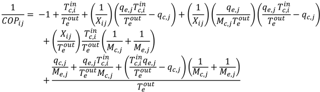
| COPij | Coefficient of performance of the jth chiller at ith hour | Dimensionless |
| DBTi | Dry bulb temperature at ith hour | K |
| r | Number of cooling stations | Dimensionless |
| mk | Total number of chillers upto the kth station; m0 = 0, mr = M | Dimensionless |
| M | Total number of chillers | Dimensionless |
| n | Number of hours in the optimization horizon | Dimensionless |
| RHi | Relative humidity at ith hour | Dimensionless |
| WBTi | Wet bulb temperature at ith hour | K |
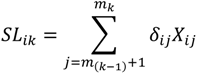
| SLik | Total cooling load at kth station at ith hour | kW |
| α | Penalty coefficient | $/kW |
| Pdata | Actual power consumed by the cooling system operation in a day | MWh |
| Popt | Estimated power consumption by the cooling system operation in a day for the cooling load profile resulted from solving optimization | MWh |
Modeling and optimizing a system that has both a large number of chillers or boilers and TES leads to complex optimization problems with binary or integer variables. For example, Tveit
et al. [
11] optimized a system that included long-term thermal storage in a district heating system. The problem was solved as a multi-period mixed integer nonlinear program (MINLP). Söderman [
12] considered the design and operation of a district cooling system with thermal energy storage in the form of cold water. He used linear models and was able to formulate and solve the problem as a mixed integer linear program (MILP).
In this paper the cooling system of a large campus is modeled and optimal chilling loads are determined. As the modeling is based on real data, the optimal results are able to be benchmarked against an actual operating strategy in order to accurately assess the potential of the optimization scheme. The optimization formulation includes a penalty term to account for the cost of switching chillers on and off. Additionally, this paper is unique in that it also considers the benefits of using a thermal energy storage system to perform optimal load shifting in a wholesale electricity market using actual wholesale market prices. All the symbols used in this paper are defined in
Table 1.
2. System Overview
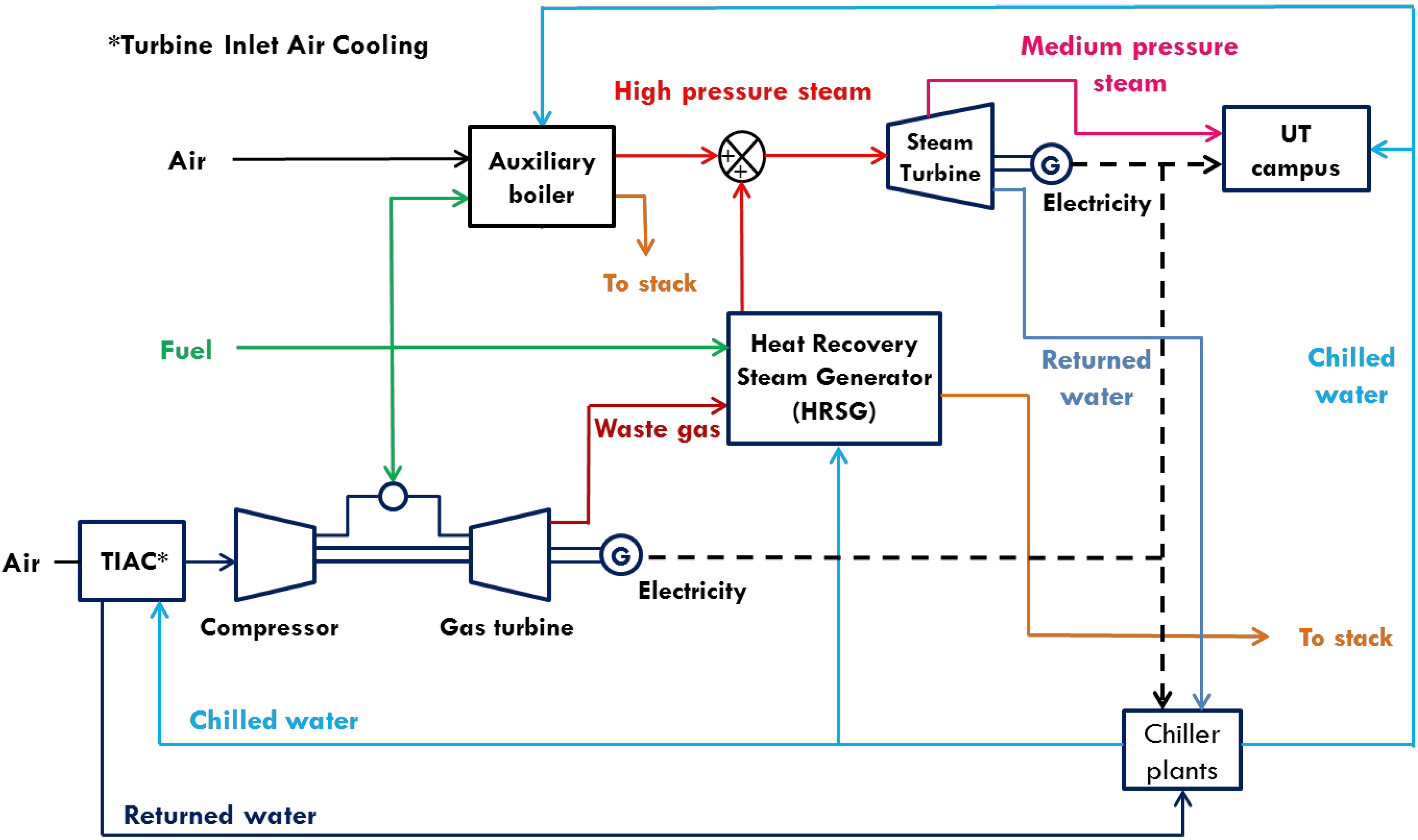
The University of Texas at Austin (UT Austin) has its own independent cogeneration based power plant (see
Figure 1 for process schematic), which generates power typically at about 6 ¢/kWh.
Figure 1.
Simplified schematic of the Hal C. Weaver power plant complex at the University of Texas at Austin.
Figure 1.
Simplified schematic of the Hal C. Weaver power plant complex at the University of Texas at Austin.
About a third of the power generated by the power plant is used by the cooling system; primarily by chillers, cooling towers, and pumps. UT Austin has a large district cooling network to meet the cooling demands of the entire campus. The cooling system includes three chiller plants (also called cooling stations) and a four million gallon (15,100 m3) chilled water thermal energy storage tank. This tank has a storage capacity of 39,000 ton-hr (494 GJ). The tank can be filled with chilled water during the night and then discharged during the day when demand for cooling is highest. This cooling system serves over 160 buildings with approximately 17 million square feet (1.6 million m2) of space. The three active cooling stations are numbered as Station 3, Station 5, and Station 6 (Stations 1, 2, and 4 have either been decommissioned or are not currently in use). Each station includes three centrifugal chillers, a set of cooling towers, condenser water pumps, and chilled water pumps. Station 6 has variable frequency drives installed on all equipment. The chillers in any Station X are named as X.1, X.2, and X.3.
4. Multi-Period Cooling System Optimization
The existing strategy for operating two out of the three chiller plants at UT Austin (plant 3 and plant 5), which do not have motors with variable speed drives, is based on heuristics and operators’ discretion drives, and hence may be suboptimal. Chiller plant 6 has variable speed drives (VSD) installed on all its equipment and the decisions regarding its chiller loads are based on equal marginal performance principal (EMPP) [
13]. EMPP is an unconstrained gradient-based optimal control strategy. Therefore, the optimal chiller load values at an instant are expected to be dependent on the previous operating values of chiller loads. Moreover, the decision to turn chillers on and off is taken based on the rise and fall in cooling demand and not on the varying efficiencies of individual chillers.
It is proposed in this paper that independent optimization problems solved at regular intervals with wisely chosen initial conditions and satisfying constraints should give better results for all chiller plants, as compared to the current operating strategy. The optimal chiller loading problem is formulated in two ways, as described in detail in the following subsections. First, it is solved as hourly independent steady state optimization problems where the cooling system is considered without any thermal storage. Next, the thermal storage is included as part of the cooling system, and the time span of one optimization problem is expanded to 24 h in order to take advantage of the flexibility to shift cooling loads.
4.1. Cooling System Optimization without Storage
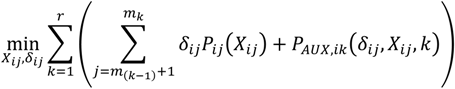
Optimal chiller loading is solved as a multi-period static optimization problem. The objective of this problem is to minimize the total power consumed by the cooling system. This objective is achieved by optimizing the cooling load distribution among various chillers operating in parallel. There are two decision variables for each chiller—the individual chiller load and a binary variable defining the chiller state,
i.e., on or off. Therefore, for a total of
M chillers, the static optimization problem has 2
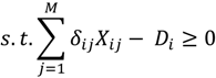
M decision variables, half of which are binary. The optimization problem also includes an inequality constraint requiring the chillers to satisfy the total cooling load. Mathematically, the static optimization formulation for any
ith hour can be represented with the following set of equations:
In Equation (4a), Pij and PAUX,ik are defined by Equations (1b) and (2a) respectively.
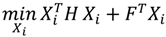
For a system of M chillers, the total number of possible
δij sets at a given time (constant
i) is (2
M − 1). For any fixed set of
δij, the objective function can be written as quadratic programming (QP) formulation,
i.e., in the form of the following equation, due to the nature of models.
The hessian of matrix H was verified to be positive definite for all possible cases. Hence, the optimization problem (Equation (4) with a fixed set of δij) was a non-linear convex formulation. It was solved for each of the (29 − 1 = 511) possible sets of δij in MATLAB using the sequential quadratic programming (SQP) algorithm to obtain a unique global solution always. The case resulting in the least value of the objective function was accepted as the optimal solution. The total time taken by the MATLAB algorithm in solving this QP for 511 cases in order to obtain the optimal solution varied between 1 and 2 s.
4.2. Cooling System Optimization with Storage
Another goal of this research is to determine the advantage of using thermal energy storage (TES) with a large scale cooling system. Thermal storage is used to shift cooling load between different hours of the day. The extra chilled water generated during a given low-demand hour is sent to the storage tank and is retrieved during a high-demand hour to satisfy the extra cooling demand. The use of TES gives flexibility to shift cooling load across time periods and, hence, to use the most efficient chillers more often and the least efficient chillers less often. The addition of storage also makes the optimization problem dynamic because the current state of the storage depends on previous states. Optimal operation of the cooling system with storage should lead to additional energy savings.
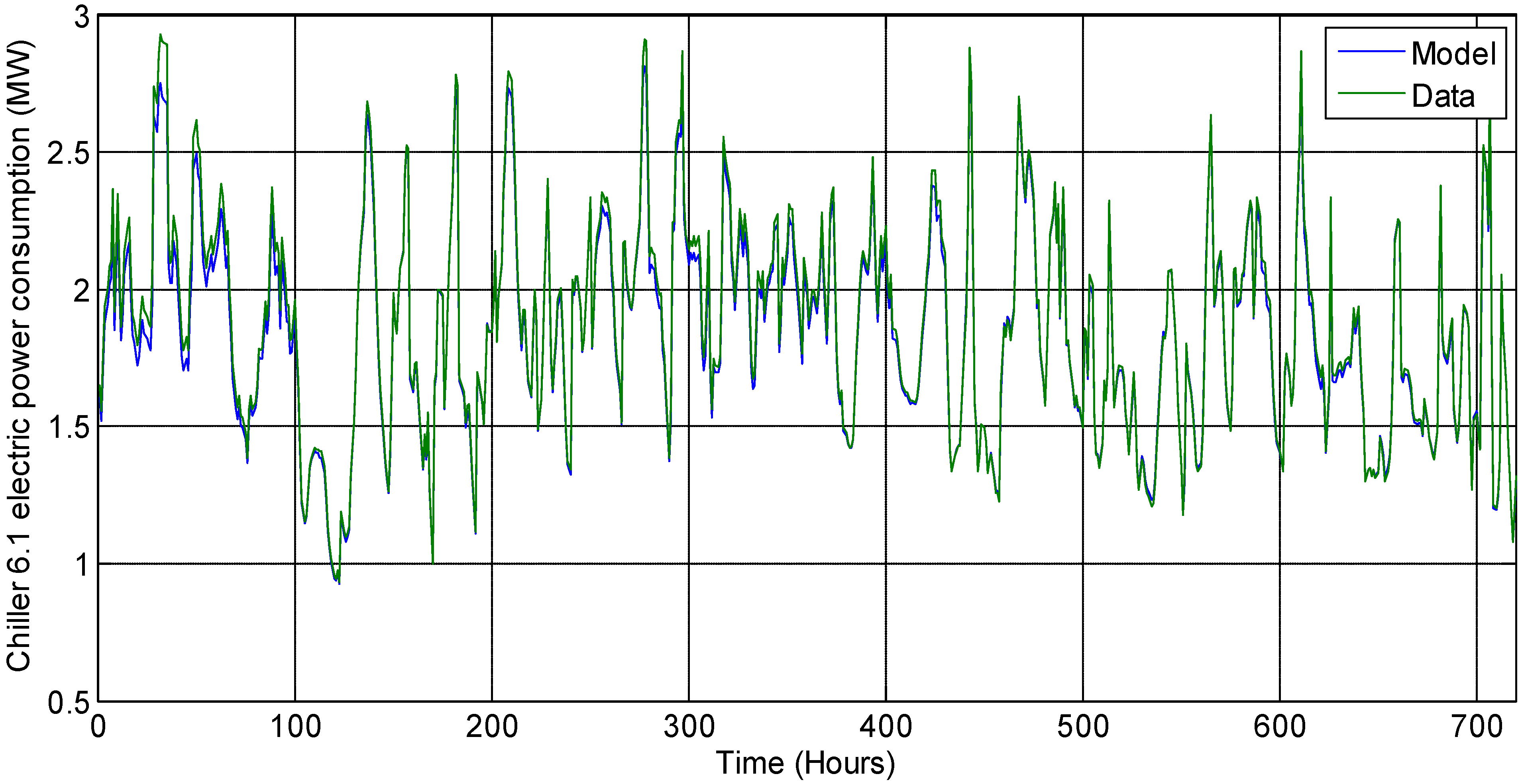
Apart from savings on energy cost, the use of TES may benefit the chiller plant operation by flattening the cooling load profile over a day. Typically the total cooling load is at a lower level during the night and increases after sunrise and when occupants arrive on campus. After reaching a peak load, it again decreases in the evening. Depending on the fluctuations in the ambient temperature and building occupancy, this cooling load profile sometimes undergoes many fluctuations during the day (
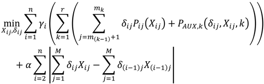
Figure 4). These fluctuations in the cooling load profile translate to frequent switching on and off of chillers, cooling towers, and pumps. There are energy losses or inefficiencies associated with the transient operation of chiller plant equipment. These losses are not accounted for while solving the static multi-period hourly chiller optimization problems, which are assumed to be independent from each other. Fluctuations in the cooling load profile also cause greater wear on chillers in addition to heat losses. However, while solving an optimization problem with thermal energy storage, we can address the issue of frequent cold starts in plant operation by adding a penalty cost to the objective function. This penalty cost is proportional to the sum of absolute difference between the total plant cooling load values at any two consecutive hours. The proportionality constant α (referred to as the penalty coefficient) can have an arbitrary positive value. The penalty cost is added to the objective function to limit the amount of fluctuations in the cooling load profile in the optimal solution. Hence, it is expected to reduce the number of times any chiller is turned on or off.
Figure 4.
Hourly campus cooling load values (left axis) and ambient wetbulb temperature values (right axis) over 24 h period. This data is from 11 July 2012. It serves as an example for days with more than one maxima in the cooling load profile.
Figure 4.
Hourly campus cooling load values (left axis) and ambient wetbulb temperature values (right axis) over 24 h period. This data is from 11 July 2012. It serves as an example for days with more than one maxima in the cooling load profile.
Therefore, optimization with thermal energy storage aims at two improvements in the energy efficiency by reducing the energy cost associated with (a) operating the chillers; and (b) frequent cold starts.
The optimization problem formulation for a time span over
n hours can be represented mathematically as follows:
An important thing to note is that the objective of this problem (Equation (6a)) is to minimize the total cost ($) of power. On the other hand, the objective of the optimization problem without storage (Equation (4a)) was to minimize the total power consumed (kWh) by the cooling system.
This optimization problem is solved in two stages [
14]. In the first stage, the total cooling load is optimally distributed among
n discrete time periods (hours), while satisfying the cooling demand at each hour with the help of thermal energy storage. In the second stage, the cooling load on
ith hour is optimally distributed among
M independent chillers having different model characteristics, which is equivalent to the optimization problem without storage. Hence, the optimization problem with storage consists of
n number of static optimization problems without storage.
5. Results and Discussion
This section discusses the optimization results from several different cases. The cooling process system optimization problem was solved for the duration of a year. The problem of optimization without storage was solved hourly while optimization with storage was solved daily.
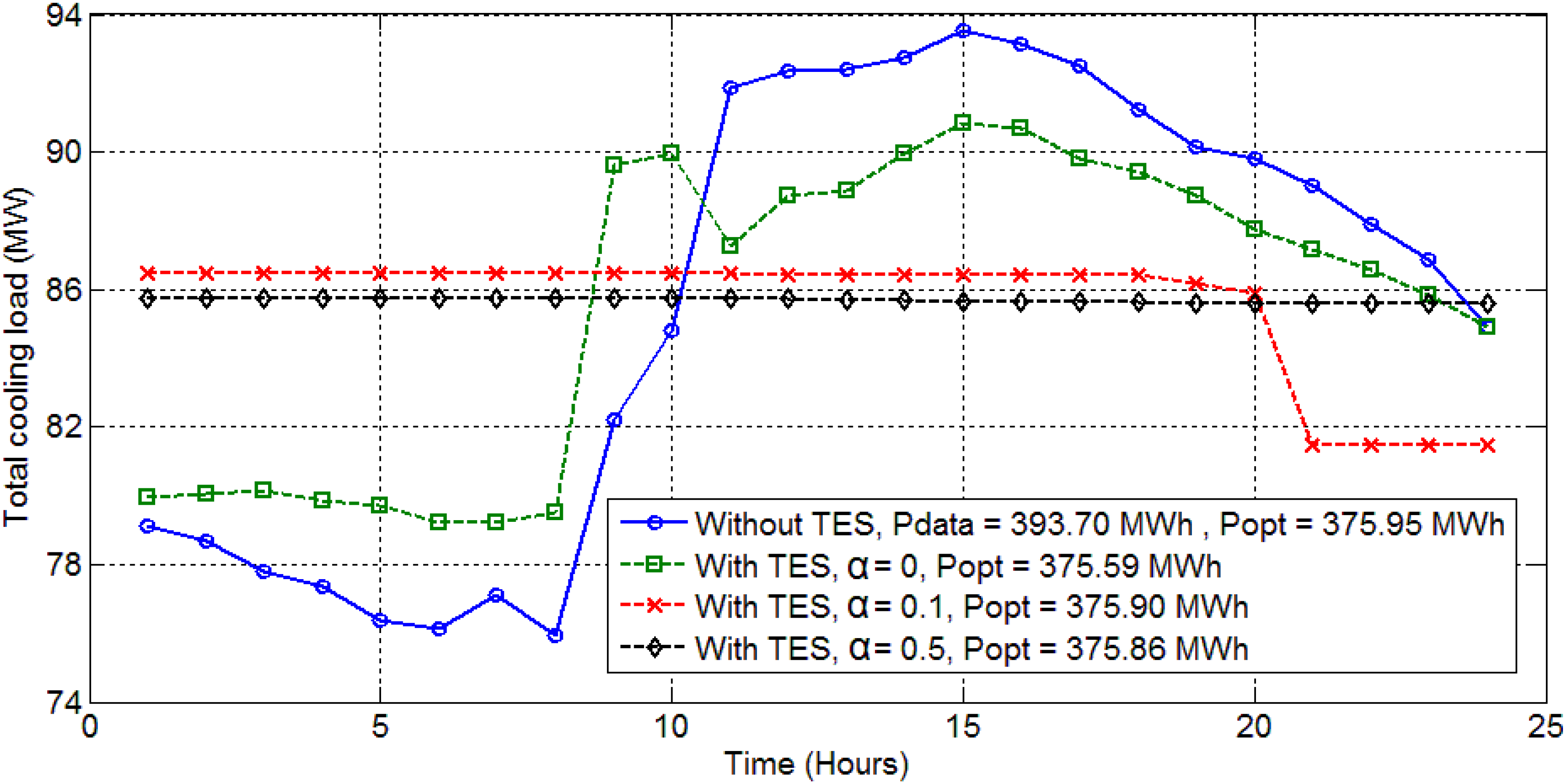
Hourly static optimization problems were solved for a year for the cooling system without storage. The model’s predicted optimal power consumption values were compared against real data collected from the UT chiller plants. The results predict energy savings as high as 40% for a single time step which is of one hour. The average energy savings over 8784 h of a year is predicted to be 8.57%. In an absolute sense, the static optimal chiller loading could save about 8.1 GWh (~$486,000) over the year in 2012. In the current operation, the cooling loads for six out of nine chillers (Stations 3 and 5) are determined based on operators’ discretion and some heuristics that are easy to follow but not based on optimal operation. The cooling loads for chillers in Station 6 are determined based on a gradient based control strategy [
13], which is expected to converge at the nearest local minima. On the other hand, the proposed optimal chiller loading method is based on solving independent hourly optimization problems with deterministic models for individual components. Therefore, with a little computational effort and minimal capital investment, we are able to see significant savings in the energy consumption by the cooling system.
With the objective of adding more degrees of freedom to the optimization, thermal energy storage was included in the system for the next study. Assuming
n = 24, daily optimization problems were solved for a year for the cooling system with storage (
i.e., a total of 366). At first, the problem was solved assuming an arbitrary constant price of electricity. This assumption eliminated the variable
γi from the objective function expression. It also made the objective function equivalent to minimizing the total power consumption (kWh) in a day for the case when α = 0. Midnight was chosen to be the initial time for each problem after iterating over other possible initial times. The 24-h cooling load profiles are compared for two chosen days in the month of September, named as Day 1 and Day 2 (
Figure 5 and
Figure 6 respectively).
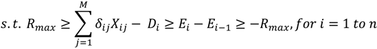
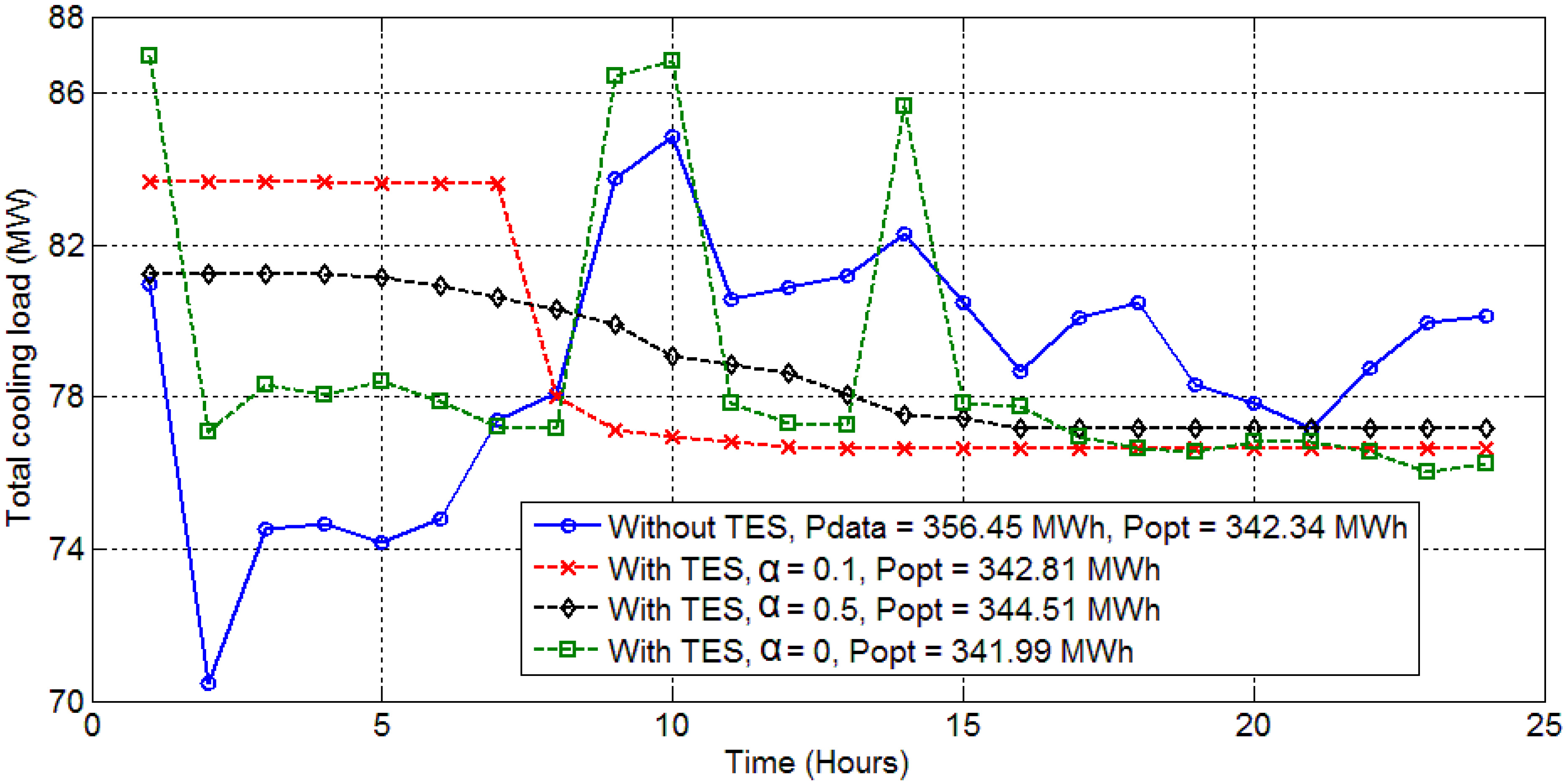
Figure 5 presents the comparison among various distributions of the optimal cooling load from the stage 1 of dynamic optimization,
i.e., the redistribution of cooling load among several hours.
Figure 6 presents similar results for Day 2, which has less frequent cooling load variations as compared to Day 1. For each day, the optimization problem was solved for different values for the penalty coefficient, α = 0, 0.1 and 0.5 $/kW. It is clearly visible from the
Figure 5 and
Figure 6 that the usage of thermal energy storage provides flexibility to shift cooling load across time and hence to opt for alternate cooling load profiles for a chosen time horizon (24 h in this case). This flexibility comes with the opportunities to save energy and/or to reduce fluctuations in the cooling load profile. These figures show various cooling load profiles for different optimization parameters, each profile independently satisfying the hourly cooling demand constraints.
Figure 5.
Cooling load distribution among 24 h (Day 1) from different optimization conditions.
Figure 5.
Cooling load distribution among 24 h (Day 1) from different optimization conditions.
Figure 6.
Cooling load distribution among 24 h (Day 2) from different optimization conditions.
Figure 6.
Cooling load distribution among 24 h (Day 2) from different optimization conditions.
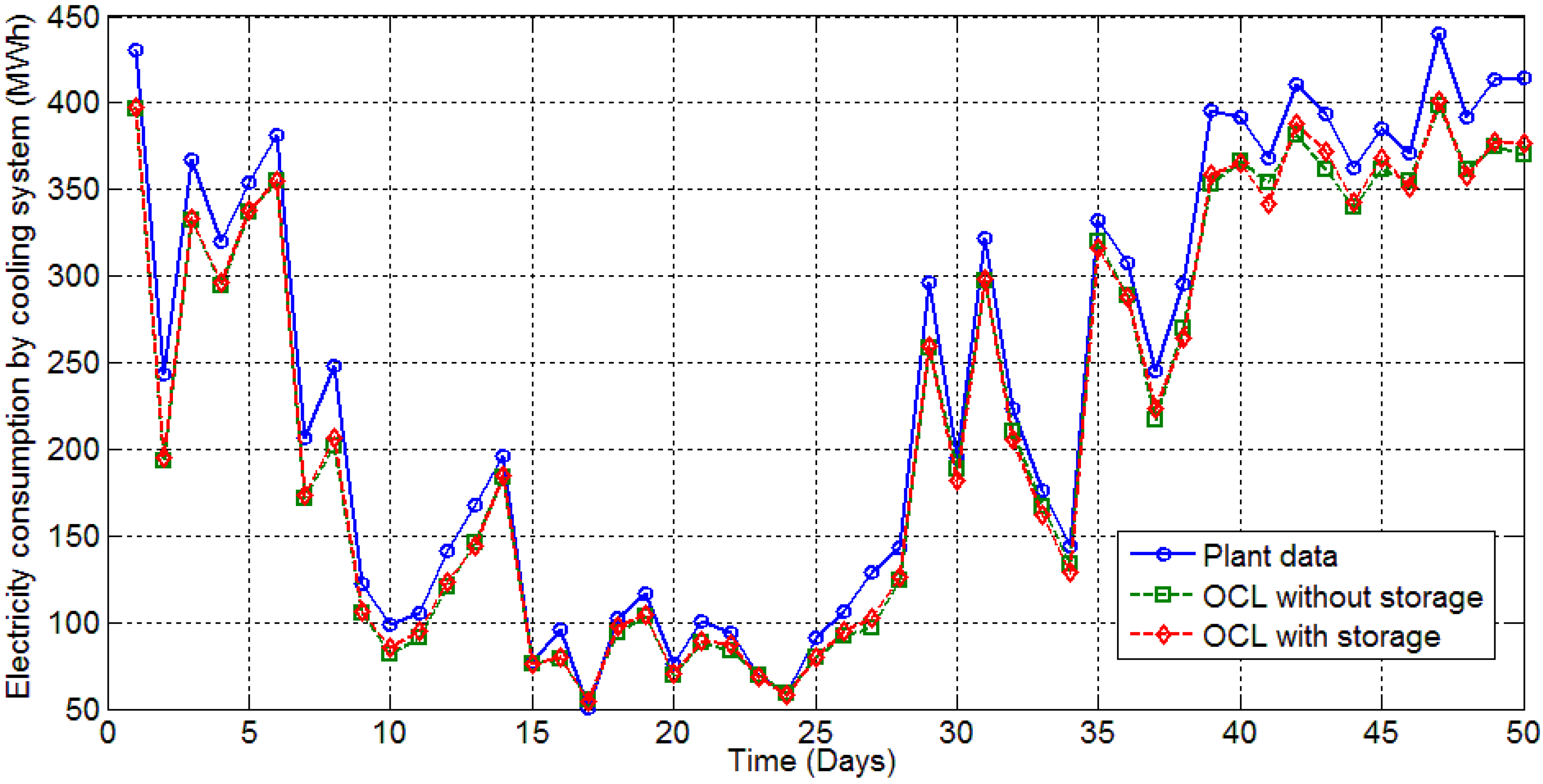
Figure 7 compares the electricity consumption by the overall cooling system, as predicted by the proposed optimization strategies and as gathered from the historical data of the power plant. The comparison is done between the daily cost values of electricity. As a constant electricity price is assumed for this section, the electricity consumption is compared between the plant data and the optimization results with and without storage for a total of 366 data points over a year.
Figure 7 summarizes the results for the year by showing the system’s electricity consumption for 50 representative days over the year.
Figure 7.
Comparison of power consumption values from plant data, static optimization and dynamic optimization.
Figure 7.
Comparison of power consumption values from plant data, static optimization and dynamic optimization.
It can be observed from
Figure 7, that solving OCL with storage does not seem to predict significant energy savings as compared to solving OCL without storage. The results from 366 days of the year 2012 predict a maximum of 6.3% of daily energy savings from using TES as compared to OCL without TES. On an average day, the usage of TES could save about 1.5% of energy consumed by the cooling system. This study does not take into account the heat losses associated with transporting chilled water to and from the storage tank. Hence, in reality the savings are expected to be less than the predictions from the above mentioned optimization study. This is in agreement with other work that has demonstrated minimal energy savings for TES in the Austin, Texas, climate [
14]. As the wet bulb temperature is nearly constant during the summer time (the standard deviation of the wet bulb temperature from June through August is less than 2 °C), there is little opportunity to gain efficiency improvement through the shifting of loads.
However, an interesting observation is made from the above results (
Figure 5 and
Figure 6) about the effect of optimization on the reduced amount of fluctuations of cooling load profile over 24 h. It can be seen qualitatively that as α increases, the optimal use of thermal storage generates a closer to flat cooling load profile for the 24 h at no or negligible extra energy consumption. Therefore as the value of the penalty coefficient α is increased, the resultant optimal cooling load profile would require fewer events of turning chillers on or off. This effect is quantitatively studied for Day 1 (
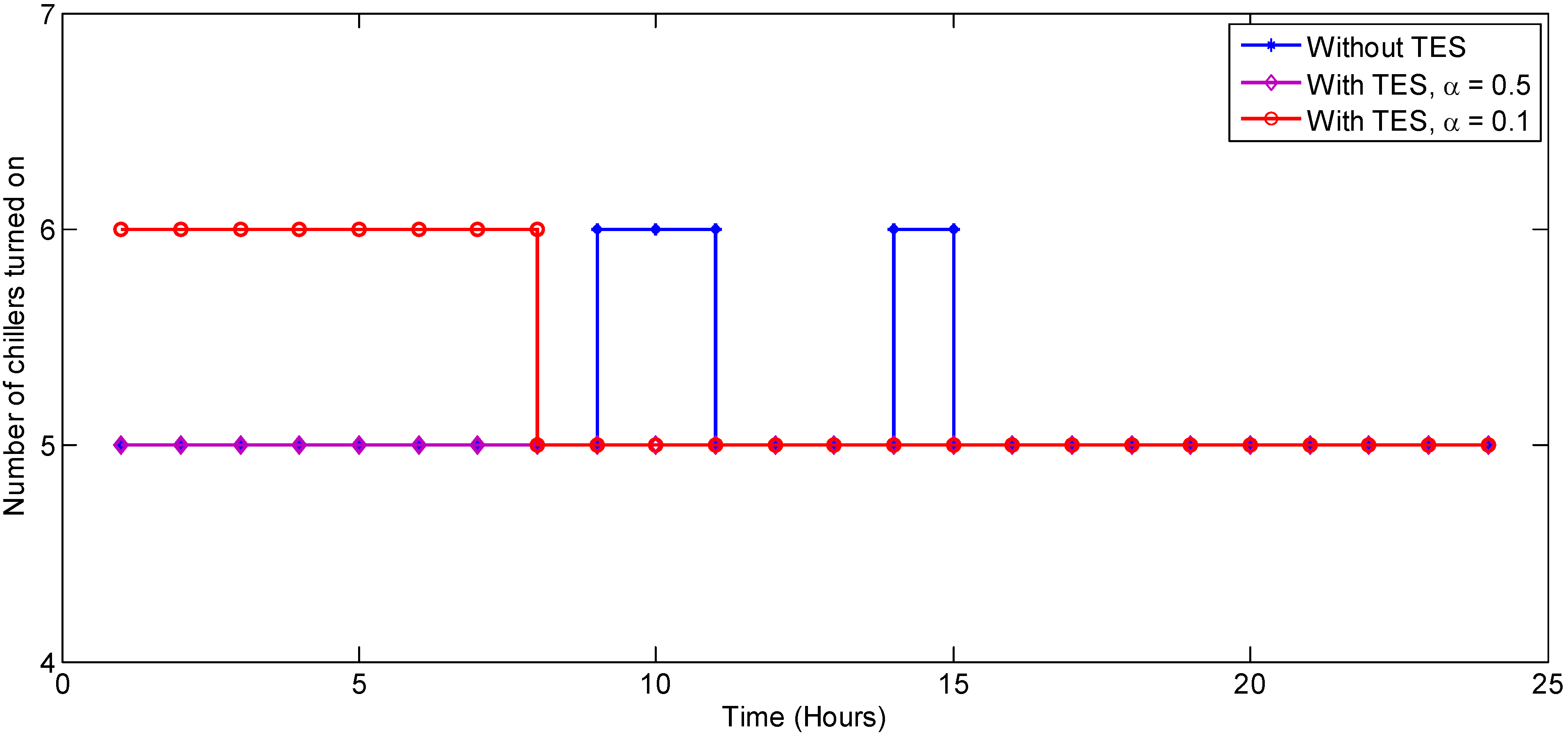
Figure 5). A variable
Ni is defined as the number of chillers operating during the
ith hour. The difference between the values of
Ni for any consecutive hours represents the number of turning on/off events occurring between those two hours. It is assumed that between any two hours, either some chillers are turned on (rise in cooling load) or some chillers are turned off (drop in cooling load) and not both.
Table 4 and
Figure 8 show the results from the abovementioned study for Day 1. The number of times a chiller is turned on or off over a period of 24 h is compared for different cooling load profiles resulting from different optimization parameters,
i.e., the usage of TES and the penalty coefficient α. As α is increased, the penalty cost in the objective function due to the cooling load variation increases. Hence, the optimal cooling load profile seems to be more flat qualitatively and demonstrates less of a need to turn on/off chillers. As the introduction of the penalty coefficient moves the focus of optimization from minimizing the energy consumption, there is a small cost of energy to be paid for a lesser fluctuating cooling load profile. For example, for Day 1, by increasing the value of α from 0 to 0.1, the number of chiller turning on/off events can be reduced from 5 to 1 for a rise in energy consumption as little as 0.24% (
Table 4). It comes out as an interesting trade-off situation where determining an optimal value of α can be another optimization problem.
Table 4.
Effect of optimal chiller loading (OCL) with thermal energy storage on the frequency of cold starts.
Table 4.
Effect of optimal chiller loading (OCL) with thermal energy storage on the frequency of cold starts.
| Cooling load profile | Number of chiller turning on/off events in 24 h | Total power consumption in 24 h (MWh) |
|---|
| Plant data | 4 | 356.45 |
| OCL Without storage | 4 | 342.34 |
| OCL With storage, α = 0 | 5 | 341.99 |
| OCL With storage, α = 0.1 | 1 | 342.81 |
| OCL With storage, α = 0.5 | 0 | 344.51 |
Figure 8.
Comparison of the variations in the total number of operating chillers under different cooling load profiles.
Figure 8.
Comparison of the variations in the total number of operating chillers under different cooling load profiles.
5.1. Time-Varying Prices
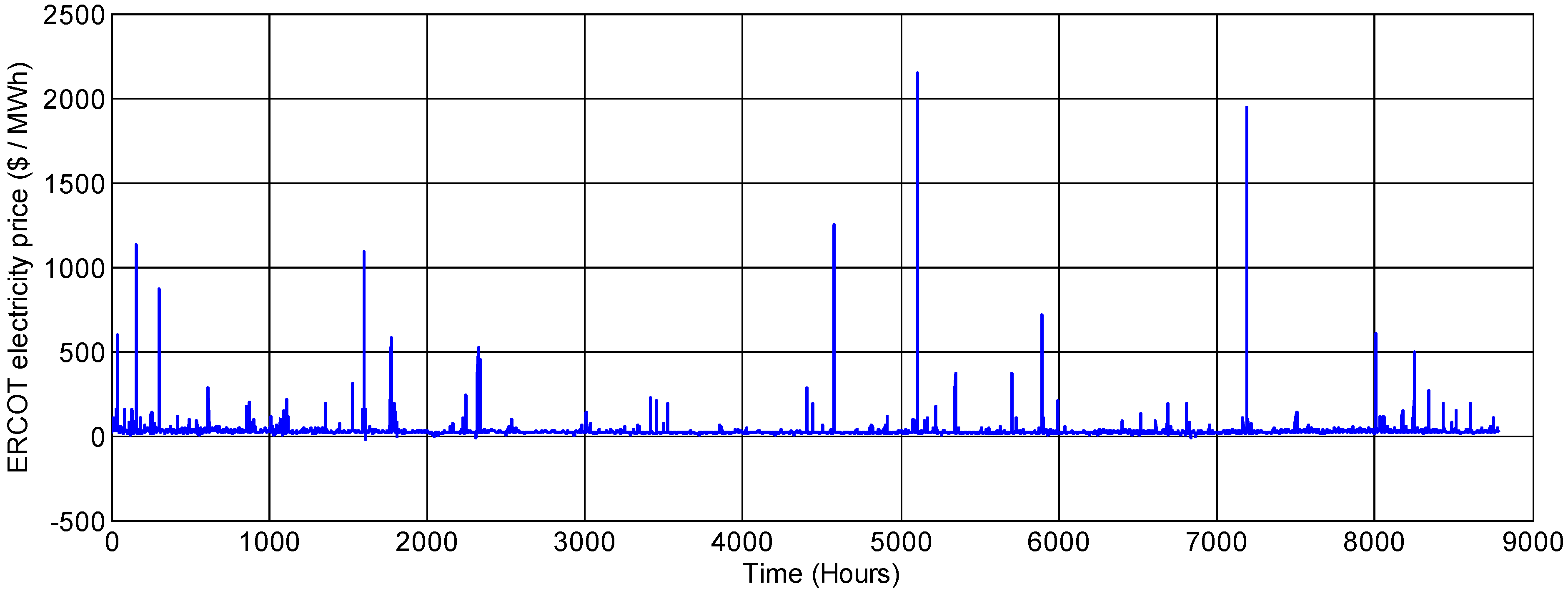
This section evaluates the advantages of using thermal storage in a scenario where electricity prices vary hourly. Real-time market prices from the Austin Load Zone in the Electricity Reliability Council of Texas (ERCOT) market, from 2012, were used for the analysis of optimization results. Such a variable cost scenario highlights the advantage of using thermal energy storage. The market price data (
Figure 9) shows that prices do vary hourly and sometimes quite dramatically,
i.e., by orders of magnitude. A very large cost saving opportunity lies in shifting the cooling load from high cost hours to low cost hours with the help of energy storage.
Figure 9.
Variation in the hourly real-time prices in the ERCOT wholesale market over the year 2012, in Austin, TX, USA.
Figure 9.
Variation in the hourly real-time prices in the ERCOT wholesale market over the year 2012, in Austin, TX, USA.
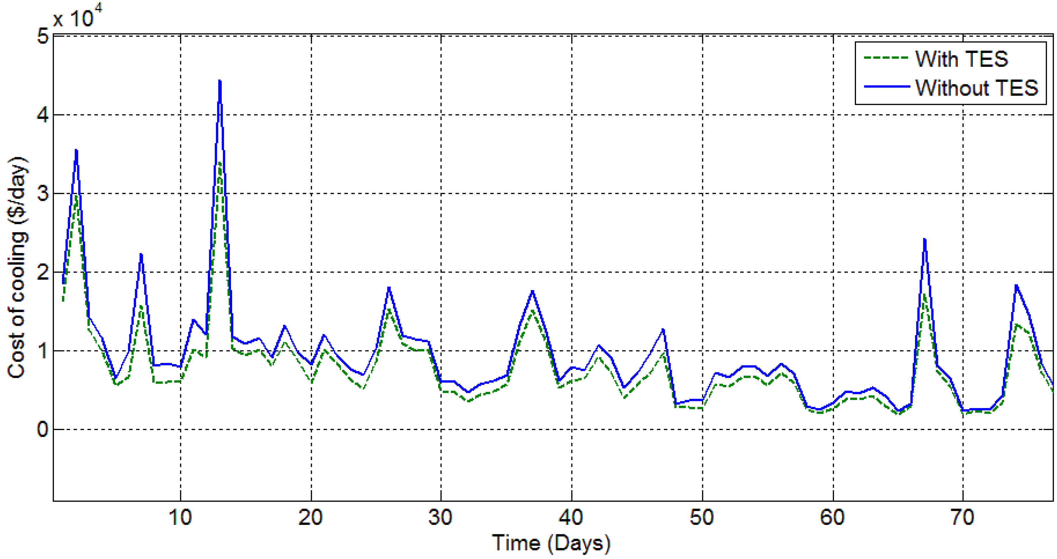
For the purpose of studying the effect of using TES in the case of time varying prices, the value of α was assumed to be zero while solving the optimization problem with storage. Possible savings from using TES in this case were simulated for 366 days of the year 2012 by solving 366 optimization problems. The daily optimal cost (with TES) is compared with the daily estimated cost (without TES) based on real hourly cooling load values and the variable price of electricity from ERCOT. The days with large variation in the electricity price demonstrate large savings in the cost of cooling. The percentage savings in the cooling cost for an hour are predicted to be up to 42.2% with a mean of 13.45%. In an absolute sense, it translates to a sum total of $400,000 saved over a year for a large system such as UT Austin.
Figure 10 shows the comparison between daily cost to cool the campus, with and without using thermal energy storage. For the purpose of clarity, this figure shows the results for only 75 consecutive days from the year 2012. The energy cost savings through the optimal usage of thermal storage is more pronounced in days with high electricity price fluctuation. On a day with high electricity price fluctuations, all or most of its cooling load is spread over hours with low cost and the least amount of chiller operation occurs during the peak cost hours. The excess chilled water generated during the low cost hours is sent to the thermal storage tank. This chilled water is used to satisfy the campus cooling demand during the peak cost hours. Therefore, a significant amount of money can be saved just by using the already existing thermal storage tank in an optimal fashion.
Figure 10.
Comparison of the cooling cost in case of time varying electricity prices—With TES (α = 0) vs. without TES.
Figure 10.
Comparison of the cooling cost in case of time varying electricity prices—With TES (α = 0) vs. without TES.
6. Conclusions
In the current paper, the optimization of a large scale cooling system was performed using various MINLP formulations. The optimization results were compared against the hourly real plant data from UT Austin chiller plants spanning over one year. Multi-period static optimal chiller loading yielded energy savings up to 40% for a time period (one hour). Assuming a constant electricity cost of 6 cents/kWh, annual savings of $486,000 were estimated for the year 2012. Hence, optimal chiller loading emerges as an effective way to reduce electrical energy consumption. As the cooling system at UT Austin consumes over 30% of the annual total power generation, efficient operation of cooling system will reduce the load on power generation equipment.
Addition of thermal energy storage to the cooling system provides additional flexibility in its operation. A multi-period optimization problem over a larger time horizon (24 h) was solved to study the effect of using TES on power consumption and operational stability. The results in this case did not translate to significant energy savings. Moreover, the objective function did not include the heat losses associated with the use of TES. Therefore in a real situation, the energy savings from using TES are expected to be somewhat lower. However, for a hypothetical scenario of time varying electricity prices, shifting of cooling load with the help of TES predicted economic savings up to 42.2% for a day.
The optimal operation of cooling system with TES was also shown to have a significant positive impact on the chiller plant operations in terms of the frequency of cold starts. Due to the added flexibility to adjust the cooling load profile, the cooling system with TES was able to generate a less fluctuating operating strategy with the help of the proposed optimization routine. It was shown that the number of occurrences of turning a chiller on or off over a period of 24 h can be reduced from 4 to 0 by using thermal storage. It is expected to even further reduce the energy losses that occur during the transient phase of a chiller operation. Additionally, with a smoother cooling operation, the equipment wear is also expected to be reduced.
The findings from the current study suggest that optimal chiller loading is an effective energy saving operating strategy for large scale cooling systems with multiple chillers sharing a common cooling load. The installation and operation of thermal energy storage (TES) is marginally beneficial to save energy costs where the cost of electricity is constant with time. On the other hand, the use of TES can minimize the fluctuations in cooling load profile. In situations where time varying electricity prices are used, TES is shown to be quite useful in reducing electricity bills. The current study can be further extended in many ways. The choice of time horizon of the optimization problem with TES can have a significant impact on improving the cooling operation. The starting point of one optimization cycle was assumed to be midnight in the current study, assuming an empty TES tank at that time. Different starting points also need to be considered in order to expand the proposed study. For systems like UT Austin, shifting of cooling loads with the help of TES can also shift loads on the power generation equipment. Variable efficiency curves of turbines suggest another possible optimization problem to minimize the total natural gas consumption by the power plant.

