Selective Wander Join: Fast Progressive Visualizations for Data Joins


Abstract
1. Introduction
- SELECT AVG(orders.order_total), location.region
- FROM orders, customers, location
- WHERE orders.customerID = customer.customerID AND
- customer.locationID = location.locationID
- GROUP BY location.region
- Extended online aggregation methods to support joins for common visualization queries, such as filtering and grouping.
- A method for providing a uniform convergence rate for all GROUP BY categories, regardless of data membership in each group.
- An application of common interaction techniques to view and adjust sampling rates in progressive visualizations.
2. Related Work
2.1. Progressive Visual Analytics
2.2. Data Systems for Interactive Data Exploration
2.3. Online Aggregation, Ripple Join, and Wander Join
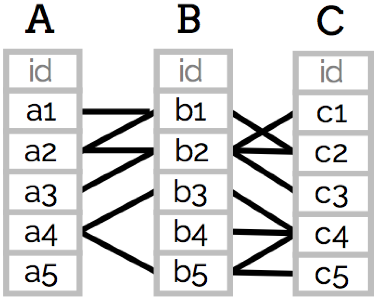
3. Wander Join Algorithm
3.1. Using Wander Join in Visual Exploration
3.1.1. Data
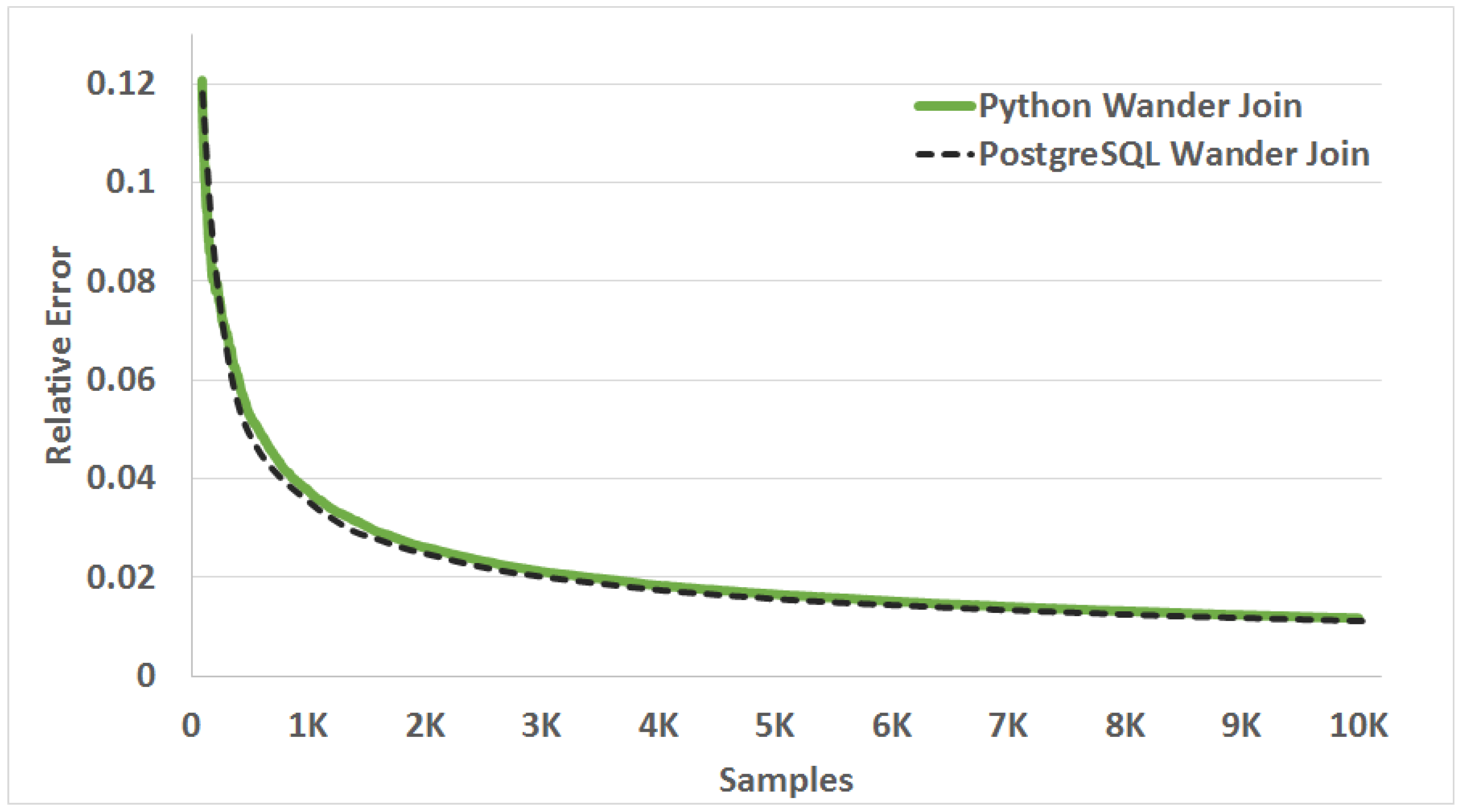
3.1.2. Validation Experiment
- SELECT sum(l_quantity)
- FROM part, lineitem
- WHERE part.p_partkey = lineitem.l_partkey
3.1.3. Evaluating GROUP BY Queries
- SELECT sum(l_quantity)
- FROM part, lineitem
- WHERE part.p_partkey = lineitem.l_partkey
- GROUP BY part.p_size
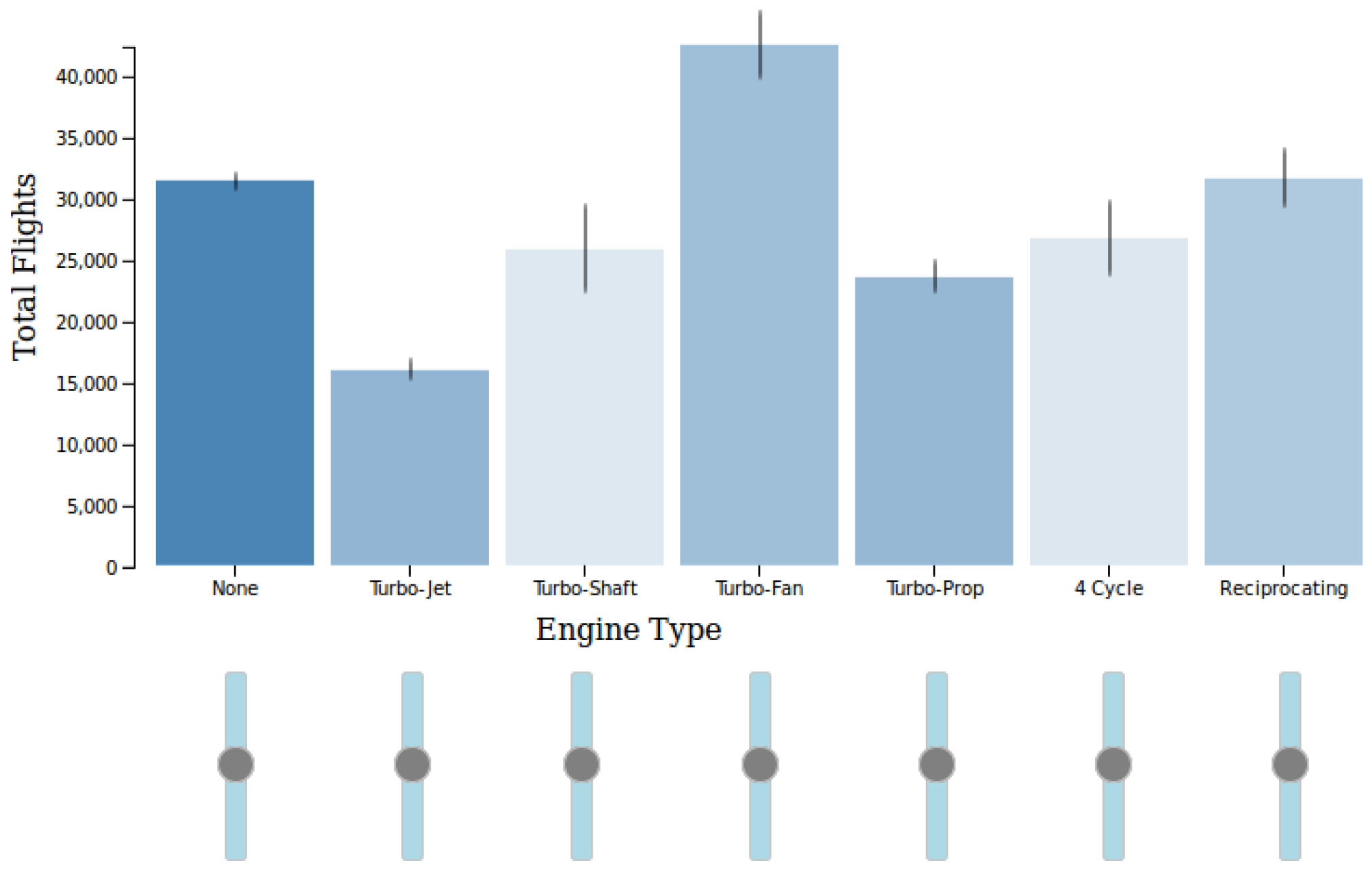
3.1.4. Evaluating Wander Join Using a Real World Dataset
- SELECT count(*)
- FROM plane_data, flights
- WHERE plane_data.tail_num = flights.tail_num
- GROUP BY plane_data.engine_type
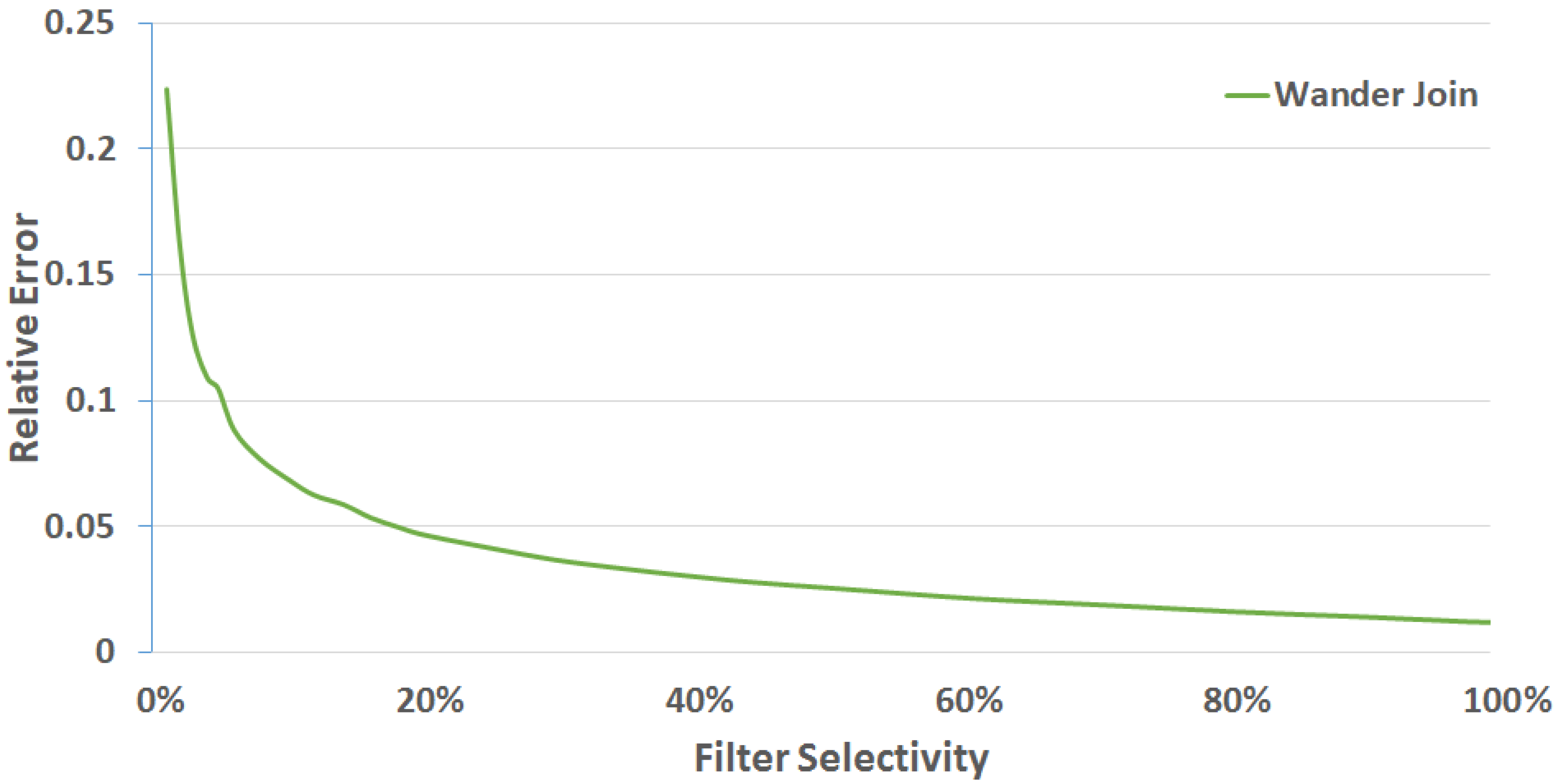
3.1.5. Evaluating Selective Queries
- SELECT sum(l_quantity)
- FROM part, lineitem
- WHERE part.p_partkey = lineitem.l_partkey
- AND part.p_size <= X
- AND lineitem.l_quantity <= Y
4. Limitations of Wander Join
5. Selective Wander Join: Wander Join for Visual Data Exploration
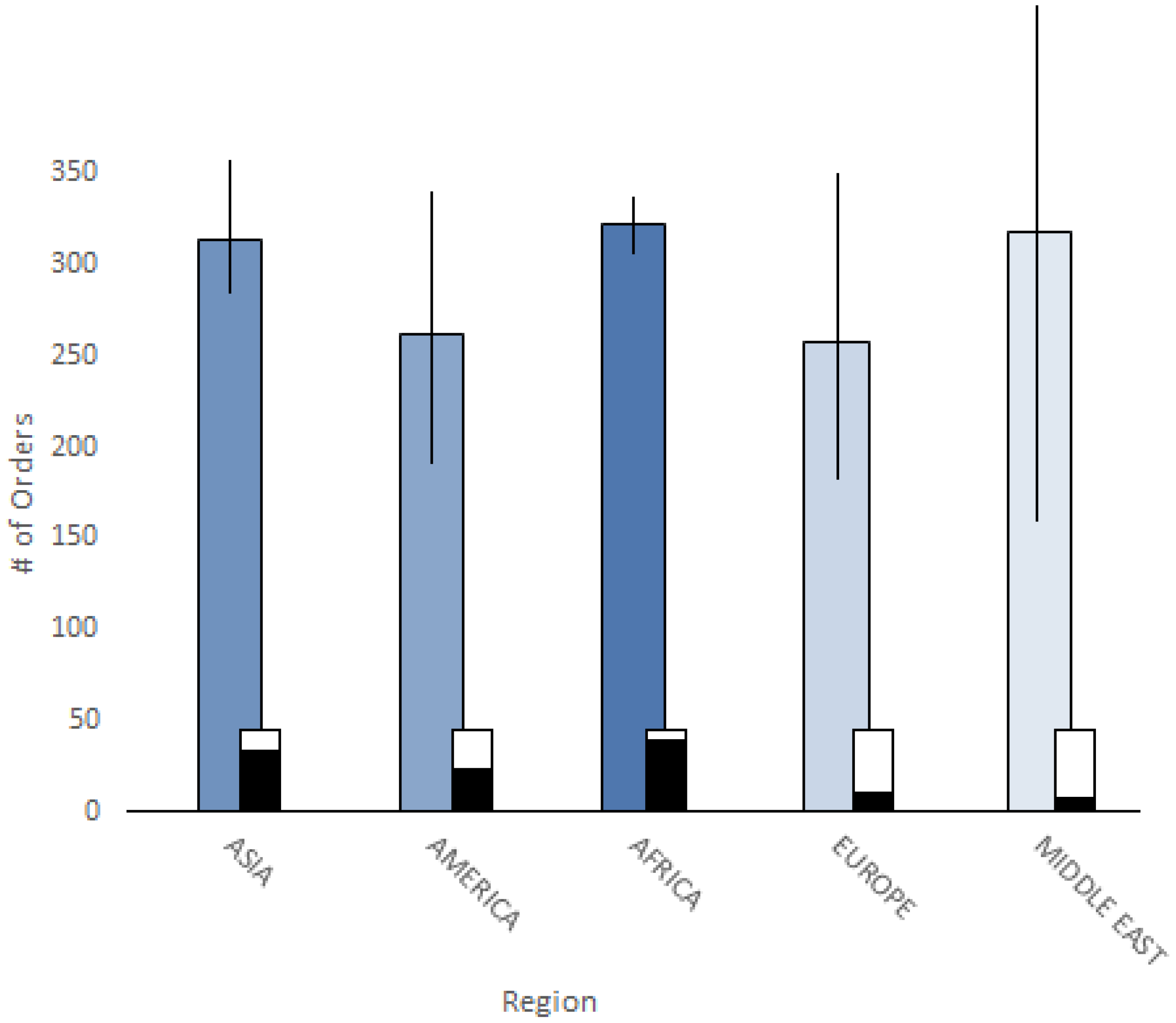
5.1. Optimizing for Group By Queries
5.1.1. Method
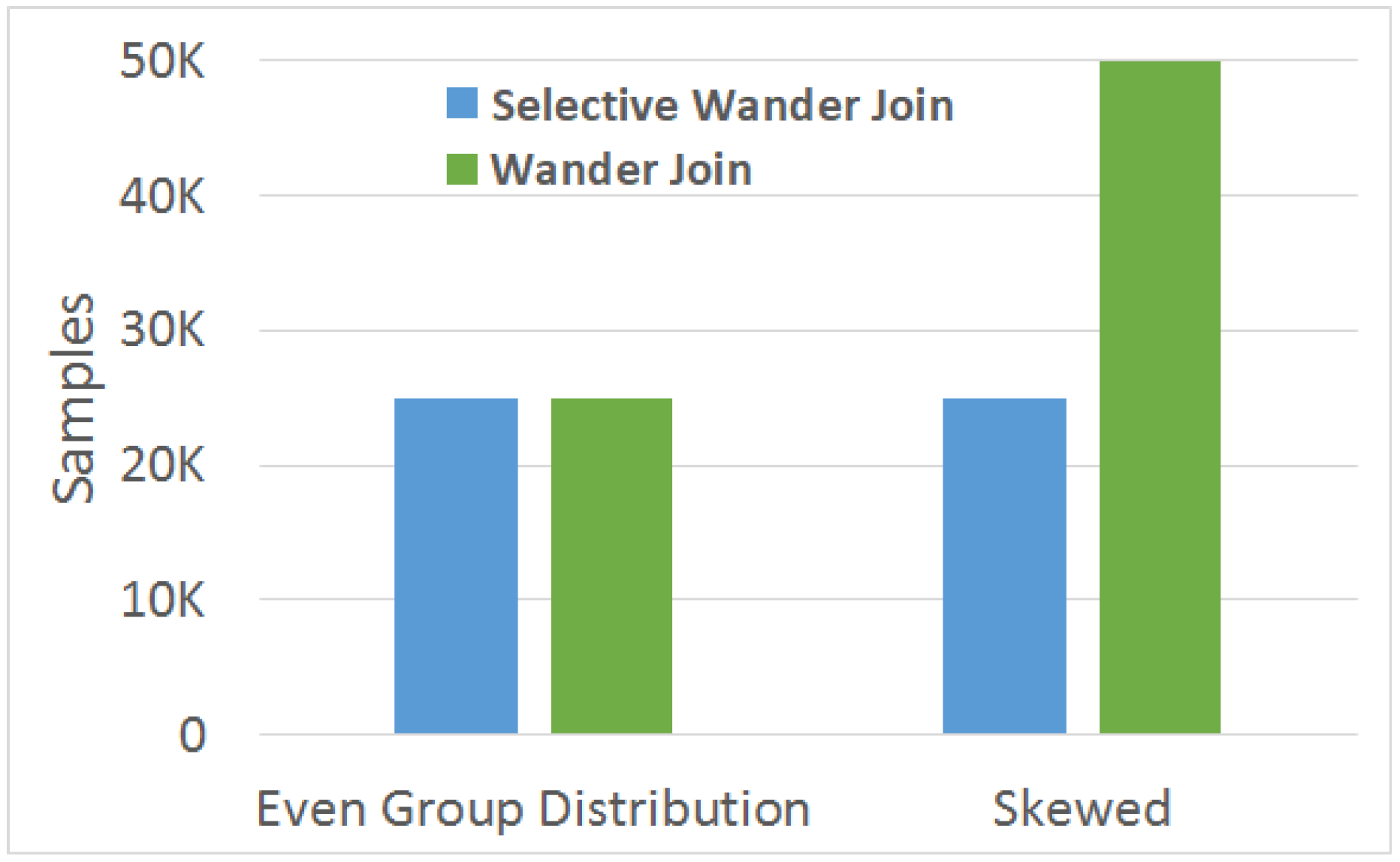
5.1.2. Evaluation
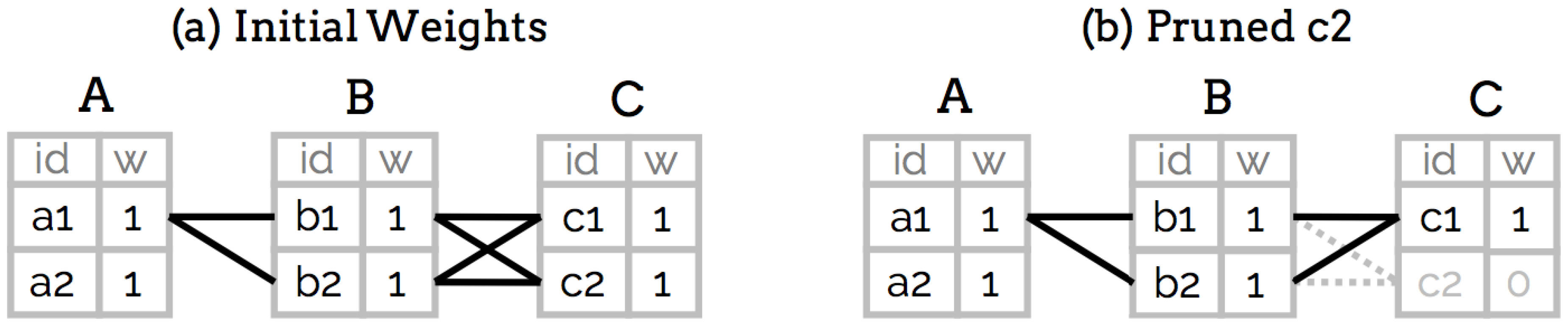
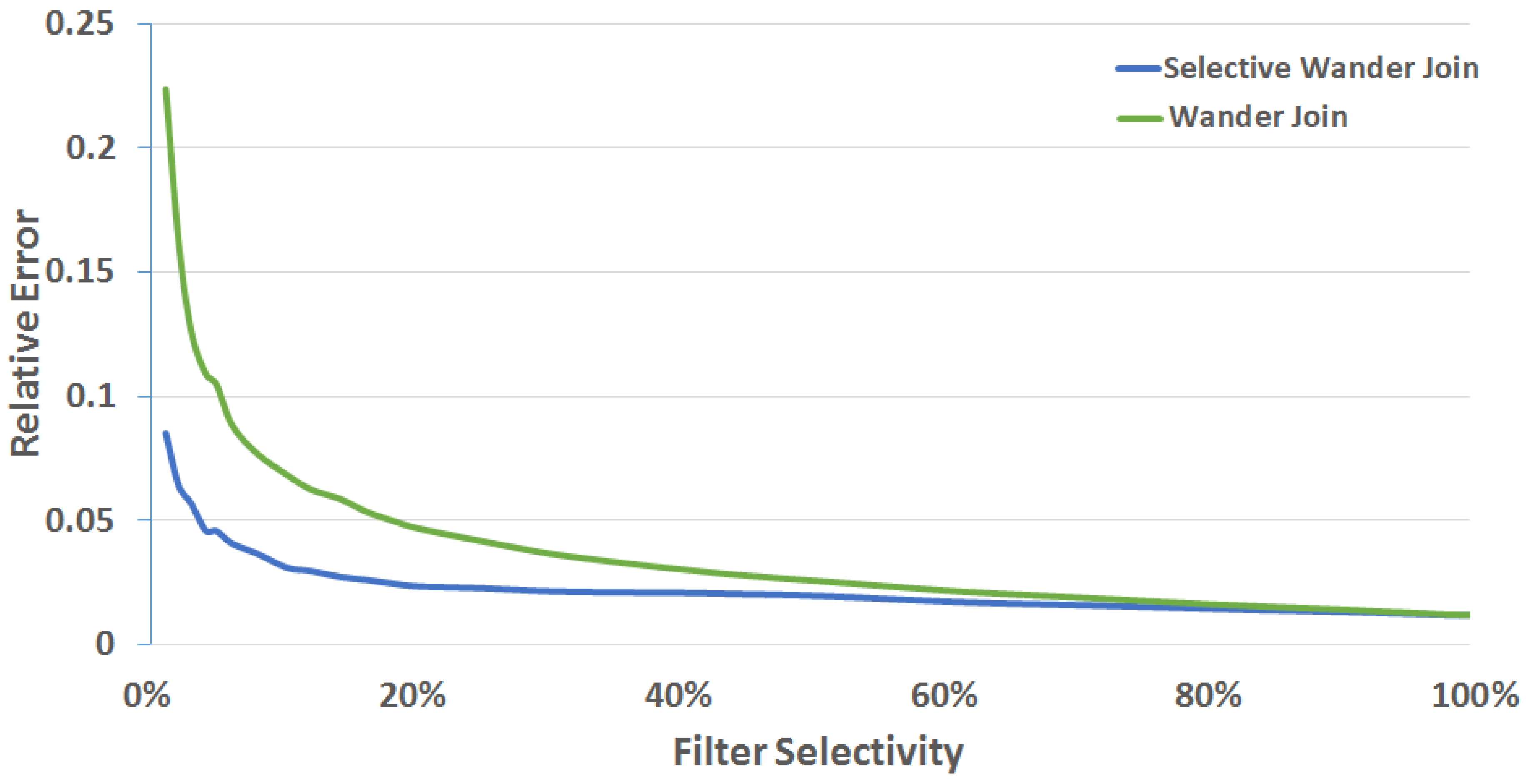
5.2. Optimizing for Highly Selective Queries
5.2.1. Method
5.2.2. Evaluation
- SELECT sum(l_quantity)
- FROM part, lineitem
- WHERE part.p_partkey = lineitem.l_partkey
- AND part.p_size <= X
- AND lineitem.l_quantity <= Y
5.2.3. Extensions
5.3. Trading Complexity for Usability
6. User-Driven Sampling in Selective Wander Join
7. Expert User Study
7.1. Study Setup
7.2. Results
7.2.1. Task 1 Results
7.2.2. Task 2 Results
7.3. Discussion
7.3.1. Efficacy of the Selective Wander Join Visual Interface
7.3.2. Weight Adjustments
7.3.3. Timing of Weight Adjustments
8. Conclusions
Author Contributions
Funding
Conflicts of Interest
References
- Selinger, P.G.; Astrahan, M.M.; Chamberlin, D.D.; Lorie, R.A.; Price, T.G. Access path selection in a relational database management system. In Proceedings of the 1979 ACM SIGMOD international conference on Management of data, Boston, MA, USA, 30 May–1 June 1979; pp. 23–34. [Google Scholar]
- Hastings, W.K. Monte Carlo sampling methods using Markov chains and their applications. Biometrika 1970, 57, 97–109. [Google Scholar] [CrossRef]
- Li, F.; Wu, B.; Yi, K.; Zhao, Z. Wander Join: Online Aggregation via Random Walks. In Proceedings of the 2016 International Conference on Management of Data, San Francisco, CA, USA, 26 June–1 July 2016; pp. 615–629. [Google Scholar]
- Wu, E.; Battle, L.; Madden, S.R. The case for data visualization management systems: Vision paper. Proc. VLDB Endow. 2014, 7, 903–906. [Google Scholar] [CrossRef]
- Wu, E.; Psallidas, F.; Miao, Z.; Zhang, H.; Rettig, L.; Wu, Y.; Sellam, T. Combining Design and Performance in a Data Visualization Management System. In Proceedings of the Conference on Innovative Data Systems Research, Chaminade, CA, USA, 8–11 January 2017. [Google Scholar]
- Mühlbacher, T.; Piringer, H.; Gratzl, S.; Sedlmair, M.; Streit, M. Opening the black box: Strategies for increased user involvement in existing algorithm implementations. IEEE Trans. Vis. Comput. Graph. 2014, 20, 1643–1652. [Google Scholar] [CrossRef] [PubMed]
- Angelini, M.; Santucci, G.; Schumann, H.; Schulz, H.J. A Review and Characterization of Progressive Visual Analytics. Inform. Multidiscip. Dig. Publ. Inst. 2018, 5, 31. [Google Scholar] [CrossRef]
- Stolper, C.D.; Perer, A.; Gotz, D. Progressive visual analytics: User-driven visual exploration of in-progress analytics. IEEE Trans. Vis. Comput. Graph. 2014, 20, 1653–1662. [Google Scholar] [CrossRef] [PubMed]
- Pezzotti, N.; Lelieveldt, B.; van der Maaten, L.; Hollt, T.; Eisemann, E.; Vilanova, A. Approximated and user steerable tsne for progressive visual analytics. IEEE Trans. Vis. Comput. Graph. 2016, 23, 1739–1752. [Google Scholar] [CrossRef] [PubMed]
- Turkay, C.; Kaya, E.; Balcisoy, S.; Hauser, H. Designing Progressive and Interactive Analytics Processes for High-Dimensional Data Analysis. IEEE Trans. Vis. Comput. Graph. 2017, 23, 131–140. [Google Scholar] [CrossRef] [PubMed]
- Fisher, D.; Popov, I.; Drucker, S. Trust me, I’m partially right: Incremental visualization lets analysts explore large datasets faster. In Proceedings of the SIGCHI Conference on Human Factors in Computing Systems, Austin, TX, USA, 5–10 May 2012; pp. 1673–1682. [Google Scholar]
- Fisher, D. Incremental, approximate database queries and uncertainty for exploratory visualization. In Proceedings of the 2011 IEEE Symposium on Large Data Analysis and Visualization (LDAV), Providence, RI, USA, 23–24 October 2011; pp. 73–80. [Google Scholar]
- Hellerstein, J.M.; Avnur, R.; Chou, A.; Hidber, C.; Olston, C.; Raman, V.; Roth, T.; Haas, P.J. Interactive data analysis: The control project. Computer 1999, 32, 51–59. [Google Scholar] [CrossRef]
- Zgraggen, E.; Galakatos, A.; Crotty, A.; Fekete, J.D.; Kraska, T. How Progressive Visualizations Affect Exploratory Analysis. IEEE Trans. Vis. Comput. Graph. 2016, 23, 1977–1987. [Google Scholar] [CrossRef] [PubMed]
- Moritz, D.; Fisher, D.; Ding, B.; Wang, C. Trust, but Verify: Optimistic Visualizations of Approximate Queries for Exploring Big Data. In Proceedings of the 2017 CHI Conference on Human Factors in Computing Systems, Denver, CO, USA, 6–11 May 2017. [Google Scholar]
- Fekete, J.D. Progressivis: A toolkit for steerable progressive analytics and visualization. In Proceedings of the 1st Workshop on Data Systems for Interactive Analysis, Chicago, IL, USA, 17–21 October 2015; p. 5. [Google Scholar]
- Rosenbaum, R.; Schumann, H. Progressive refinement: More than a means to overcome limited bandwidth. In Proceedings of the IS&T/SPIE Electronic Imaging, San Jose, CA, USA, 24 January 2009; p. 72430I. [Google Scholar]
- Badam, S.K.; Elmqvist, N.; Fekete, J.D. Steering the craft: UI elements and visualizations for supporting progressive visual analytics. In Computer Graphics Forum; Wiley Online Library: Hoboken, NJ, USA, 2017; Volume 36, pp. 491–502. [Google Scholar]
- Stolte, C.; Tang, D.; Hanrahan, P. Polaris: A system for query, analysis, and visualization of multidimensional relational databases. IEEE Trans. Vis. Comput. Graph. 2002, 8, 52–65. [Google Scholar] [CrossRef]
- Lins, L.; Klosowski, J.T.; Scheidegger, C. Nanocubes for real-time exploration of spatiotemporal datasets. IEEE Trans. Vis. Comput. Graph. 2013, 19, 2456–2465. [Google Scholar] [CrossRef] [PubMed]
- Liu, Z.; Jiang, B.; Heer, J. imMens: Real-time Visual Querying of Big Data. In Computer Graphics Forum; Wiley Online Library: Hoboken, NJ, USA, 2013; Volume 32, pp. 421–430. [Google Scholar]
- Pahins, C.A.; Stephens, S.A.; Scheidegger, C.; Comba, J.L. Hashedcubes: Simple, low memory, real-time visual exploration of big data. IEEE Trans. Vis. Comput. Graph. 2017, 23, 671–680. [Google Scholar] [CrossRef] [PubMed]
- Wang, Z.; Ferreira, N.; Wei, Y.; Bhaskar, A.S.; Scheidegger, C. Gaussian Cubes: Real-Time Modeling for Visual Exploration of Large Multidimensional Datasets. IEEE Trans. Vis. Comput. Graph. 2017, 23, 681–690. [Google Scholar] [CrossRef] [PubMed]
- Agarwal, S.; Mozafari, B.; Panda, A.; Milner, H.; Madden, S.; Stoica, I. BlinkDB: Queries with bounded errors and bounded response times on very large data. In Proceedings of the 8th ACM European Conference on Computer Systems, Prague, Czech Republic, 15–17 April 2013; pp. 29–42. [Google Scholar]
- Ding, B.; Huang, S.; Chaudhuri, S.; Chakrabarti, K.; Wang, C. Sample+ Seek: Approximating Aggregates with Distribution Precision Guarantee. In Proceedings of the 2016 International Conference on Management of Data, San Francisco, CA, USA, 26 June–1 July 2016; pp. 679–694. [Google Scholar]
- Kamat, N.; Jayachandran, P.; Tunga, K.; Nandi, A. Distributed and interactive cube exploration. In Proceedings of the 2014 IEEE 30th International Conference on Data Engineering (ICDE), Chicago, IL, USA, 31 March–4 April 2014; pp. 472–483. [Google Scholar]
- Li, X.; Han, J.; Yin, Z.; Lee, J.G.; Sun, Y. Sampling cube: A framework for statistical olap over sampling data. In Proceedings of the 2008 ACM SIGMOD international conference on Management of data, Vancouver, BC, Canada, 10–12 June 2008; pp. 779–790. [Google Scholar]
- Fekete, J.D.; Primet, R. Progressive analytics: A computation paradigm for exploratory data analysis. arXiv, 2016; arXiv:1607.05162. [Google Scholar]
- Im, J.F.; Villegas, F.G.; McGuffin, M.J. Visreduce: Fast and responsive incremental information visualization of large datasets. In Proceedings of the 2013 IEEE International Conference on Big Data, Santa Clara, CA, USA, 6–9 October 2013; pp. 25–32. [Google Scholar]
- Chaudhuri, S.; Das, G.; Narasayya, V. Optimized stratified sampling for approximate query processing. ACM Trans. Database Syst. 2007, 32, 9. [Google Scholar] [CrossRef]
- Park, Y.; Cafarella, M.; Mozafari, B. Visualization-aware sampling for very large databases. In Proceedings of the 2016 IEEE 32nd International Conference on Data Engineering (ICDE), Helsinki, Finland, 16–20 May 2016; pp. 755–766. [Google Scholar]
- Doshi, P.R.; Geraldine, E.; Rosario, G.; Rundensteiner, E.; Ward, M. A strategy selection framework for adaptive prefetching in data visualization. In Proceedings of the 15th International Conference on Scientific and Statistical Database Management, Cambridge, MA, USA, 9–11 July 2003; pp. 107–116. [Google Scholar]
- Chan, S.M.; Xiao, L.; Gerth, J.; Hanrahan, P. Maintaining interactivity while exploring massive time series. In Proceedings of the IEEE Symposium on Visual Analytics Science and Technology, Columbus, OH, USA, 19–24 October 2008; pp. 59–66. [Google Scholar]
- Battle, L.; Chang, R.; Stonebraker, M. Dynamic prefetching of data tiles for interactive visualization. In Proceedings of the 2016 International Conference on Management of Data, San Francisco, CA, USA, 26 June–1 July 2016; pp. 1363–1375. [Google Scholar]
- Cetintemel, U.; Cherniack, M.; DeBrabant, J.; Diao, Y.; Dimitriadou, K.; Kalinin, A.; Papaemmanouil, O.; Zdonik, S.B. Query Steering for Interactive Data Exploration. In Proceedings of the Conference on Innovative Data Systems Research (CIDR), Asilomar, CA, USA, 6–9 January 2013. [Google Scholar]
- Stonebraker, M.; Abadi, D.J.; Batkin, A.; Chen, X.; Cherniack, M.; Ferreira, M.; Lau, E.; Lin, A.; Madden, S.; O’Neil, E.; et al. C-store: A column-oriented DBMS. In Proceedings of the 31st International Conference on Very Large Data Bases, Trondheim, Norway, 30 August–2 September 2005; pp. 553–564. [Google Scholar]
- Kemper, A.; Neumann, T. HyPer: A hybrid OLTP&OLAP main memory database system based on virtual memory snapshots. In Proceedings of the 2011 IEEE 27th International Conference on Data Engineering (ICDE), Hannover, Germany, 11–16 April 2011; pp. 195–206. [Google Scholar]
- Godfrey, P.; Gryz, J.; Lasek, P. Interactive visualization of large data sets. IEEE Trans. Knowl. Data Eng. 2016, 28, 2142–2157. [Google Scholar] [CrossRef]
- Hellerstein, J.M.; Haas, P.J.; Wang, H.J. Online aggregation. ACM SIGMOD Rec. 1997, 26, 171–182. [Google Scholar] [CrossRef]
- Haas, P.J.; Hellerstein, J.M. Ripple joins for online aggregation. ACM SIGMOD Rec. 1999, 28, 287–298. [Google Scholar] [CrossRef]
- Wickham, H. ASA 2009 Data Expo. J. Comput. Graph. Stat. 2011, 20, 281–283. [Google Scholar] [CrossRef]
- Shneiderman, B. The eyes have it: A task by data type taxonomy for information visualizations. In Proceedings of the IEEE Symposium on Visual Languages, Boulder, CO, USA, 3–6 September 1996; pp. 336–343. [Google Scholar]
- Alabi, D.; Wu, E. PFunk-H: Approximate query processing using perceptual models. In Proceedings of the Workshop on Human-In-the-Loop Data Analytics, San Francisco, CA, USA, 26 June–1 July 2016; p. 10. [Google Scholar]
- Wu, E.; Nandi, A. Towards Perception-aware Interactive Data Visualization Systems. In Proceedings of the DSIA Workshop, Chicago, IL, USA, 26 October 2015. [Google Scholar]


| Relative Error | Selective Wander Join | Wander Join | Sample Ratio |
|---|---|---|---|
| 0.05 | 9982 | 977,432 | 1.021% |
| 0.06 | 3928 | 579,110 | 0.678% |
| 0.07 | 3010 | 439,061 | 0.685% |
| 0.08 | 1836 | 321,732 | 0.571% |
| 0.09 | 1725 | 238,492 | 0.723% |
| 0.10 | 1351 | 221,116 | 0.611% |
| Table Size (Rows) | Filter Query | Group By Query (First Table) |
|---|---|---|
| 10 k | 40 kB | 80 kB |
| 100 k | 400 kB | 800 kB |
| 1 M | 4 MB | 8 MB |
| 10 M | 40 MB | 80 MB |
| 100 M | 400 MB | 800 MB |
| 1 B | 4 GB | 8 GB |
© 2019 by the authors. Licensee MDPI, Basel, Switzerland. This article is an open access article distributed under the terms and conditions of the Creative Commons Attribution (CC BY) license (http://creativecommons.org/licenses/by/4.0/).
Share and Cite
Procopio, M.; Scheidegger, C.; Wu, E.; Chang, R. Selective Wander Join: Fast Progressive Visualizations for Data Joins. Informatics 2019, 6, 14. https://doi.org/10.3390/informatics6010014
Procopio M, Scheidegger C, Wu E, Chang R. Selective Wander Join: Fast Progressive Visualizations for Data Joins. Informatics. 2019; 6(1):14. https://doi.org/10.3390/informatics6010014
Chicago/Turabian StyleProcopio, Marianne, Carlos Scheidegger, Eugene Wu, and Remco Chang. 2019. "Selective Wander Join: Fast Progressive Visualizations for Data Joins" Informatics 6, no. 1: 14. https://doi.org/10.3390/informatics6010014
APA StyleProcopio, M., Scheidegger, C., Wu, E., & Chang, R. (2019). Selective Wander Join: Fast Progressive Visualizations for Data Joins. Informatics, 6(1), 14. https://doi.org/10.3390/informatics6010014