Surrender Risk in the Context of the Quantitative Assessment of Participating Life Insurance Contracts under Solvency II

ifa (Institute for Finance and Actuarial Sciences), Lise-Meitner-Strasse 14, 89081 Ulm, Germany
Risks 2018, 6(3), 66; https://doi.org/10.3390/risks6030066
Submission received: 18 May 2018
/
Revised: 22 June 2018
/
Accepted: 22 June 2018
/
Published: 27 June 2018
(This article belongs to the Special Issue Capital Requirement Evaluation under Solvency II framework)
Abstract
:Participating life insurance contracts entitle the policyholder to participate in the company’s annual surplus. Typically, they are also equipped with a surrender option that allows the policyholder to terminate the contract prior to maturity, receiving a predetermined surrender value. The option interacts with (often cliquet-style) interest guarantees that are a key feature of traditional participating contracts. Surrender options can considerably affect an insurer’s liabilities and bear material risks. This paper addresses the recognition of those risks in the quantitative assessment of a heterogeneous insurance portfolio under Solvency II, taking into account the complex interrelation between minimum interest guarantees, reserving requirements, and profit sharing. The lapse risk module of the Solvency II standard formula requires the identification of portfolio segments that are exposed to a specific change of surrender rates (long-term increase/decrease, one-off increase). We provide a heuristic that identifies homogeneous risk groups in the sense that the respective stress would increase the insurer’s liabilities. Our approach can be used to derive an appropriate segmentation in practical applications. We further analyze implications of the segmentation on the Risk Margin (as part of the Technical Provisions under Solvency II) and discuss consequences of policyholder options on the calculation of Going Concern Reserve and Surplus Funds. To illustrate our findings, we set up a stochastic balance sheet and cash flow projection model for a stylized life insurance company. We conclude that current methods used for practical applications underestimate surrender risk under Solvency II and that the proposed modeling refinements may improve the appropriateness of solvency ratios for participating business.
1. Introduction
Life insurance policies often come with several policyholder options. In particular, this includes the surrender option which allows the policyholder to terminate the contract prior to maturity in combination with the payout of a (predetermined) surrender value. Hence, surrender options may significantly affect a company’s future cash flow profile and have material impact on the insurer’s liabilities (Bauer et al. 2006; Gatzert 2009; Kling et al. 2014).
This especially holds for traditional participating life insurance business, which makes up for a significant part of the life insurance market in Germany (and other member states of the European Union). Such contracts are characterized by two key features: First, they come with an (often cliquet-style) minimum interest guarantee (that may differ within the insurance portfolio). In addition, they are entitled to an appropriate participation in the company’s annual (positive) surplus. In fact, a substantial part of an insurer’s future obligations against policyholders is related to future surplus participation.
The surplus participation process itself is highly complex and results in interaction effects within the insurance portfolio (Burkhart et al. 2015). Policyholders’ surplus participation is not determined on a single contract basis, but the annual surplus is jointly determined for the whole portfolio and allocated to individual contracts in a multi-stage process. The process includes a collective bonus reserve, the so-called Reserve for Bonuses and Rebates (RfB, Rückstellung für Beitragsrückerstattung), in which surplus is pooled first to buffer fluctuations in the annual surplus to achieve a stable surplus participation for all policyholders. As a result, the insurer’s future obligations arising from a specific contract cannot be isolated from the remaining portfolio, but they depend on the guarantees and the development of the entire portfolio.
Due to these interdependencies, the impact of a policyholder exercising her surrender option is not limited to her own contract, but it affects the insurer’s total obligations. In fact, the profit sharing mechanisms lead to diverse interrelations between surrender options, different levels and types of minimum interest guarantees, and policyholders’ surplus participation within a heterogeneous insurance portfolio.
Surrender options also bear material risks for a life insurance company (Kuo et al. 2003): Massive surrenders may cause liquidity issues and force the selling of assets. Surrenders may further lead to a loss of potential future profits. In case of early surrenders, the insurer may not be able to refinance high up-front investments made in the course of acquiring new business. The option can add to adverse selection, reducing the effectiveness of risk diversification and balancing over time. High surrender rates can also have a negative effect on the insurer’s reputation, which may result in even more policyholders surrendering or harm new business. On the other side, low surrender rates bear the risk that the insurer may not be able to meet the obligations resulting from high guarantees given in the past. Clearly, the risks due to a policyholder’s surrender option depend on the contract and in particular, on the contractual minimum interest guarantee.
The high economic relevance of surrender options has drawn the attention not only of academics but also of the industry and regulators, especially in connection with the introduction of increasingly sophisticated financial reporting standards and risk-based solvency requirements such as Solvency II. The latter is the risk-based solvency system that applies to insurance companies in the European Union.
Various authors have done work on the valuation of surrender options. They find that surrender options can be quite valuable (e.g., Albizzati and Geman 1994; Bacinello 2003; Grosen and Jørgensen 2000). Another branch of the existing literature studies the determinants and modeling of surrender behavior, with partly contradictory results.1 e.g., Geneva Association (2012) do so concentrating on potential illiquidity risks in the life insurance sector due to an increase of surrender rates. Surrender risks are also addressed by other authors. In a recent study, Feodoria and Förstemann (2015) stressed the potential risk of a “policyholder run” in case of a sharp increase of interest rates. Similarly, Berdin et al. (2017) examine the impact of rising interest rates in combination with the potential increase of lapse rates on the insurer’s liquidity and solvency. In fact, regulators have identified lapse risk as the most important risk among the life underwriting risks (EIOPA 2011). Lapse risk under Solvency II reflects all risks due to changes in the level or volatility of option exercise rates. Hence, it appears particularly important for an insurer to appropriately assess the surrender risks he is exposed to.
In this paper, we analyze the recognition of surrender risk in the quantitative assessment under Solvency II. The Solvency II standard formula recognizes surrender risk in its lapse risk module. The module includes three different stress scenarios: an immediate mass lapse event as well as a permanent increase and decrease of the expected lapse rates. It requires the identification of portfolio segments that are exposed to a specific event in the sense that the respective stress would increase the insurer’s liabilities. We provide a heuristic that can be used to derive an appropriate segmentation in practical applications. We further compare this heuristic with the segmentation approach currently used by most insurance companies in Germany. For this purpose, we set up a stochastic balance sheet and cash flow projection model for a stylized life insurance company. The model covers the relevant features of the German market, considering statutory requirements as well as typical management rules.
We further discuss surrender risk in the context of the Risk Margin (RM) which is an important part of the Technical Provisions (TP) under Solvency II. To analyze the surrender risk profile of the insurance company, we explicitly project the Solvency Capital Requirement (SCR) for lapse risk over the lifetime of the insurance portfolio. Based on that projection, different methods to approximate the risk profile are compared to an alternative approximation method introduced in this paper. In particular, our comparison includes the method currently applied in the German standard valuation model for Solvency II, developed by the German Insurance Association (GDV 2017a).
Finally, we extend our analysis to the potential impact of a lapse stress on the mechanisms inherent in the German life insurance business that result in two special Basic Own Funds (BOF) items: Going Concern Reserve (GCR) and Surplus Funds (SF). Regarding the former, we study how inheritance effects between the business in-force and expected future new business change in a lapse stress and how this affects the GCR. Regarding the latter, we discuss the impact of a lapse stress on the economic value of SF. We particularly focus on the risk reducing capacity of collective bonus reserves available at the valuation date, which is the basis for the calculation of SF.
The remainder of this paper is organized as follows. Section 2 covers the requirements of Solvency II relevant for subsequent analyses regarding surrender risk. Section 3 introduces the valuation framework underlying the analysis. The results of our analysis are presented and discussed in Section 4. Section 5 summarizes our findings and concludes.
2. Regulatory Requirements on the Recognition of Policyholder Behavior
The following section provides aspects of the Solvency II framework relevant for subsequent analyses. We further discuss regulatory requirements regarding the reflection of policyholder behavior (risk) for the calculation of solvency capital requirements. In particular, we rely on the Solvency II Directive (European Union 2009) and the latest version of the Solvency II Delegated Act (European Commission 2015). The main focus is on the reflection of surrender risk in the lapse risk module of the Solvency II standard formula.
2.1. General Definitions of Solvency II
The main target of capital requirements under the Solvency II framework is to ensure that the insurance undertaking will be able to meet its obligations to policyholders over the following 12 months with at least 99.5% probability (cf. recital 64 of the Solvency II Directive (European Union 2009)). More precisely, art. 101 of the Solvency II Directive (European Union 2009) defines the SCR as the Value-at-Risk of the BOF with a confidence level of over a one-year period.2
The amount of economic capital available to cover the SCR is denoted by BOF.3 By definition, the BOF are derived from the excess of the undertaking’s assets over its liabilities. The market consistent valuation of those items is based on the concept of a transfer value (cf. art. 75–76 of the Solvency II Directive (European Union 2009)). For most types of insurance contracts, the transfer value of so-called TP for the obligations towards policyholders is determined as the sum of the Best Estimate of Liabilities (BEL) and the RM (cf. art. 77 of the Solvency II Directive (European Union 2009)).
In general, the BEL equals the expected present value of all future cash in- and outflows required to settle the insurance obligations. It is typically derived by applying a stochastic balance sheet and cash flow projection model. In case of participating life insurance contracts, the BEL includes both the contractually guaranteed benefits and the expected Future Discretionary Benefits (FDB) from policyholders’ future surplus participation. However, regulators allow for two special items to reflect balancing effects between (different generations of) policyholders and risk sharing between policyholders and the insurer, inherent in traditional German life insurance business: GCR and SF.4 Those items do not increase the TP, but they are part of the BOF instead.
The GCR is related to the usage of going concern assumptions for the valuation of the business in-force (cf. art. 7 of the Solvency II Delegated Act (European Commission 2015)). It quantifies the inheritance effects caused by the pre-financing of acquisition costs of new business (not included in the valuation) via the business in-force at the valuation date. The part of surplus that (under going concern assumptions) is not expected to result in FDB for the business in-force, but to be used for the pre-financing, is recognized in the GCR.
SF are defined as accumulated profits which have not been made available for distribution to policyholders, yet. In Germany, this is closely related to RfB funds under statutory accounting. To the extent those funds fulfill the criteria for classification as Tier 1 capital, they shall not be considered as insurance liabilities (cf. art. 91 of the Solvency II Directive (European Union 2009)). The economic value of SF is given by the expected present value of all cash flows to policyholders resulting from those initial funds.
The RM represents an add-on to the BEL to ensure that the TP correspond to the actual transfer value. Assuming an immediate transfer of the company’s entire portfolio of insurance obligations, the RM equals the expected cost of capital for a reference undertaking to provide the solvency capital () required to support the insurance obligations over the lifetime of the transferred portfolio (cf. art. 77 of the Solvency II Directive (European Union 2009)). Following the cost-of-capital approach stated in art. 37 of the Solvency II Delegated Act (European Commission 2015), the RM is given by:
where is the Cost-of-Capital rate prescribed in art. 39 of the Solvency II Delegated Act (European Commission 2015), denotes the basic risk-free interest rate for the maturity of years (cf. Section 3.1), and denotes the reference undertaking’s SCR after t years. In particular, includes all underwriting risks.
Under the Solvency II standard formula, the SCR for a single risk module is derived based on prespecified stresses which are assumed to occur at the valuation date. Applying the same valuation model under stressed assumptions, BEL and BOF after stress are determined (assuming the RM remains unchanged). Hence, the SCR for a specific risk (stress) equals the loss of BOF due to the stress, i.e.,
2.2. Reflection of Policyholder Behavior in Quantitative Assessments under Solvency II
Policyholder behavior is explicitly addressed in the Solvency II framework. It prescribes that both value and risks of embedded policyholder options must be taken into account for the quantitative assessment of life insurance business under Solvency II.
In particular, art. 79 of the Solvency II Directive (European Union 2009) states that the value of TP must include the Time Value of Financial Options and Guarantees (TVFOG). Hence, the impact of policyholder options must be reflected in the cash flow projection for the BEL. Assumptions on future policyholder behavior have to be realistic and based on current information (cf. art. 26 of the Solvency II Delegated Act (European Commission 2015)). For this purpose, companies have to take into account how future changes in financial and non-financial conditions may affect the exercise of those options. In particular, when analyzing past policyholder behavior, the impact and the change of such conditions over time have to be reflected in a prospective view.
The insurer’s material risks resulting from policyholder behavior are recognized in a separate lapse risk module of the Solvency II standard formula. Art. 105 of the Solvency II Directive (European Union 2009) defines lapse risk as the risk of loss, or of adverse change in the value of insurance liabilities that results from changes in the level or volatility of option exercise rates. Please note that as part of the underwriting risks, lapse risk must be taken into account for the calculation of both SCR and RM.
According to the standard formula, the SCR for lapse risk equals the maximum capital requirement based on the following three lapse stress scenarios (cf. art. 142 of the Solvency II Delegated Act (European Commission 2015)):
- lapse up: a permanent increase of option exercise rates by ;
- lapse down: a permanent decrease of option exercise rates by , with the decrease not exceeding 20 percentage points;
- mass lapse: the instantaneous discontinuance of of the insurance policies.
The lapse risk module does not only cover the risk arising from the surrender option but from all policyholder options that significantly affect the present value of future cash flows. In detail, the lapse up and lapse down stress must take into account all options that give a policyholder the right to fully or partly terminate, surrender, decrease, restrict or suspend the insurance cover, but also the right to fully or partially establish, renew, increase, extend or resume the insurance cover. Regarding the latter, the change in the option exercise rate must be applied to the rate reflecting that the relevant option is not exercised.
Under the standard formula, the lapse stresses are only applied to those contracts and options exercise rates that would result in an increase of the BEL and a respective loss of BOF (RM is ignored for this purpose). In some sense, this represents a worst-case scenario. It assumes policyholders to behave strictly adverse from the insurer’s perspective. However, contrary to other underwriting risks like the mortality or longevity risk, it is not per se clear what lapse risks a certain contract bears for the insurance company. In fact, a contract’s relevance for a lapse stress depends on several factors and this has to be reflected in the segmentation of the insurance portfolio for the three lapse stresses.
Due to the complex profit sharing mechanisms, the identification of portfolio segments relevant for a certain lapse stress is particularly challenging. In fact, a segmentation on an individual contract basis is unsuitable for practical applications. Instead, simplified segmentation approaches are applied.5 We will discuss this further in Section 4.6
3. Analysis Framework
This section describes the asset-liability framework used to illustrate our findings. We apply a stochastic balance sheet and cash flow projection model for a stylized life insurance company that covers the relevant features of life insurance in Germany. We extend the model of Burkhart et al. (2017), mainly by the policyholder option to surrender the contract. Subsequent analyses include both SF and GCR. The method to quantify those items is adopted from Burkhart et al. (2015) and Burkhart et al. (2017), respectively.
To set up the economic balance sheet, assets and liabilities are projected until complete run off of the initial business in-force.7 Due to the complexity of the stochastic future cash flows, the BEL cannot be determined using closed-form solutions. Instead, the valuation is based on Monte Carlo simulations, using a risk neutral valuation approach.
Please note that the following model description addresses the valuation at the current valuation date . Analyses in Section 4 include SCR and RM, with the latter requiring a projection of future SCRs. Accordingly, the economic balance sheet is recalculated under different stress scenarios and for valuation dates .
3.1. Financial Market Model
The insurance company invests in two types of risky assets: coupon bonds and stocks. Therefore, we introduce a frictionless and continuous financial market under the risk neutral measure , with a short rate process following the Vasicek model and a stock price process following a geometric Brownian motion:
The initial values and are deterministic. The parameters , , , and are also deterministic and constant. and are two uncorrelated standard Wiener processes adapted to a filtration on some probability space , which satisfies the usual conditions. Par yields that determine the coupon rates of the considered coupon bonds can be derived from the discretely compounded yield curve at time t (e.g., Branger and Schlag 2004).
The bank account at time t is given by . It also serves as the discount factor in the risk-neutral framework such that the market value at the valuation date of a stochastic cash flow occurring at time t is given by . Thereby, denotes the expected value under the risk neutral measure .
In addition to the stochastic valuation, we also consider the so-called Certainty Equivalent (CE) scenario which represents the expected development of the financial market under (Oechslin et al. 2007). In each time period , all assets are assumed to earn the forward rate implied by the initial yield curve with
The present value is then given by , where denotes the respective cash flow in the CE scenario.
3.2. Liability Model
The considered company sells traditional participating endowment policies against annual premium payments, with a contract duration of n years and policyholder’s age x at inception of the contract. The policies come with an annual minimum interest rate guarantee i and provide a guaranteed benefit G (sum insured) at maturity or death. Policyholders have the option to surrender their contract, receiving a predetermined surrender value. The premium also covers initial acquisition charges (as percentage of premium sum), amortization charges (as percentage of sum insured) and administration charges (as percentage of premium).
3.2.1. Premium Calculation and Reserving
The company’s insurance portfolio consists of several cohorts k of identical contracts, all concluded at the beginning of year . Cohorts may differ in the calculation assumptions applied, in particular regarding the guaranteed interest rate and charges, which is denoted by . Applying the actuarial principle of equivalence, the annual premium of cohort k is given by
Thereby, and represent the present values of an n year endowment insurance and annuity-due of an x year old with guaranteed interest .
Following the so-called Zillmerisation procedure, the actuarial reserve at the end of year evolves according to
where and denotes the first-order probability rate of an x year old to die within one year (e.g., Führer and Grimmer 2010).
The minimum surrender value , policyholders receive in case of surrender, is calculated in line with § 169 of the Insurance Contract Law (VVG) which requires the spreading of initial acquisition charges over five years. Ignoring surrender charges, this implies that with
The difference is shown as a Zillmer receivable on the asset side of the statutory balance sheet; it is amortized over the first five years of the contract.
3.2.2. Surplus Participation and Benefit Payments
Besides the guaranteed benefits, policyholder participate in the company’s annual surplus. The bonuses of year t for policyholders of cohort k are credited in two ways:
- ongoing bonuses that are accumulated in an interest-bearing bonus reserve , i.e.,with ;
- terminal bonuses , allocated to the terminal bonus fund , that evolves according toPolicyholders do not have a claim on the Terminal Bonus Funds (TBF) until they are declared for payout in the next year. Funds may even be withdrawn from the TBF according to § 140 Insurance Supervision Law (VAG, Versicherungsaufsichtsgesetz) in case of adverse events ().
In case of surrender, the policyholder’s death, or at maturity of the contract, bonus reserve and TBF are paid out on top of the contractually guaranteed benefits. In total, the benefits (liabilities) at the end of year t add up to
with .
3.2.3. Liability Portfolio Development
Before maturity of the contract, policyholders may leave the insurance portfolio either due to death or if they surrender the contract.8 Second-order (best estimate) mortality rates are assumed to equal the first-order mortality rates adjusted by a factor .
Hence, policyholders of cohort k remain in the portfolio at the end of year , with . Thereby, denotes the rate of a policyholder of cohort k to surrender his contract in year t. The overall size of the company’s insurance portfolio at time t is given by
In the same way, respective figures for the entire insurance portfolio are derived by summing up relevant figures determined for each cohort.
3.3. Surrender Model
As mentioned in Section 2.2, TP under Solvency II must account for the value of surrender options. In academic literature, there is a broad range of approaches for modeling and valuation of surrender options. The assumption of a solely financially rational policyholder is of rather theoretical nature. For practical applications, the valuation models used to determine the BEL typically apply what Eling and Kochanski (2013) call dynamic lapse rate models that allow for suboptimal policyholder behavior.
In these models, policyholder behavior is not modeled as the optimal stopping time problem for a rational risk-neutral or risk-adverse investor. Instead, deterministic lapse rates are adjusted by dynamic, (financial market) scenario specific factors, so-called dynamic lapse multipliers. A benchmark that is used in academic literature as well as by practitioners is the spread between a market rate and the total yield of the policy (Clark et al. 2013). Following the interest rate hypothesis, lapse rates are assumed to increase if policyholders receive a low yield compared to the market rate and vice versa (e.g., Kuo et al. 2003).
In line with this approach, the dynamic lapse multiplier in our model is based on the spread
between the current -year spot rate and the contract’s total yield credited in the previous year . It is the sum of the technical interest rate and the bonus rate declared at the end of the previous year for a policyholder of cohort k. We assume that policyholders do not change their behavior before the spread exceeds a certain tolerance threshold , i.e.,
In this case, the deterministic lapse rate for a policyholder of cohort k to surrender his contract in year t is adjusted as follows:
where denotes the policyholders’ interest rate sensitivity.9
3.4. Cost Model
The costs arising at the beginning of each year t can be decomposed into one-off acquisition costs for new business and ongoing administration costs , derived by a per policy administration cost rate .10
In addition, claims settlement costs occur at the end of year t in case of death, surrender, or at maturity of the contract.
The model also reflects commission refunds from intermediaries. In case of surrender within the cancellation liability period , the intermediary has to repay a part of the commission (as a percentage of the premium sum) received for this contract. In our model, the part of the commission that is refunded is linearly decreasing within the cancellation liability period. Hence, the total commission refunds at the end of the year sum up to:11
3.5. Asset Model
The company invests in stocks and coupon bonds yielding at par with fixed initial term . At the end of each year, the asset portfolio has to be adjusted based on the cash flows at the beginning of the year (cash flow to shareholders , premium payments , and costs incurred ) and the cash flows at the end of the year (coupon payments , nominal repayment of bonds at maturity , commission refunds , benefit payments , and claims settlement costs ). Over the year, is invested in a risk-less bank account earning the interest rate . The asset portfolio is further rebalanced to achieve a constant target stock ratio (in terms of market values). If necessary, bonds are sold proportionally to their market values.
The company may realize Unrealized Gains or Losses (UGL) due to the rebalancing. If the remaining UGL exceed a limit , a certain portion d of the unrealized gains on stocks is realized to stabilize the investment return. Unrealized gains are further realized to avoid/reduce losses for the insurer due to a negative investment surplus. Please note that unless they exceed the limit , unrealized losses on stocks are not realized.
The overall investment return is given by
where denotes the realized portion of the UGL.
3.6. Surplus Distribution
The surplus distribution process applied in our model reflects the corresponding regulatory constraints. Each year, the company has to decide how to split raw surplus between shareholders and policyholders and to which extent bonuses are allocated to policyholders in the next period.
3.6.1. Sources of Surplus
Annual raw surplus is derived based on statutory accounting rules. It consists of investment surplus, risk surplus, cost surplus, and surrender surplus. The sources of surplus are derived from the difference between prudent assumptions applied for premium calculation and actual realizations experienced over the year, i.e.,:
- investment surplus, representing the difference between investment return and guaranteed return :where the policyholders’ account value at the beginning of year t (after premium payment) is given by ;
- risk surplus, representing the difference regarding mortality:
- cost surplus, representing the difference between charges included in the premium and actual costs incurred:
- surrender surplus, representing the surplus due to actual surrender, consisting of the net benefits to be paid to policyholders and the possible refunds received from the intermediary (with no surrender rates being included in the premium calculation):
The sum of the latter two is denoted by other surplus .
3.6.2. Splitting of Surplus
In a first step, the annual raw surplus is split between the insurance company and the policyholders based on a target annual return on shareholders’ equity (from the statutory balance sheet).12 Policyholders receive the remaining part of surplus but at least a minimum share of
In case of losses originating from investment surplus, profits from other surplus sources can be used to offset those losses to the extent that policyholders’ share of surplus remains non-negative. This reflects the Executive Guidance Order on Minimum Surplus Participation (MindZV, Mindestzuführungsverordnung).
If minimum surplus participation rules are not met, the insurer’s share of surplus is reduced accordingly. In case of a negative raw surplus, losses may partly be passed to policyholders by applying § 140 VAG. Hereby, funds are withdrawn from the free RfB first and, if necessary, also from the TBF. Losses are split in the same proportion as surplus has been split in the past years. Of course, withdrawals are limited to the funds available. Hence, the total withdrawal from the undeclared RfB is given by the sum of13
with . Please note that for technical reasons, terminal bonuses bindingly declared in the previous year to be paid out at the end of the current year only remain part of the TBF until the payment is made. Hence, those funds are not available to cover losses.
The shareholder cash flow results in a respective cash out-/inflow at the beginning of the next year. Besides the share of surplus (including emergency withdrawals from the RfB), it also includes the development of shareholders’ equity over time. Hence, it is given by
3.6.3. Declaration of Surplus
At the end of the year, the insurance company determines the amount to be withdrawn from the RfB and credited to policyholders’ accounts in the next period via ongoing and terminal bonuses. The total amount is derived from the allocation of investment, risk, and other surplus to the RfB in the previous years. Nevertheless, the reserve ratio between the free RfB (after the declaration) and the account value (at the beginning of the year) must remain in a certain corridor . Otherwise, the planned declaration is adjusted accordingly. A fixed portion of the declared bonuses is passed on to policyholders via terminal bonuses . Please note that for simplification, declared ongoing bonuses are immediately allocated to the policyholders’ bonus reserves.
3.6.4. Allocation of Surplus to Individual Policyholders
In the last step of surplus distribution, declared bonuses are allocated to individual contracts. We apply a so-called natural allocation system (Wolfsdorf 1997). This implies that all contracts of a certain cohort k receive the same bonus , but the amount may differ between contracts from different cohorts. Total bonuses are allocated to individual contracts as follows:14
- Investment bonuses are distributed such that all policyholders receive the same total yield (sum of the guaranteed interest rate and the bonus rate ) on their account values. However, if investment bonuses are not sufficient for all policyholders to receive a total yield above their minimum guaranteed interest rate, bonus rates of cohorts with a lower guaranteed interest rate have to be reduced accordingly.
- Risk bonuses are allocated based on the capital at risk ().
- Other bonuses are allocated based on the premium .
3.7. Statutory Balance Sheet
At the end of each year, the statutory balance sheet can be set up as presented in Table 1. The asset side consists of the book value of the assets (stocks and bonds) and the Zillmer receivables. On the liability side, the shareholders’ equity equals a fixed percentage of the actuarial reserves . TBF and free RfB at the end of the year evolve according to
3.8. Economic Balance Sheet
Based on the stochastic projection of the company until complete run off of the business in-force, the economic balance sheet at the valuation date can be set up for the base case. We also describe the adjustments in case of allowance for GCR or SF.
3.8.1. Base Case
The asset side of the balance sheet contains the market value of the insurer’s investments in bonds and stocks, which is derived from the financial market data at the valuation date. Before consideration of the RM, the liability side of the economic balance sheet contains the following items:
- the BOF, which can be decomposed into the Present Value of Future Profits (PVFP) and the shareholders’ equity , i.e., ;
- the BEL, representing the insurer’s future obligations from the business in-force.
Based on J realizations of the stochastic capital market, PVFP and BEL are estimated by
where denotes the respective values/cash flows in scenario j. Thereby, the PVFP also includes the present value of expected § 140 withdrawals from the RfB (cf. Equation (3)).
The economic balance sheet can also be set up for the CE scenario as introduced in Section 3.1. The resulting will be used to quantify the asymmetry of the insurer’s liabilities due to the financial options and guarantees included in the insurance contracts. From a policyholders’ perspective, the TVFOG can be defined as15
Please note that the future benefits to be paid to a policyholder of cohort k leaving the company at time t can be decomposed into the (guaranteed) benefits already locked-in at the valuation date,
and the remaining benefits resulting from the policyholders’ future surplus participation.
In total, the BEL can be divided into the Best Estimate of Guaranteed Obligations (BEGar), which covers the costs incurred, premiums, and guaranteed benefits, the from policyholder surplus participation (both calculated under the CE scenario), and the TVFOG. Hence, the BEL at the valuation date is given by
The TVFOG can further be decomposed into the Time Value of Financial Options (TVO) due to the policyholders’ dynamic behavior and the Time Value of Financial Guarantees (TVG) due to policyholders’ minimum interest and surplus participation guarantees, with the latter being given by . The former is derived as
where denotes the respective values based on a cash flow projection that does not allow for dynamic policyholder behavior. Please note that the time value of the policyholder options is partly included in the deterministic CE values and .
3.8.2. Allowance for Going Concern Reserve
The method used to quantify the GCR in our model is adapted from Burkhart et al. (2015). The basic idea is to compare the projected future cash flows related to the business in-force between a situation with future new business (going concern) and without new business (run off). For this purpose, the projection model is run under two different sets of cost assumptions.
Ongoing administration costs are the same for both runs. The going concern cost assumptions reflect the additional cost burden of the business in-force due to the pre-financing of uncovered acquisition costs by including artificial acquisition costs in the projection. The additional costs are derived from a third run that includes new business. In this run, the amount of uncovered acquisition costs to be pre-financed is determined. This amount is split between the business in-force and the expected new business based on the premium income from the amortization charges of each sub-portfolio. The former determines the artificial acquisition costs relevant for our going concern cost assumptions. Please note that the artificial acquisition costs also consider the potential impact of the expected new business on the average ongoing administration cost per policy.
In total, GCR equals the valuation differences between the run off (), that is equal to the base case, and the going concern () run, given by
The allowance for a GCR increases BOF and reduces TP such that16
3.8.3. Allowance for Surplus Funds
The economic value of SF is determined according to the method developed in Burkhart et al. (2017). The withdrawals from the RfB are tracked until the total of those withdrawals (undiscounted) exceeds the undeclared RfB at the valuation date, i.e., . After the development of the initial RfB and the respective withdrawals have been identified, the economic value of SF is determined as the present value of benefit payments resulting from those withdrawals. Compared to the withdrawals, the actual benefit payments are delayed by several years and also include the interest earned on those withdrawals until paid out.
Please note that the terminal bonus payments paid out at the end of the first year after the valuation date should not be considered in the calculation of SF, since they have already been bindingly declared at the end of the previous period and are not available to cover future losses.
Applying an ex-post approach, the preliminary value of BEL is derived from the base case (without consideration of SF) and subsequently the amount of SF is deducted.17 Hence,
Thereby, the total value of SF is limited to the nominal value of the relevant part of the RfB at the valuation date, such that
4. Numerical Results and Discussion
Focusing on surrender options, the following section analyzes different aspects of lapse risk under the Solvency II standard formula. We discuss the regulatory requirements regarding lapse risk and implications on the quantitative assessment of participating life insurance under Solvency II. To illustrate our findings, we present numerical results, based on the model introduced in Section 3. The assumptions underlying our model are presented next.
4.1. Model Assumptions
The valuation date is 31 December 2016. The initial insurance portfolio is built in line with the historic development in Germany (cf. Table A1 in Appendix A). We assume that in the past identical endowment policies were sold at the beginning of each year .
At the valuation date, the portfolio contains 24 cohorts of contracts from tariff generations 0 to 6 presented in Table 2, with time to maturity from 1 to 24 years. The tariff generations are set up in line with statutory provisions regarding the maximum technical interest rate i and the maximum Zillmer rate . Tariff generations 6 and 7 include increased -charges to compensate for the reduction of the statutory Zillmer rate. The tariff generations further reflect the continuous decline of the average administration cost rate of the German life insurance market in past years (cf. Table A1 in Appendix A). The time horizon for the projection is years.
The actuarial reserve , the bonus reserve , and are derived from a projection in a deterministic scenario which is based on historic data from the German life insurance market concerning net investment return and cost parameters (cf. Table A1 in Appendix A). The initial free RfB equals of the sum of actuarial and bonus reserve.
The book value of the asset portfolio coincides with the book value of liabilities (including shareholders’ equity). We assume a stock ratio of with unrealized gains on stocks of of the book value of stocks. The coupon bond portfolio at consists of bonds with coupons based on historic yields, derived from the term structure of interest rates on covered bonds with annual coupon payments and initial term of 12 years (Bundesbank 2017). The time to maturity is equally split between 1 and years. The resulting statutory balance sheet at time is given in Table 3.
The best estimate mortality rates are assumed to equal of the first-order rates .
For the best estimate surrender rates, we assume deterministic surrender rates that only depend on the current year of the contract and are the same for all cohorts k. As done in Kling et al. (2014), we assume declining rates over the first five years of the contract and a constant base rate thereafter (cf. Table 4).
The reference value for the dynamic lapse multipliers is the -year spot rate. If the spread exceeds , the deterministic surrender rate changes by per 100 basis points. Under going concern assumptions, the surrender model calibration leads to a total surrender rate of of the gross written premium income in the first projection year, which is in line with the average rate of the German life insurance market in 2016 (GDV 2017b).
Regarding the best estimate cost parameters, the administration costs per policy are chosen such that under going concern assumptions the total annual administration cost rate—including claims settlement costs of —equals of the gross written premium income. Similarly, the GCR calculation assumes one-off acquisition costs that result in an acquisition cost rate of of the new business premium sum. The one-off acquisition costs include a commission payment of . Both administration and acquisition cost rate are in line with the average of the German life insurance market in 2016 (cf. GDV 2017b).
Since Solvency II requires a run-off valuation, we do not consider any new business. However, our analysis regarding the GCR assumes that under best estimate assumptions new contracts, belonging to tariff generation 7, are concluded at the beginning of each year.
The parameters for the management rules are presented in Table 5. The management rules are consistent with current regulation. The parameters are adopted from Burkhart et al. (2017). Minor adjustments were made to better fit the current situation in the German life insurance market. Based on the historic development of the return on equity in the German life insurance market, we assume a target annual return of (cf. BaFin 2013).
The financial market parameters for the projection are shown in Table 6. The parameters are adopted from Reuß et al. (2015). Adjustments were made to better fit the Solvency II interest rate term structure at the end of 2016. Besides the base case, we also conduct a sensitivity analysis with respect to the interest rate level, to illustrate further aspects of lapse risk under Solvency II. In fact, we reduce both the initial short rate and the mean reversion level by 50 basis points.
The stochastic projection is performed for 5000 scenarios of the financial market. Further analysis showed that this allows for a precise estimation of the relevant figures (Glasserman 2010). Based on the best estimate parameters, the valuation results in the economic balance sheet (before RM) at time as presented in Table 7.
In case of the reduced interest rate level, the market value of the initial asset portfolio increases by 3127. On the liability side, it results in reduced surplus participation for policyholders (). At the same time, the insurer’s guaranteed obligations () as well as the TVFOG () increase. In total, the BEL increases by 4342, reducing the insurer’s BOF close to zero ().
The table further shows that for both interest rate levels dynamic policyholder behavior plays a minor role. The TVO makes only up for a small portion of the TVFOG, with the most part resulting from the policyholders’ guarantees TVG.18
Following the standard formula, we take into account all three lapse stresses. To calculate the SCR for lapse risk, the cash flow projection and valuation is performed for each stress, with best estimate surrender rates being adjusted accordingly (cf. Section 2.2). Please note that for technical reasons, the mass lapse stress in our model occurs at the end of the year, coinciding with the regular surrenders of our model.
4.2. Surrender Risk in the Context of Solvency Capital Requirements
As described in Section 2.2, the lapse stresses are only to be applied to those contracts and option exercise rates that result in an increase of the insurer’s liabilities. Concentrating on surrender options, we analyze and compare two different segmentation approaches to identify relevant portfolio segments.
4.2.1. Segmentation Alternative 1: Change of
The first segmentation method only takes into account the insurer’s guaranteed obligations towards policyholders. It represents the segmentation approach currently used by most insurance companies in Germany. The relevance of a contract for a certain lapse stress scenario is evaluated based on the change of guaranteed obligations towards policyholders in the considered stress scenario. This means contracts are stressed if and only if the insurer’s guaranteed liabilities increase under the considered stress scenario.
For a contract of cohort k the change of due to a stress at time t equals
Thereby, implies that the stress increases the insurer’s guaranteed liabilities for contracts of cohort k and these contracts have to be stressed for the calculation of .
Please note that is linked to the change of expected profitability, measured in terms of the Present Value of Margins (Mrg) included in the (prudent) actuarial assumptions applied for pricing and reserving of the contract. In general, the prudent assumptions result in systematic profits over the lifetime of the contract, since the calculated premiums exceed expenditures for benefit payments and costs incurred. However, those profits depend on the development of the stochastic environment. If safety margins included in the initially determined premiums turn out to be insufficient, the insurance company may incur losses over time.
Technically speaking, the profits or losses expected to be realized in the future can be characterized by the difference between the present value of expected future premiums minus guaranteed benefit payments and costs, using prudent (statutory accounting) and realistic (Solvency II) actuarial assumptions. Hence, the present value of margins for a contract of cohort k at time t can be calculated as
Since the statutory reserves do not chance due to a stress at time t, the difference between the margins expected under best estimate assumptions and in case of a lapse stress scenario is given by
Hence, the increase (decrease) of the insurer’s guaranteed liabilities due to a stress corresponds to a respective decrease (increase) of expected future margins of this contract.
Alt. 1 only depends on payments already guaranteed at the time of the stress. It does not take into account any future interdependencies between different insurance contracts, i.e., of cohort k is independent of the remaining insurance portfolio. Therefore, the method does not require a stochastic simulation. Instead, two projections under the CE scenario are sufficient, using best estimate or stressed assumptions. In fact, the method allows a simultaneous analysis of all contracts within a single projection of the insurance portfolio. To avoid interdependencies between contracts, the projection does not allow for dynamic policyholder behavior (which in turn depends on portfolio level factors such as a contract’s annual total yield). Table 8 provides the margins per contract for each cohort under best estimate assumptions and the change of guaranteed obligations in the considered lapse stress scenarios. The cohorts belonging to different tariff generations are separated by horizontal lines.
We observe material differences between margins of different tariff generations. This implies a strong dependence of a cohort’s profitability on its technical interest rate. A higher guaranteed interest rate leads to higher annual interest obligations and therefore lower margins from investment income. Overall, margins are positive for cohorts 1 to 11 () and negative for cohorts 12 to 24 ().
Table 8 also shows a dependence of a contract’s profitability on its remaining duration. For cohorts 6 to 16, the profitability of contracts with the same calculation basis decreases with decreasing remaining duration.19 Due to the rather low technical interest rates of those cohorts, younger contracts create positive margins during additional contract years.
Conversely, margins are increasing from cohorts 19 to 22 and cohorts 23 to 24 (although the remaining duration decreases). Apparently, these contracts create negative margins during additional contract years, which is linked to the high technical interest rate.
Margins also increase from cohort 1 to 2 and cohort 3 to 4 (although the remaining duration decreases). This is linked to interactions between Zillmer receivables and commission refunds within the first 5 years after inception of the contract.
In line with the margin before stress, a decrease of margins () in the mass lapse and the lapse up scenario can be observed for younger cohorts with a rather low technical interest rate . However, due to their different natures, the resulting segmentations (printed in bold type) between these two lapse stresses slightly differ (mass lapse: cohorts 1 to 12; lapse up: cohorts 1 to 13). Furthermore, except for cohorts 11 to 13, the change in margins is considerably more pronounced for the instantaneous 40 per cent mass lapse stress. For the lapse down stress, decreasing margins are observed for cohorts 14 to 23 (with a technical interest rate ). Overall, the absolute change in margins of the two permanent lapse stresses are fairly similar, with the change being slightly more pronounced for the lapse down stress.
Please note that the lapse stresses do not have any impact on the margins of the oldest cohort 24 with only one year of contract remaining. This is due to the fact that those contracts will terminate at the end of the year, receiving the same benefit payment regardless of the cause of the termination (death, surrender, or maturity of the contract). In result, for all three stresses.
Further note that the segmentation of alt. 1 does not depend on the algebraic sign of but on the algebraic sign of the change in margins due to the stress and that those two can differ. For example, cohort 12 already has negative margins of under best estimate assumptions, but the margins further decrease by in the mass lapse and by in the lapse up stress.
4.2.2. Segmentation Alternative 2: Change of BEL
In contrast to alt. 1, the second segmentation approach considers the insurer’s total expected liabilities against policyholders, including FDB and TVFOG. Strictly following the Solvency II requirements as presented in Section 2.2, the stresses are only applied to those contracts that would increase the BEL, i.e.,
The stochastic valuation underlying the BEL reflects the complex profit sharing mechanisms within the insurance portfolio, including interactions with the asset portfolio and assumed management actions. As a consequence, the impact of a stress applied to a certain contract also depends on the remaining portfolio.
For alt. 2, the contracts are classified into homogeneous risk groups (HRGs) and stochastic valuations are performed for certain subsets of HRGs. The target is to identify the subset that results in the highest SCR.
A brute-force approach would apply the stress to all possible subsets in order to determine an adequate segmentation. Even though the number of possible combinations is finite, computational restrictions make such an approach unsuitable for practical applications. To reduce the number of possible combinations, the following heuristic is introduced:
In the first step, the insurance portfolio is classified into HRGs that are expected to bear similar lapse risk for the insurer. For this purpose, relevant risk factors have to be identified that characterize how a lapse stress affects the insurer’s liabilities.
In the second step, the HRGs are ranked based on the (stand-alone) exposure of each HRG to the considered type of lapse risk.
In the third step, the stressed subset is successively adjusted based on the ranking as long as SCR is increasing. Hereby, the fundamental assumption is that if an HRG with a higher exposure does not increase the SCR neither will HRGs with a lower exposure to that risk. Please note that this reduces the maximum number of possible combinations to the number of HRGs. In particular, we can either
- increase the stressed subset, starting with a stress of the HRG with the highest exposure and successively adding the HRG with the next highest exposure or
- start with a stress of the entire portfolio and successively eliminate the HRG with the lowest exposure.
Of course, the more risk factors are used for the classification, the more HRGs are obtained in step 1. On the one hand, this increases the homogeneity of each HRG with respect to its risk exposure. On the other hand, due to the (combined) impact of the risk factors, it also increases the complexity of the ranking in step 2. Hence, one has to find the right balance between the homogeneity or number of HRGs and the practicability of the heuristic.
Naturally, a first level of classification into HRGs would be based on the type of the contract (e.g., endowment, term life, disability). Within those groups, further risk factors, depending on the type of contract, can be identified. For traditional participating life insurance contracts, characterized by a savings process with a minimum interest guarantee, liabilities highly depend on the technical interest rate. A lower technical interest rate results in higher margins (cf. Section 4.2.1) and at the same time, reduces the value of the policyholder’s financial guarantees. Accordingly, the exposure of an HRG to the mass lapse and lapse up risk typically increases with the technical interest rate decreasing. Vice versa, a higher technical interest rate results in a higher exposure to the lapse down risk. Hence, it seems natural to use the technical interest rate as the first risk factor. Both future margins and the value of the guarantees (in relation to the BEL) also depend on the remaining duration of the contract. Therefore, this could be used as an additional risk factor for the classification.
For our model, the right-hand side of Table 8 (values in brackets) contains the change of BEL resulting from a stand-alone stress of each HRG.20 Obviously, the technical interest rate is the crucial factor for the change of BEL whereas the remaining duration only has a minor impact. For example, in the lapse up stress the change of BEL varies considerably between cohorts 5 to 6 (from two different tariff generations), whereas the difference is much smaller between cohorts 4 and 5 (which belong to the same tariff generation).
Therefore, we choose each cohort as a separate HRG and determine the subset of cohorts to be stressed along with the respective SCR as follows:
- mass lapse/lapse up: we increase the number of stressed HRGs as long as SCR increases, starting with the youngest cohort (lowest technical interest rate and longest remaining duration);
- lapse down: we reduce the number of stressed HRGs as long as SCR increases, also starting with the youngest cohort.
The results of this heuristic are presented in Table 8. It shows the cumulative for each lapse stress (which corresponds to the SCR before maximization with zero), increasing the number of cohorts being stressed from 1 to 24 for the mass lapse and lapse up stress and decreasing it from 24 to 1 for the lapse down stress.
The SCR for the mass lapse risk increases until cohort 7, reaching a maximum of 306, and decreases thereafter. Hence, alt. 2 results in cohorts 1 to 7 to be stressed in the mass lapse scenario. Notwithstanding, the maximum SCR of 154 for the lapse up risk is obtained for additionally stressing cohorts 8 to 10, which implies that cohorts 1 to 10 are relevant for the lapse up stress according to alt. 2. The riskiest sub-portfolio regarding the lapse down risk includes cohorts 11 to 24 and results in a SCR of 119.
Comparing the combined stresses with the stand-alone results, Table 8 shows that the SCRs resulting from the stand-alone stresses do not add up to the SCRs resulting from a combined stress of the respective HRGs. For example, the combined mass lapse stress of cohorts 1 and 2 results in a total SCR of 178, which exceeds the sum of the respective standalone SCRs by approximately 6. This confirms that the impact of a stress depends on the total insurance portfolio. The effect of an HRG being stressed can even change in a simultaneous stress of several HRGs, as is the case for the mass lapse stress in our model: The stand-alone stress indicates that a stress of cohort 7 reduces SCR (), but the maximum SCR is obtained for a stress of cohorts 1 to 7. Again, this is the result of the interdependencies between cohorts and demonstrates that a segmentation on a stand-alone basis is not sufficient.
4.2.3. Comparison and Conclusions
We now compare the results of the two alternative segmentation approaches. Table 9 provides the change of the BEL if the lapse stresses are applied to the entire insurance portfolio without any segmentation (all) as well as for alt. 1 and 2.21 The decomposition of the change of BEL reveals the material impact of both the risk mitigation via and the value of the guarantees (TVFOG).
As Table 8 shows, both methods result in similar segmentations. Cohorts with low technical interest rates are included in the mass lapse and lapse up scenario. For those cohorts we observe that , which results in an increase of as shown in Table 9. This loss of margins is largely compensated by a reduction of policyholders’ surplus participation (change of ). In addition, the increase of surrenders reduces the value of the guarantees (change of ). Despite the decrease in absolute terms, we observe an increase of the TVFOG when expressed as a percentage of . For both stresses, the relative increase is larger for alt. 2 (mass lapse: vs. ; lapse up: vs. ).
In contrast, cohorts with higher technical interest rate are subject to the lapse down stress. If less of those policyholders terminate their contracts prior to maturity, the insurer’s guaranteed obligations increase (change of ), but also the value of the policyholders’ guarantees increases (change of ). The financing of the additional liabilities reduces the company’s annual raw surplus such that policyholders’ total surplus participation decreases (change of ), although the projected number of contracts in-force is higher.
For the base case, both alternatives result in a disjoint segmentation regarding the lapse up and lapse down stress. However, although the two stresses represent contrary events, a disjoint segmentation is neither required nor expected.
Without any segmentation, the SCRs for each lapse risk are severly underestimated. The mass lapse and lapse down stresses even result in a reduction of the BEL (mass lapse: ; lapse down: ), whereas is above zero.
The resulting SCRs for the alternative segmentation approaches imply that alt. 1 is not conservative. In particular, the SCR for mass lapse risk based on alt. 2 exceeds the alt. 1 value by (306 vs. 185). Although the differences for lapse up and lapse down risk are smaller, alt. 2 SCRs still exceed the respective alt. 1 values by and (lapse up: 154 vs. 135; lapse down: 119 vs. 97).
For the mass lapse stress, the additional stress of cohorts 8 to 12 in alt. 1 results in a higher loss of margins (5303 vs. 4207). Also after consideration of the risk mitigation due to policyholders’ surplus participation (), the increase of the insurer’s liabilities is still higher for alt. 1 (658 vs. 452). However, the stress of the additional cohorts leads to a stronger decrease of the TVFOG ( vs. ) such that the resulting SCR is lower for alt. 1.22
The same can be observed for the lapse up stress. Before consideration of the TVFOG, the additional stress of cohorts 11 to 13 in case of alt. 1 results in a higher increase of the insurer’s expected liabilities () compared to alt. 2 (257 vs. 230). However, the additional reduction of the TVFOG for alt. 2 by leads to a higher overall SCR for alt. 2.
Regarding the lapse down scenario, the increase in guaranteed obligations () for alt. 1 is almost three times as large as for alt. 2 (183 vs. 64). For both alternatives, the increase is largely offset by a reduction of policyholders’ FDB. However, the stress of additional cohorts in alt. 2, which therefore remain longer in the insurance portfolio, bears a higher risk of losses for the insurer due to higher minimum interest rate guarantees. The latter is reflected in a higher (increase of) TVFOG (83 vs. 135) such that the overall SCR is higher for alt. 2.
The results illustrate the different risk exposures reflected in the three lapse stresses. For the mass lapse and lapse up stress, the risk largely originates from the loss of future margins due to higher surrender rates, and in result, from a loss of future profits for the insurer. In contrast, the lapse down stress reflects the insurer’s risk resulting from unprofitable insurance contracts with high guarantees that were given in the past and turn out to be quite expensive for the insurer due to the decrease in interest rate levels over the past years. If the holders of such policies remain in the insurance portfolio longer than expected due to reduced surrender rates, the insurance company may incur additional losses.
We conclude that a segmentation based on a deterministic projection (alt. 1) of guaranteed benefits considerably underestimates SCR. It only takes into account the change in margins () of the stressed cohorts, although the SCR is also significantly affected by changes of FDB and TVFOG. Due to the interdependencies between cohorts, the latter two can only be determined on portfolio level. Therefore, a stand-alone assessment of each contract is not sufficient, but a stochastic valuation is required (alt. 2).
4.3. Surrender Risk in the Context of the Risk Margin
In the following, we discuss how lapse risk is reflected in the RM which is the second component of the TP on top of the BEL. By definition, the calculation of RM requires an explicit projection of over the lifetime of the insurance portfolio. However, it is also allowed (and common practice) to determine the RM based on a simplified method that approximates (cf. art. 58 of the Solvency II Delegated Act (European Commission 2015)). Guideline 61 of the Level 3 Guidelines (EIOPA 2015) specifies that appropriate risk drivers may be applied to approximate future SCRs either individually for each risk (method 1) or for as a whole (method 2).
We apply three different risk drivers for the approximation of future SCRs for lapse risk based on the SCR at time . The appropriateness of such risk drivers is analyzed and compared to an explicit projection of future SCRs.
4.3.1. Explicit Projection of Future Solvency Capital Requirements
The explicit projection of the SCR requires an annual valuation of the projected initial insurance portfolio over the projection horizon. In accordance with Equation (1), the insurance company is projected under the CE scenario until time t (without new business). Subsequently, a stochastic valuation of the company’s liabilities at time t is performed (under best estimate and stressed assumptions) to derive
Previous results showed that the segmentation for the three lapse stresses depends on several factors, which are subject to change over time. Hence, the explicit projection of the SCR for lapse risk requires a separate segmentation for each valuation date t. For this purpose, we apply segmentation alt. 2 (cf. Section 4.2.2).
Since the SCR projection has to be in line with the initial yield curve, the risk-neutral scenarios used for the valuation are required to fit the yield curve at time t which is derived from the initial forward rates :
Please note that in general, the Vasicek model cannot be calibrated to an arbitrarily given yield curve. Hence, we approximate the targeted yield curve by performing a goal seek for the short rate at time t that results in a yield curve with and being the minimum of the initial maturity of coupon bonds the company invests in and the remaining projection period .
4.3.2. Approximation of Future Solvency Capital Requirements
For the approximation of future SCRs, we set , based on the following (stress depending) risk drivers .
Risk Driver A: Change of
Following segmentation alt. 1, the first risk driver is based on the change of the insurer’s guaranteed obligations towards policyholders caused by a certain lapse stress occurring at time t , i.e.,
Analogous to the explicit SCR projection, risk driver A starts with a CE projection of the initial insurance portfolio until time t. Based on that, the insurance portfolio is projected deterministically under best estimate or stressed assumptions from time t on to determine for the lapse stress considered (cf. Section 4.2.1). Please note that also includes the insurer’s future obligations due to policyholders’ (deterministic) surplus participation until time t. Further note that to allow for a simultaneous calculation of for each contract within a single projection, interdependencies within the insurance portfolio must be avoided. Hence, the projection does not allow for dynamic policyholder behavior, but deterministic lapse rates are applied (cf. Section 4.2.2).
Although risk driver A is based on deterministic projections, the exact calculation of still requires three additional stress projections for each projection year t. To reduce the computational effort for practical applications, the change of the insurer’s guaranteed obligations in projection years may be approximated based on .
The stress-depending risk driver A includes a specific segmentation for each projection year t that is based on segmentation alt. 1.
Risk Driver B: Liabilities against Policyholders
The second risk driver is based on a forward projection of the insurer’s expected obligations against policyholders, derived from the stochastic valuation of the BEL at time . Therefore, it only considers cash flows occurring after time t and in line with Equation (5) it is given by
It assumes a constant ratio between the lapse risk and expected future obligations against policyholders. Please note that this is the approximation method applied in the current version of the German standard valuation model for Solvency II.
Risk Driver C: Premium Income
Similar to risk driver B, risk driver C assumes a constant ratio between the insurer’s risk and the expected future premium income. Again, it is derived from the best estimate run as follows:
Please note that risk driver A depends on the lapse stress considered, i.e., in accordance with method 1, it approximates each lapse risk sub-module individually. In contrast, risk drivers B and C are the same for each lapse stress, since they are derived under best estimate assumptions. Hence they both represent examples of RM approximation method 2.
4.3.3. Comparison
For the purpose of our analysis, we define the present value of cost-of-capital for a certain lapse risk sub-module as
with in case of the explicit SCR projection. Please note that the Solvency II RM is based on the maximum capital requirement from the three lapse stress scenarios at each point in time. Any change of the relevant lapse stress scenario over time has an impact on the present value of cost-of-capital for the lapse risk sub-module such that
Figure 1 shows projected and approximated SCRs for the three lapse stresses for the base case and in case of the reduced interest rate level. In addition, it also presents the corresponding lapse stress segmentation applied for the explicit SCR projection (grey highlighted area) and for risk driver A (patterned area).23
Please note that in the following, the analysis focuses on the base case. However, the basic statements also hold if the interest rate level is reduced. Hence, we do not analyze the interest rate sensitivity in detail, but we only address it in case it provides additional insight. We also discuss specific implications of an interest rate increase on the lapse risk under Solvency II.
For the explicit SCR projection, the number of cohorts included in the mass lapse and lapse up scenario increases over time, such that the whole insurance portfolio is finally relevant for the mass lapse stress (time ) and the lapse up stress (time ). Vice versa, the number of cohorts included in the lapse down stress is already down to zero at time . This is partially due to the increasing yield curve (cf. Figure 2). It causes more and more cohorts to be profitable for the insurer and hence, to be included in the mass lapse and lapse up stress. In addition, note that the technical interest rate in the German life insurance market was continuously reduced for more than 15 years. Since the insurance portfolio of our stylized company is built in line with that, cohorts with a higher technical interest rate also have a rather short remaining duration. Hence, the contracts that might still be relevant for the lapse down stress are the first to be winded up.
As a result, the potential loss due to a lapse down event drops fastest over time, whereas the risk due to a lapse up event decreases more slowly. For the mass lapse event, even an increase of SCR can be observed until year 7 (from 306 to 465), followed by a gradual decrease that reflects the run-off of the portfolio. On the one hand, this is due to the increasing yield curve that leads to increasing margins. Hence, despite the run off, the potential loss in case of a mass lapse event increases in early years. On the other hand, the risk-mitigating capacity of the FDB decreases over this time span, as can be seen in Figure 3 (increasing projected ratio between SCR and change of margins), and this leads to an overall increase of the SCR.
Figure 1 shows that in early years, the segmentation based on alt. 1 (used for risk driver A) differs from alt. 2 (applied for the explicit SCR projection). However, both segmentations show the same behavior, with the number of cohorts relevant for the mass lapse and lapse up scenario increasing, and respectively decreasing for the lapse down scenario. Finally, the segmentations match (mass lapse: ; lapse up/down: ).
The reduced interest rate level confirms the dependency of both the segmentation and the respective lapse risk on the yield curve. In line with the lower yield curve, more cohorts are initially included in the lapse down stress (alt. 1: ; alt. 2: ), whereas the number of cohorts included in the mass lapse (alt. 1: ; alt. 2: ) and lapse up (alt. 1: ; alt. 2: ) stress are reduced. Accordingly, Figure 1 shows higher SCRs for the lapse down risk and reduced SCRs for the lapse up and mass lapse risk compared to the base case. However, the segmentation over the projection horizon evolves similar to the base case due to increasing interest rates over time.
In contrast to the reduced interest rate level, rising interest rates may diminish the lapse down risk, but further increase the mass lapse and lapse up risk (and the number of cohorts to be stressed). On the one hand, this is due to more insurance contracts becoming profitable for the insurer, which increases the potential loss in case of higher surrender rates in the mass lapse and lapse up event. On the other hand, high lapse rates, especially in case of a mass lapse event, trigger immediate surrender payments which impair the insurer’s liquidity. The latter requires the insurer to sell assets at—due to rising interest rates—depreciated market values. This leads to a realization of unrealized losses, which reduces the raw surplus and the insurer’s profits.24
Risk drivers B and C, derived from the best estimate run, are independent of the stress and do not include any segmentation of the insurance portfolio. In fact, the shape of the approximated SCR curves are the same for each lapse risk and only differ due to the varying starting points at time .
Comparing the different SCR curves, risk driver A best fits the explicit SCR projection for all three lapse stresses. The figure shows that with exception of the SCR approximation for the lapse up risk based on risk driver C, risk drivers B and C do not reflect the actual risk profile derived from the explicit SCR projection.
In particular, risk driver A works quite good for both the lapse up and lapse down risk. However, larger deviations from the projected SCRs can be observed for the mass lapse risk. Although it replicates the general shape of the SCR projection, the curvature of the approximation is less pronounced.
Table 10 contains the resulting cost-of-capital for each lapse stress. The cost-of-capital based on risk driver A differs from the SCR projection by less than for all three stresses (mass lapse: ; lapse up: ; lapse down: ). In contrast, risk drivers B and C are at least off the mark, with errors being up to .
For the reduced interest rate level, risk driver A performs even better for the lapse up () and lapse down () stress. However, the approximation error for the mass lapse stress rises to . Risk drivers B and C still exhibit errors of more than (except for risk driver C in the lapse up stress).
Please note that the two stress-independent (method 2) risk drivers B and C ignore that the lapse risk relevant for the calculation of the overall RM may change over time. This means that the resulting overall RM only reflects the lapse risk relevant at time . Figure 1 shows that this has an impact on the overall RM in case of the reduced interest rate level: The lapse down stress is relevant at time , but the mass lapse stress is the relevant risk thereafter. Due to its stress-dependency, risk driver A reflects this change in a total that is larger than the stand-alone (cf. Table 10).
For a better understanding of the approximation error for mass lapse risk, we consider two types of errors:
- Error 1: The approximation assumes a constant ratio between the (positive) change of margins and the resulting over time.
- Error 2: The positive change of margins used for the risk driver is based on segmentation alt. 1 and differs from the actual change of margins for the SCR projection which is based on segmentation alt. 2 (cf. Figure 1, grey highlighted area vs. patterned area).
Figure 3 shows that only a minor part of the deviations are due to error 2.25 Error 2 even partly offsets error 1, which causes the main part of the deviations. The approximation assumes a constant ratio of or, vice versa, a constant risk mitigation of by FDB (including TVFOG). In contrast, the projected ratio shows a different pattern, which reflects the overall situation of the company over time. First, the projected ratio increases from in year 1 to a maximum ratio of at time , which means that the risk mitigation declines. This is primarily due to low investment income, which even under the CE scenario is not sufficient to cover the minimum interest rate obligations. Hence, an additional loss of margins in those years due to a mass lapse event can less and less be compensated by a reduction of policyholders’ surplus participation, but it results in a loss for the insurer. From year 8 on, the situation regarding the company’s interest rate guarantees improves and results in increasing annual surpluses. In line with that, the projected ratio decreases until the end of the projection. However, the approximated SCR is still underestimated until year 12, when the actual ratio falls below .
4.3.4. Conclusions
Our analysis shows that the three considered risk drivers differ not only in their appropriateness to approximate future SCRs for lapse risk but also in the computational effort required to derive them.
The two stress-independent risk drivers B and C can be derived from the stochastic projection already used for the economic valuation at time , without any major additional overhead. However, they do not fit the risk profile of a portfolio of traditional life insurance contracts with respect to lapse risk. Both risk drivers lead to material approximation errors regarding the RM and in consequence, to an inaccurate valuation of TP.
In contrast, an exact calculation of risk driver A based on segmentation alt. 1 requires three additional projections under stressed assumptions at each valuation date of the projection horizon. However, the additional computational effort may be reduced if the risk driver is approximated based on the CE projection used for the valuation at time . The stress-dependent risk driver A improves the results considerably, but approximation errors are still material.
Finally, a complete SCR projection based on segmentation alt. 2 that would allow for an exact RM calculation is quite complex. It requires a stochastic valuation under best estimate and stressed assumptions as well as a respective segmentation for each lapse stress and each valuation date of the projection horizon. Due to the material computational overhead, this approach appears unsuitable for practical applications.
A possible compromise may be an approximation based on grid points. This means that the actual SCRs calculation is limited to certain points in time and the remaining SCR are interpolated based on those grid points. As an illustrative example, Table 11 shows the results of a linear interpolation with grid points at times . Despite the rather simple interpolation method, the approximation error is already less than for the mass lapse and lapse up scenario. A more sophisticated interpolation or revised choice of grid points may further reduce the approximation error, in particular for the lapse down stress.
4.4. The Impact of Lapse Stresses on Going Concern Reserve and Surplus Funds
As analyzed in Burkhart et al. (2015, 2017), the allowance for GCR and SF and their recognition as part of the company’s BOF is in line with regulatory requirements under Solvency II. However, those papers further mention that in return, the risks resulting from those additional BOF items also have to be reflected in the SCR calculation. In particular, it has to be considered to which extent funds are still available for loss coverage in a lapse stress scenario. Given the material impact on an insurer’s solvency ratio, we analyze how GCR and SF change in such scenarios.
4.4.1. Going Concern Reserve
The share of cost surplus of the business in-force used to pre-finance uncovered acquisition costs of future new business depends on several factors (Burkhart et al. 2015):
First, the amount of uncovered acquisition costs that needs to be pre-financed depends on the volume of new business. New business volume may be characterized by the number of prospective policyholders exercising their option to sign a life insurance contract.
Second, the uncovered acquisition costs in year t are not only pre-financed by the initial business in-force but also by new business expected to be written until year t. Since only the share allocated to the initial business in-force at time results in GCR funds, it is highly relevant how the pre-financing is split between those two sub-portfolios. In general, the higher the ratio between initial business in-force and future new business, the higher the portion resulting in GCR funds. This ratio is subject to the option exercise rates of both new business and business in-force.
Whereas the Solvency II standard formula explicitly prescribes how and which contracts of the business in-force are to be stressed in the lapse stresses (cf. Section 2.2), it does not give further guidance on how a stress may affect new business assumptions relevant for the valuation. However, to ensure an appropriate assessment of the insurer’s lapse risk, sound and consistent assumptions regarding volume and development of expected new business are required for each lapse stress scenario.
In the following, we analyze the possible impact of a lapse stress on the pre-financing of uncovered acquisition costs and its impact on the SCR. We assume that all new contracts belong to tariff generation 7 with a technical interest rate of . Based on the increasing yield curve (cf. Figure 2), this implies that new business expected to be written in the future is profitable from an insurer’s point of view. Hence, in line with our previous results, such contracts are subject to the mass lapse and the lapse up stress.
For the mass lapse stress, we assume that such an event also affects the volume of new business to be written in the year of the occurrence of the stress. In line with the instantaneous 40 per cent surrender event we consider a 40 per cent drop of the new business volume in year 1 and no change of new business volume from year 2 on.
For the lapse up stress, we assume a permanent decrease of the volume of future new business. In line with art. 142 of the Solvency II Delegated Act (European Commission 2015), the increase is applied on the rate reflecting that the option to conclude a contract is not exercised. Starting with a best estimate conclusion rate of , this results in a decrease of this rate in the lapse up stress to . Hence, the volume of new business decreases by for each projection year. We also analyze the impact of a (simultaneous) permanent increase of the surrender rates for future new business.
We assume that the lapse down stress does not affect the expected new business. Hence, the impact of the stress on the GCR is limited to the change in the policyholder behavior with respect to the business in-force.
Results are presented in Table 12. With respect to the business in-force, the analysis is based on cohorts 1 through 10 being stressed in the mass lapse and lapse up scenario and cohorts 11 through 24 being stressed in the lapse down scenario. Applying segmentation alt. 2, this results in the maximum SCRs for each of the following variants. Hence, allowing for a GCR, the segmentation for the mass-lapse scenario differs from the base case (cohorts 1 to 7).
Figure 4 shows how a mass lapse event affects the pre-financing of uncovered acquisition costs by the business in-force. The medium grey bars show the expected amount pre-financed by the initial business in-force in each projection year under best estimate assumptions. Assuming 1000 new contracts each year, the annual pre-financing need equals € . The share pre-financed by the initial business in-force gradually drops from in year 1 to zero at the end of the projection. The light grey bars show how the pre-financing of the business in-force evolves if cohorts 1 through 10 are stressed in a mass lapse event (and new business volume is not affected by the stress). The stress results in a reduced pre-financing share compared to the best estimate, since a higher portion of future uncovered acquisition costs is borne by future new business. In total, this results in a decrease of GCR by 556 () and ultimately to a material increase of SCR by () compared to an SCR based on best estimate pre-financing assumptions.
If the volume of first year’s new business is also reduced, we observe a corresponding reduction in pre-financing by in the first year (dark grey bars). At the same time, the reduced new business of the first year results in an increased pre-financing share of the business in-force in subsequent years compared to the mere stress of the business in-force. With the former effect dominating, GCR decreases by another 76 resulting in a total SCR of 878 ().
For the lapse up stress, the mere stress of the business in-force reduces its share of the uncovered acquisition costs, as illustrated in Figure 5 (light grey bars). The reduction gradually increases until reaching its maximum after 15 years, when only cohorts underlying the lapse up stress are still part of the portfolio. It gradually decreases thereafter. The additional stress of the expected new business results in two contrary effects. On the one hand, the pre-financing need permanently drops due to the reduced volume of new business. At the same time, the pre-financing share of the business in-force is higher due to the reduced volume in combination with higher surrender rates of new business. In total, the reduction (dark grey bars) is less pronounced compared to the mere stress of business in-force. In both cases, GCR considerably decreases and SCR increases, respectively. However, the total effect is smaller for the combined stress (GCR: vs. ; SCR: vs. ).
For the lapse down stress, the reduced surrender rates of the business in-force result in a higher pre-financing share. As shown in Figure 5, a substantial effect can only be observed until year 11, i.e., as long as stressed cohorts are still part of the portfolio. The minor effects thereafter are due to the dynamic policyholder behavior. In total, GCR increases by 32, reducing SCR by 17.
We conclude that the lapse stresses have material impact on the pre-financing of uncovered acquisition costs, i.e., on the size of the GCR after stress. If the impact of a lapse stress on the expected pre-financing of uncovered acquisition costs is taken into account, the allowance for a GCR increases the potential loss of BOF in a mass lapse and lapse up stress. Vice versa, the lapse down risk is reduced by an increasing GCR. Since the GCR is part of the insurer’s BOF, this directly affects the SCR. Of course, this has to be taken into account when assessing the relevance of a contract for a certain lapse stress.
Please note that the pre-financing and thus the size of the GCR in the lapse stresses highly depends on the assumptions regarding expected volume and development of future new business. To ensure an adequate and consistent assessment of the insurer’s lapse risk, further guidance from the regulator on relevant assumptions regarding the expected new business in lapse stresses is desirable.
4.4.2. Surplus Funds
Although the initial value of the RfB is the same for the best estimate and the stress scenarios, the economic value of SF recognized as part of the BOF might differ. If the same valuation methodology is applied under stressed assumptions, relevant cash flows (respective benefit payments to policyholders) will change in a (lapse) stress scenario and so will the value of SF in the stress scenario (Burkhart et al. 2017). However, also the portion of the initial RfB which is actually available for loss coverage and therefore qualifying as Tier 1 capital may change compared to the best estimate.
The RfB accumulates profits of previous periods until allocated to policyholders. Each year, the insurer has to declare in advance, to which extent RfB funds are to be allocated/paid out to policyholders in the next year, either via ongoing or terminal bonuses. Hence, the RfB can be divided into a declared part of funds bindingly reserved for policyholders’ surplus participation in the current declaration period and the remaining funds of the undeclared part.
In general, the funds of the undeclared part qualify as a candidate for classification as Tier 1 capital, since it is not before the binding declaration that the insurer is deprived of the right to use those funds in case of emergency (cf. § 140 VAG). Without further considerations, SF would therefore equal the present value of all cash flows to policyholders resulting from the undeclared RfB at the valuation date. However, situations may arise in which funds of the initial undeclared RfB may not be available for future loss coverage. E.g., the Federal Financial Supervisory Authority states that this is the case if raw surplus is insufficient to finance the immediate credit of the current year and funds of the undeclared RfB may (partly) be used to do so instead (BaFin 2015).
Even though it is not explicitly mentioned, the same must hold if the amount reserved in the declared RfB for policyholders’ expected surplus participation is not sufficient. In this case, additional funds must be withdrawn from the undeclared RfB and are not available for loss coverage in future periods. Therefore, the initial funds used for the calculation of the SF have to be reduced accordingly.
Such a situation may be triggered by an instantaneous stress like a mass lapse event. Due to the material increase of policyholders terminating their contracts right away, the amount of terminal bonuses that must be paid out may exceed the expected amount reserved in the declared RfB. The exceeding portion is taken from the undeclared RfB and clearly these funds are not eligible for loss coverage any more, i.e., they do not qualify as BOF and the initial RfB funds relevant for the valuation of SF have to be reduced accordingly. Otherwise, the risk reducing capacity of SF in case of a mass lapse event is overrated and the SCR is too low.
In the following, we analyze the impact of the valuation method used to determine the value of SF for the mass lapse scenario and the respective impact on the SCR. In particular, we consider three variants. The first variant does not include a separate valuation of SF for the stress scenario. The second variant includes a separate valuation of SF for the stress scenario. However, it does not take into account the reduction of the initial RfB funds available for loss coverage due to an increase of the terminal bonuses paid out in year 1. Finally, the latter is taken into account for the third variant.
Results are presented in Table 13. For this analysis, cohorts 1 through 10 are stressed in the mass lapse scenario, since this results in the maximum SCR for variant 3. Hence, the segmentation for the mass lapse scenario differs from the base case (cohorts 1 to 7) due to the allowance for SF.
If the change of due to the stress is ignored (variant 2), the value of SF for the stress scenario even slightly increases by 30 compared to its best estimate value (variant 1), which results in a respective decrease of SCR by . However, terminal bonuses paid out in year 1 actually increase by 222 for the mass lapse event. If the initial RfB funds available for loss coverage are reduced accordingly (variant 3), the value of SF for the stress scenario decreases by 222 () compared to variant 2. In total, this leads to a material increase of SCR by compared to variant 1 and by compared to variant 2.
Our analysis shows the material impact of SF on the SCR for mass lapse risk. The instantaneous mass lapse stress not only affects the expected cash flow profile, but it also reduces the initial RfB funds eligible for loss coverage. Both effects must be taken into account for the quantification of the lapse risk and they may also affect the required segmentation of the insurance portfolio.
5. Conclusions
Surrender risk ranks among the biggest risks a life insurance company faces today. Therefore, it is important for an insurer to properly evaluate those risks in order to be sufficiently capitalized. According to the Solvency II standard formula, the SCR for lapse risk is calculated based on three lapse stresses: an immediate mass lapse event as well as a permanent increase and decrease of the expected lapse rates.
Under the standard formula, the lapse stresses are only applied to those contracts and options exercise rates that would result in an increase of the BEL and a respective loss of BOF. A contract’s relevance for a certain type of lapse risk depends on several factors and this has to be reflected in the segmentation of the insurance portfolio for the three lapse stresses. The identification of relevant portfolio segments is not straight forward due to the interdependencies between contracts (with different levels of minimum interest guarantees and different remaining durations).
In a first step, we show that the applied segmentation method can have material impact on the SCR for lapse risk. We analyze and compare two different segmentation methods:
- Alt. 1 approximates the impact of a lapse stress on the BEL by the change of the guaranteed obligations (). The method allows for a simultaneous analysis of all contracts within a single projection. It is the methods currently applied by most life insurance companies in Germany.
- Alt. 2 represents a segmentation heuristic based on stochastic valuations. Contracts are classified into HRGs based on their expected lapse risk exposure. The HRGs are ranked based on a stand-alone assessment of their lapse risk. Based on this ranking, the actual cash flow projection model is repeatedly applied in order to identify the subset of stressed HRGs that results in the highest SCR.
Despite showing similarities, both methods lead to different segmentations and resulting SCRs for an illustrative insurance portfolio of endowment policies. Contracts with low technical interest rates are included in the mass lapse and lapse up stress. The risk in those two stresses mainly results from a loss of future margins due to higher surrender rates of profitable contracts. In contrast, cohorts with higher technical interest rate are subject to the lapse down stress. It reflects the risk of low surrender rates in combination with high guarantees given in the past. In the current low interest environment, those guarantees turn out to be quite expensive and risky for the insurer.
Our analysis shows a strong impact of FDB and TVFOG on the SCR. In fact, a segmentation based on a deterministic projection (alt. 1) of guaranteed benefits considerably underestimates SCR. It ignores the complex interrelations of the surplus participation process. Hence, we conclude that a stand-alone assessment of each contract is not sufficient. A stochastic valuation as implemented in alt. 2 is required for an appropriate assessment of an insurer’s lapse risk.
In a second step, we analyze the surrender risk profile of a life insurance company in the light of the RM calculation. We explicitly project the SCR for lapse risk over the lifetime of the initial insurance portfolio, applying segmentation alt. 2. The projection confirms our previous results regarding the dependency of a contract’s surrender risk exposure on the relation between a contract’s technical interest rate and the respective yield curve.
We find that typical risk drivers (present value of future insurance obligations and present value of future premiums), currently used in practical applications to approximate the RM, do not fit the surrender risk profile of a life insurance company. This leads to material approximation errors regarding the RM and in consequence, to an inaccurate valuation of TP. A crucial drawback of those risk drivers is that they do not take into account the impact of time-depending factors on a contract’s risk exposure.
Hence, we propose an alternative method based on segmentation alt. 1 that reflects those dependencies. Our analysis shows that the new method improves the approximation error of the RM calculation compared to the risk drivers currently used. However, approximation errors may still be substantial. To avoid the complexity of a complete SCR projection for the RM calculation, a possible solution may be an approximation based on grid points.
In a last step, we discuss lapse risk in the context of an allowance for GCR and SF. We find that the lapse stresses affect the value of both GCR and SF. With those items being part of the insurer’s BOF, this directly translates into a change of the SCR for lapse risk. The effects also have to be taken into account for the segmentation of the insurance portfolio for the lapse stresses.
Regarding the GCR, the pre-financing of uncovered acquisition costs by the business in-force may considerably change in a lapse stress scenario. Our analysis also reflects possible implications of a lapse stress on volume and surrender rates of the expected new business and their impact on the GCR. We conclude that to ensure an appropriate assessment of the insurer’s lapse risk, sound and consistent assumptions regarding the expected new business are required and further guidance from the regulator seems necessary.
Regarding the SF, we note that each contract that is stressed in a stress scenario affects the surplus participation process and with it the cash flows (benefit payments to policyholders from the initial RfB) relevant for the valuation of SF. Thereby, one also has to take into account that due to statutory requirements the initial RfB funds actually eligible for loss coverage may change due to the stress, which is particularly important for the instantaneous mass lapse stress.
The current paper focuses on the policyholder option to surrender the contract. Although covering the main characteristics of the German market, considering statutory requirements as well as typical management rules, illustrative results presented are based on a simplified model. We therefore feel that there is room for additional research.
Since the lapse risk module of the Solvency II standard formula covers the risk arising from all policyholder options, it would be valuable to extend our analysis to other options like the annuitization option, which has particular impact on an insurer’s long-term guarantees. Future studies may also take into account further interaction effects due to statutory provisions which, under certain circumstances, require the insurer to build up additional reserves for the policyholders’ minimum interest guarantees.
In total, our analysis shows that the recognition of lapse risk under the Solvency II standard formula is highly complex. The segmentation of the insurance portfolio for the three lapse stresses constitutes a major challenge in practical applications. At the same time, current provisions regarding the required segmentation are questionable with respect to the strictly adverse policyholder behavior assumed for the lapse stress scenarios.
We conclude that given the material impact on solvency ratios, a critical review of the approximation methods and assumptions applied in practical applications is required, also including respective regulatory requirements.
Abbreviations
The following abbreviations are used in this manuscript:
| Best Estimate of Guaranteed Obligations | |
| BEL | Best Estimate of Liabilities |
| BOF | Basic Own Funds |
| CE | Certainty Equivalent |
| CoC | Cost-of-Capital rate |
| ExC | Excess Capital |
| FDB | Future Discretionary Benefits |
| GCR | Going Concern Reserve |
| HRG | Homogeneous risk group |
| Mrg | Present Value of Margins |
| PVFP | Present Value of Future Profits |
| RfB | Reserve for Bonuses and Rebates (Rückstellung für Beitragsrückerstattung) |
| RM | Risk Margin |
| SCR | Solvency Capital Requirement |
| SF | Surplus Funds |
| TBF | Terminal Bonus Funds |
| TP | Technical Provisions |
| TVG | Time Value of Financial Guarantees |
| TVFOG | Time Value of Financial Options and Guarantees |
| TVO | Time Value of Financial Options |
| UGL | Unrealized Gains or Losses |
| VAG | Insurance Supervision Law (Versicherungsaufsichtsgesetz) |
Appendix A. Data from the German Life Insurance Market

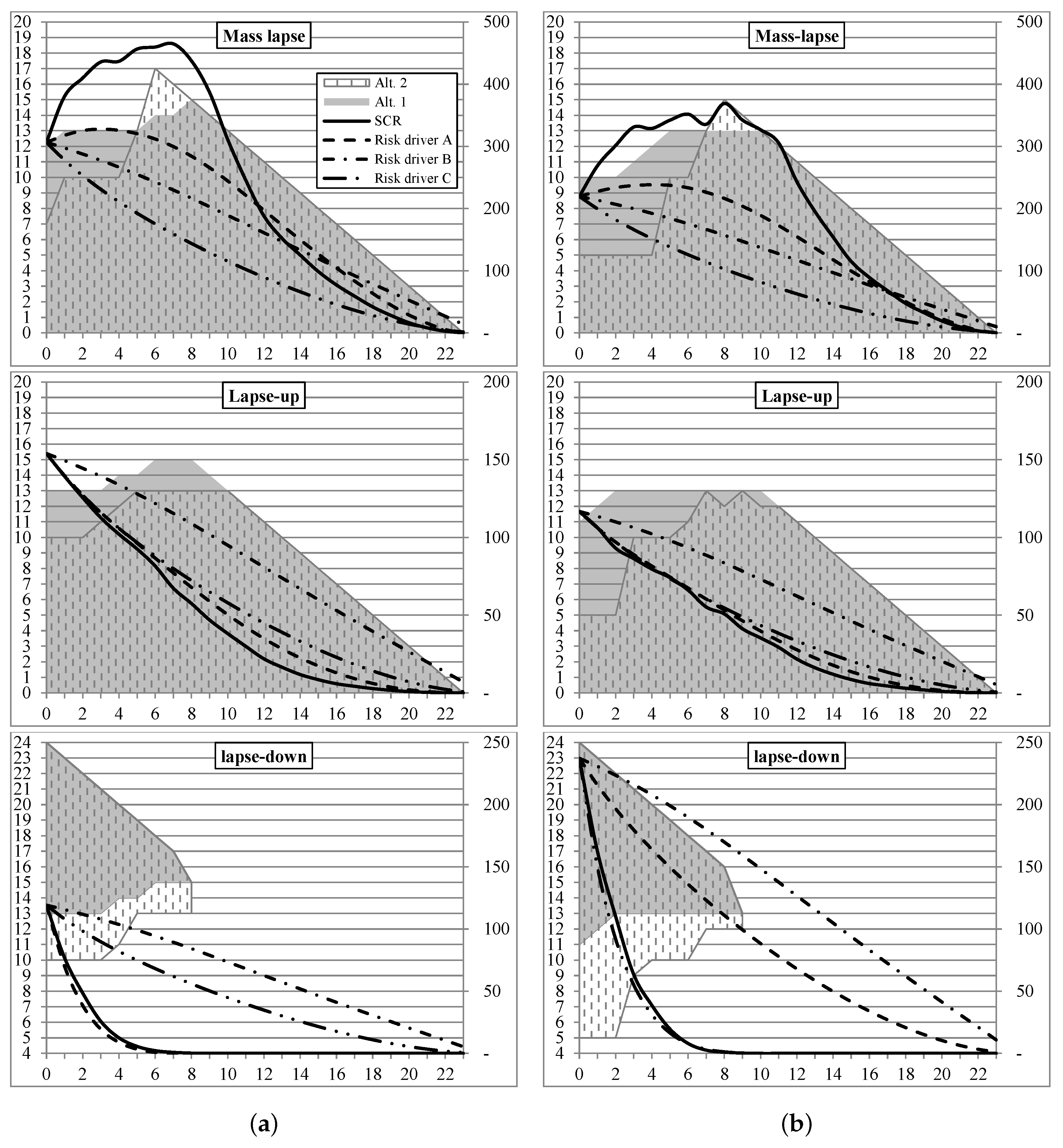
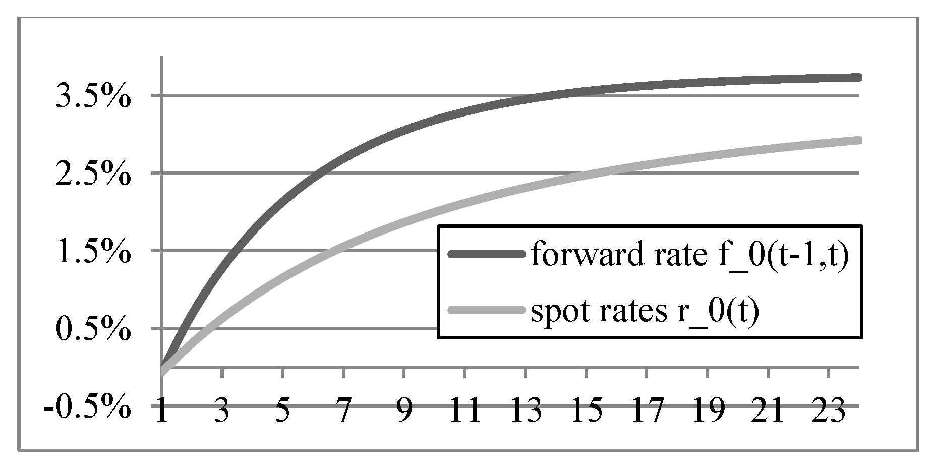
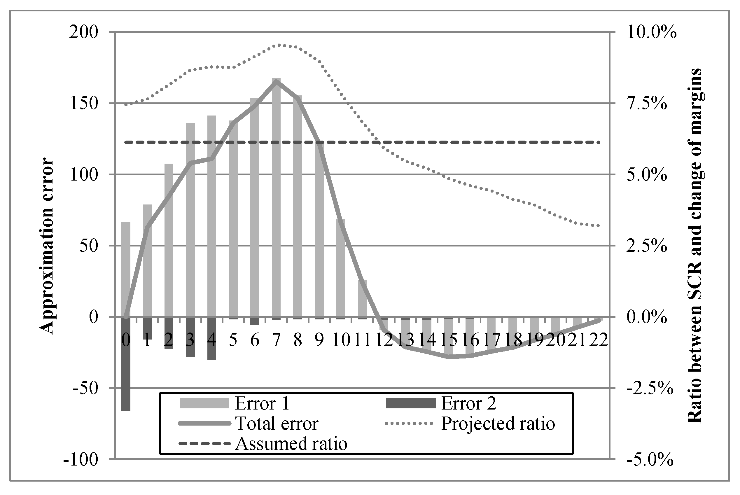
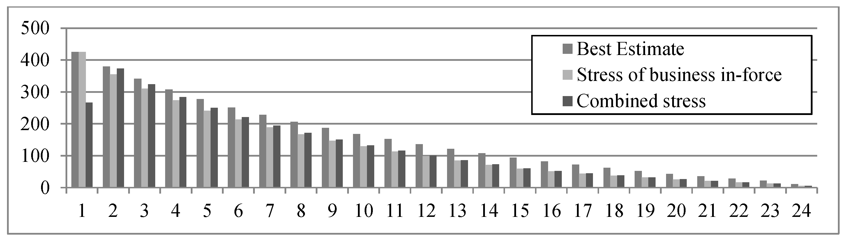
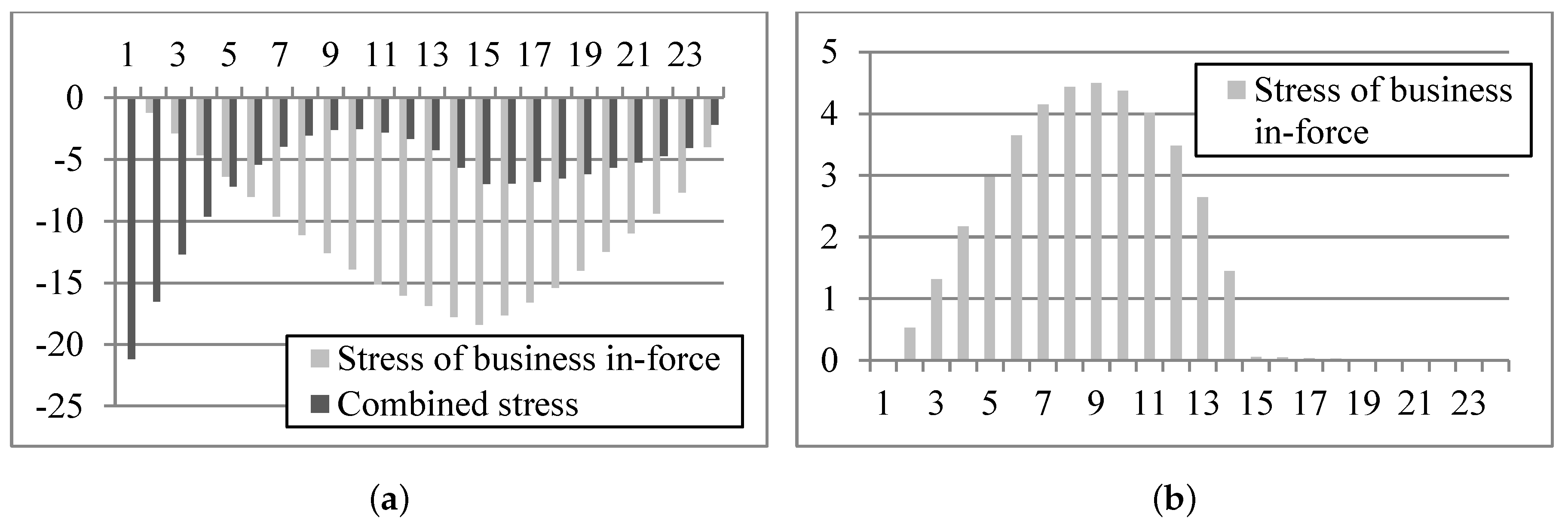
Table A1.
Historic data from the German life insurance market used for deriving the portfolio of insurance contracts.
Table A1.
Historic data from the German life insurance market used for deriving the portfolio of insurance contracts.
| Year | Tariff | Cohort | Net Investment | Administration | Acquisition |
|---|---|---|---|---|---|
| Generation | Return a | Cost Rate a,c | Cost Rate a,d | ||
| 1987 | 0 | - | 7.58 % | 5.80 % | 5.50 % |
| 1988 | 0 | - | 7.32 % | 5.70 % | 5.50 % |
| 1989 | 0 | - | 7.05 % | 5.50 % | 5.50 % |
| 1990 | 0 | - | 6.78 % | 5.40 % | 5.50 % |
| 1991 | 0 | - | 7.44 % | 5.16 % | 5.50 % |
| 1992 | 0 | - | 7.39 % | 4.92 % | 5.50 % |
| 1993 | 0 | 24 | 7.59 % | 4.68 % | 5.50 % |
| 1994 | 0 | 23 | 7.15 % | 4.44 % | 5.50 % |
| 1995 | 1 | 22 | 7.37 % | 4.20 % | 5.50 % |
| 1996 | 1 | 21 | 7.37 % | 4.06 % | 5.52 % |
| 1997 | 1 | 20 | 7.46 % | 3.92 % | 5.54 % |
| 1998 | 1 | 19 | 7.57 % | 3.78 % | 5.56 % |
| 1999 | 1 | 18 | 7.58 % | 3.64 % | 5.58 % |
| 2000 | 1 | 17 | 7.51 % | 3.50 % | 5.60 % |
| 2001 | 2 | 16 | 6.12 % | 3.44 % | 5.60 % |
| 2002 | 2 | 15 | 4.68 % | 3.38 % | 5.60 % |
| 2003 | 2 | 14 | 5.05 % | 3.32 % | 5.60 % |
| 2004 | 3 | 13 | 4.90 % | 3.26 % | 5.60 % |
| 2005 | 3 | 12 | 5.18 % | 3.20 % | 5.60 % |
| 2006 | 3 | 11 | 4.82 % | 3.00 % | 4.90 % |
| 2007 | 4 | 10 | 4.65 % | 2.90 % | 5.20 % |
| 2008 | 4 | 9 | 3.54 % | 2.80 % | 4.90 % |
| 2009 | 4 | 8 | 4.18 % | 2.70 % | 5.20 % |
| 2010 | 4 | 7 | 4.27 % | 2.40 % | 5.10 % |
| 2011 | 4 | 6 | 4.13 % | 2.40 % | 5.00 % |
| 2012 | 5 | 5 | 4.01 % b | 2.40 % | 5.00 % |
| 2013 | 5 | 4 | 4.01 % b | 2.30 % | 5.10 % |
| 2014 | 5 | 3 | 3.91 % b | 2.20 % | 5.00 % |
| 2015 | 6 | 2 | 3.64 % b | 2.30 % | 4.90 % |
| 2016 | 6 | 1 | 3.35 % b | 2.30 % | 4.80 % |
Data is taken from GDV (2017b). Side effects from the increased realization of valuation reserves for the financing of the ZZR have been eliminated. The administration cost rate is given as a percentage of gross written premium income. No data is given for years 1987 to 1994; the missing values are derived by interpolation. The acquisition cost rate is given as a percentage of new business premium sum. No data is given for 1994 and previous years; we use the acquisition cost rate for 1995 also for those years.
References
- Albizzati, Marie-Odile, and Hélyette Geman. 1994. Interest rate risk management and valuation of the surrender option in life insurance policies. Journal of Risk and Insurance 61: 616–37. [Google Scholar] [CrossRef]
- Bacinello, Anna Rita. 2003. Fair valuation of a guaranteed life insurance participating contract embedding a surrender option. Journal of Risk and Insurance 70: 461–87. [Google Scholar] [CrossRef]
- BaFin. 2013. Jahresbericht der bundesanstalt für finanzdienstleistungsaufsicht. Bonn/Frankfurt: BaFin. [Google Scholar]
- BaFin. 2015. Interpretative decisions—Überschussfonds nach Art. 91 der Solvency-II-Richtlinie. Bonn/Frankfurt: BaFin. [Google Scholar]
- Bauer, Daniel, Rüdiger Kiesel, Alexander Kling, and Jochen Ruß. 2006. Risk-neutral valuation of participating life insurance contracts. Insurance: Mathematics and Economics 39: 171–83. [Google Scholar] [CrossRef]
- Berdin, Elia, Helmut Gründl, and Christian Kubitza. 2017. Rising interest rates, lapse risk, and the stability of life insurers. ICIR Working Paper Series. [Google Scholar] [CrossRef]
- Branger, Nicole, and Christian Schlag. 2004. Zinsderivate: Modelle und Bewertung. Berlin: Springer. [Google Scholar]
- Bundesbank. 2017. Zeitreihe BBK01.WZ3089: Aus der Zinsstruktur abgeleitete Renditen für Pfandbriefe mit jährlichen Kuponzahlungen / RLZ 12 Jahr(e)/Monatsendstand. Available online: https://www.bundesbank.de/Navigation/DE/Statistiken/Zeitreihen_Datenbanken/Geld_und_Kapitalmaerkte/geld_und_kapitalmaerkte_details_value_node.html?tsId=BBK01.WZ3089&listId=www_skms_it04b (accessed on 1 December 2017).
- Burkhart, Tobias, Andreas Reuß, and Hans-Joachim Zwiesler. 2015. Participating life insurance contracts under solvency ii: Inheritance effects and allowance for a going concern reserve. European Actuarial Journal 5: 203–44. [Google Scholar] [CrossRef]
- Burkhart, Tobias, Andreas Reuß, and Hans-Joachim Zwiesler. 2017. Allowance for surplus funds under solvency ii: Adequate reflection of risk sharing between policyholders and shareholders in a risk-based solvency framework? European Actuarial Journal 7: 51–88. [Google Scholar] [CrossRef]
- Campbell, Jason, Michael Chan, Kate Li, Louis Lombardi, Lucian Lombardi, Marianne Purushotham, and Anand Rao. 2014. Modeling of Policyholder Behavior for Life Insurance and Annuity products. Schaumburg: Society of Actuaries. [Google Scholar]
- CFO Forum. 2016. Market Consistent Embedded Value Principles. Available online: http://www.cfoforum.nl/downloads/CFO-Forum_MCEV_Principles_and_Guidance_April_2016.pdf (accessed on 1 December 2017).
- Christiansen, Marcus C., and Andreas Niemeyer. 2014. Fundamental definition of the solvency capital requirement in solvency II. Astin Bulletin 44: 501–33. [Google Scholar] [CrossRef]
- Clark, Dominic, Jeremy Kent, and Edward Morgan. 2013. Dynamic Policyholder Behaviour and Management Actions Survey Report. Seattle: Milliman Survey, October 3, 59 p. [Google Scholar]
- EIOPA. 2011. Report on the Fifth Quantitative Impact Study (QIS5) for Solvency II (EIOPA-TFQIS5-11/001). Frankfurt: EIOPA, March 14. [Google Scholar]
- EIOPA. 2015. Guidelines on the Valuation of Technical Provisions (EIOPA-BoS-14/166 EN). Frankfurt: EIOPA, February 2. [Google Scholar]
- Eling, Martin, and Michael Kochanski. 2013. Research on lapse in life insurance: what has been done and what needs to be done? The Journal of Risk Finance 14: 392–413. [Google Scholar] [CrossRef]
- European Commission. 2015. Commission Delegated Regulation (EU) 2015/35. Brussels: European Commission. [Google Scholar]
- European Union. 2009. Directive 2009/138/EC of the European Parliament and of the Council of 25 November 2009 on the Taking-Up and Pursuit of the Business of Insurance and Reinsurance (Solvency II). OJ L 335, 17.12.2009. Brussels: European Union, pp. 1–155. [Google Scholar]
- Feodoria, Mark, and Till Förstemann. 2015. Lethal Lapses: How a Positive Interest Rate Shock Might Stress German Life Insurers. No. 12. Frankfurt: Deutsche Bundesbank. [Google Scholar]
- Führer, Christian, and Arnd Grimmer. 2010. Einführung in die lebensversicherungsmathematik, 2nd ed. Karlsruhe: Verl. Versicherungswirtschaft. [Google Scholar]
- Gatzert, Nadine. 2009. Implicit options in life insurance: An overview. Zeitschrift für Die Gesamte Versicherungswissenschaft 98: 141–64. [Google Scholar] [CrossRef]
- GDV. 2015. Säule I-Anleitung für einzelunternehmen—Eine zusammenfassung der säule I-anforderungen von Solvency II für einzelunternehmen. Berlin: GDV. [Google Scholar]
- GDV. 2017a. Fachkonzept branchensimulationsmodell. Berlin: GDV. [Google Scholar]
- GDV. 2017b. Statistisches Rundschreiben Nr. 0960/2017 (LV): Kennzahlen-mappe 2017—Die deutsche lebensversicherung. Berlin: GDV. [Google Scholar]
- Geneva Association. 2012. Surrenders in the Life Insurance Industry and Their Impact on Liquidity. Geneva: Geneva Association. [Google Scholar]
- Glasserman, Paul. 2010. Monte Carlo Methods in Financial Engineering. New York: Springer. [Google Scholar]
- Grosen, Anders, and Peter Løchte Jørgensen. 2000. Fair valuation of life insurance liabilities: The impact of interest rate guarantees, surrender options, and bonus policies. Insurance: Mathematics and Economics 26: 37–57. [Google Scholar] [CrossRef] [Green Version]
- Kling, Alexander, Frederik Ruez, and Jochen Ruß. 2014. The impact of policyholder behavior on pricing, hedging, and hedge efficiency of withdrawal benefit guarantees in variable annuities. European Actuarial Journal 4: 281–314. [Google Scholar] [CrossRef]
- Kochanski, Michael. 2010. Solvenzkapital für flv unter berücksichtigung von dynamischem storno. Zeitschrift für Die Gesamte Versicherungswissenschaft 99: 689–710. [Google Scholar] [CrossRef]
- Kuo, Weiyu, Chenghsien Tsai, and Wei-Kuang Chen. 2003. An empirical study on the lapse rate: The cointegration approach. Journal of Risk and Insurance 70: 489–508. [Google Scholar] [CrossRef]
- Oechslin, Joachim, Olivier Aubry, Matthias Aellig, Alexander Kappeli, Daniel Bronnimann, Arnaud Tandonnet, and Guillaume Valois. 2007. Replicating embedded options. Life & Pension Risk February 3: 47–52. [Google Scholar]
- Reuß, Andreas, Jochen Ruß, and Jochen Wieland. 2015. Participating life insurance contracts under risk based solvency frameworks: How to increase capital efficiency by product design. In Innovations in Quantitative Risk Management. Springer Proceedings in Mathematics & Statistics. Cham: Springer, vol. 99, pp. 185–208. [Google Scholar]
- Wolfsdorf, Kurt. 1997. Versicherungsmathematik: Teil 1: Personenversicherung. Stuttgart: Vieweg + Teubner Verlag. [Google Scholar]
| 1. | For an overview of the existing literature e.g., see Eling and Kochanski (2013) or Campbell et al. (2014). |
| 2. | For more details concerning the definition of SCR see Christiansen and Niemeyer (2014). |
| 3. | We do not address the allowance of ancillary own funds and eligibility restrictions under the Solvency II framework. Therefore, BOF coincide with Eligible Own Funds. |
| 4. | |
| 5. | See comments given by the German Insurance Association regarding the required segmentation (GDV 2015). |
| 6. | Please note that although this paper concentrates on the option to surrender a contract prior to maturity, those challenges apply to all types of options, e.g., annuitization or premium indexation options. |
| 7. | The actual valuation does not consider new business. However, assumptions regarding expected new business are required to determine the GCR. |
| 8. | For technical reasons, both death and surrender occur at the end of the year. |
| 9. | |
| 10. | The valuation does not include new business and acquisition costs are only relevant for the calculation of the GCR (see Section 3.8.2). |
| 11. | Please note that the part of the commission that has to be repaid in case of surrender is similar but not identical to the Zillmer receivable. |
| 12. | This management rule is in line with common practice but different from Burkhart et al. (2017). |
| 13. | Please note that since the offsetting of different surplus sources is limited to the case of negative investment surplus, it is generally possible to have a positive surplus participation despite a negative raw surplus . |
| 14. | For a more detailed description of the surplus allocation process see Burkhart et al. (2015). |
| 15. | Please note that the Market Consistent Embedded Value framework (CFO Forum 2016) defines the TVFOG from the shareholders’ perspective (based on the PVFP), but in our model framework both approaches result in the same value. |
| 16. | Please note that are not included in the cash flows used to determine BEL (cf. Equation (5)). |
| 17. | SF can easily be combined with the GCR via the ex-post approach. |
| 18. | The rather small value of TVO is in line with current observations from practical applications. |
| 19. | Please note that margins increase from cohorts 16 to 14, 13 to 11, and 10 to 6. |
| 20. | Please note that similar to alt. 1, applying the lapse stresses to the oldest cohort 24 does not change the BEL at all. |
| 21. | |
| 22. | The latter can be traced back to the asymmetry of the profit sharing process in Germany which is reflected in our Monte Carlo valuation framework. Additional surrenders of contracts with fairly high technical interest rates in alt. 1 may reduce losses related to investment returns below the technical interest rate in downside scenarios, but has a smaller impact in upside scenarios. Overall, this has a positive impact on the PVFP that exceeds the loss of future margins. Hence, despite losing additional margins in alt. 1, the insurer is better off due to reduced volume of minimum interest rate guarantees. |
| 23. | For the base case, SCRs and the respective segmentations at time correspond to the results presented in Section 4.2. |
| 24. | For further details regarding the joint impact of increasing interest rates and surrender rates on the insurer’s solvency, see Berdin et al. (2017). |
| 25. | Although the segmentation between alt. 1 and 2 only differs until year 7, error 2 can be observed throughout the projection. This is due to the fact that risk driver A does not allow for dynamic policyholder behavior which slightly affects the change of margin. |
Figure 1.
Development of SCR over time (in € 1000). (a) Base case; (b) Interest rate sensitivity.

Figure 2.
Initial spot rates and forward rates .

Figure 3.
Error due to approximation of using positive change of margins (in € 1000).

Figure 4.
Pre-financing of acquisition costs over time for best estimate and mass lapse stress (in € 1000).
Figure 4.
Pre-financing of acquisition costs over time for best estimate and mass lapse stress (in € 1000).

Figure 5.
Change of pre-financing of uncovered acquisition costs over time for the lapse up and lapse down stress compared to the best estimate (in € 1000). (a) Lapse up stress; (b) Lapse down stress.
Figure 5.
Change of pre-financing of uncovered acquisition costs over time for the lapse up and lapse down stress compared to the best estimate (in € 1000). (a) Lapse up stress; (b) Lapse down stress.

Table 1.
Statutory balance sheet at time .
| Assets | Liabilities |
|---|---|
Table 2.
Insurance contract parameters.
| Tariff | Years of Sale | x | n | G | i | Mortality Table | |||
|---|---|---|---|---|---|---|---|---|---|
| 0 | 1987–1994 | 40 | 25 | € 20,000 | DAV 2008 T a | ||||
| 1 | 1995–2000 | 40 | 25 | € 20,000 | DAV 2008 T | ||||
| 2 | 2001–2003 | 40 | 25 | € 20,000 | DAV 2008 T | ||||
| 3 | 2004–2006 | 40 | 25 | € 20,000 | DAV 2008 T | ||||
| 4 | 2007–2011 | 40 | 25 | € 20,000 | DAV 2008 T | ||||
| 5 | 2012–2014 | 40 | 25 | € 20,000 | DAV 2008 T | ||||
| 6 | 2015–2016 | 40 | 25 | € 20,000 | DAV 2008 T | ||||
| 7 | since 2017 | 40 | 25 | € 20,000 | DAV 2008 T |
This is the German standard mortality table.
Table 3.
Statutory balance sheet at time (in € 1000).
| Assets | Liabilities | ||
|---|---|---|---|
| 1895 | |||
| 988 | |||
| 7067 | |||
| 2546 | |||
Table 4.
Deterministic lapse rates.
| Contract Year m | 1 | 2 | 3 | 4 | 5 | ||
|---|---|---|---|---|---|---|---|
| Deterministic surrender rate |
Table 5.
Parameters for management rules.
| d | |||||||||||
|---|---|---|---|---|---|---|---|---|---|---|---|
| 12 years | 10 years | 5 years |
Table 6.
Financial market parameters.
| Scenario | ||||||
|---|---|---|---|---|---|---|
| Base case | ||||||
| Interest rate sensitivity |
Table 7.
Economic balance sheet at time (in € 1000).
| Base Case | Interest Rate Sensitivity | |||||||
|---|---|---|---|---|---|---|---|---|
| Assets | Liabilities | Assets | Liabilities | |||||
| BOF | 1236 | BOF | 21 | |||||
| BEL | BEL | |||||||
| 2382 | 3259 | |||||||
| 120 | 211 | |||||||
| 2262 | 3048 | |||||||
| () | () | |||||||
Table 8.
Result of segmentation alternatives 1 and 2 (in € 1000).
| k | Alt. 1: | Alt. 2: (Stand-Alone Stress) | |||||||||
|---|---|---|---|---|---|---|---|---|---|---|---|
| Mass Lapse | Lapse Up | Lapse Down | Mass Lapse | Lapse Up | Lapse Down | ||||||
| 24 | −0.79 | - | - | - | −576 | (-) | 42 | (-) | - | (-) | |
| 23 | −1.27 | −0.23 | −0.01 | 0.01 | −576 | (−16.1) | 42 | (−0.5) | 1 | (0.5) | |
| 22 | −1.80 | −0.44 | −0.03 | 0.03 | −580 | (−41.5) | 43 | (−2.0) | 2 | (1.8) | |
| 21 | −2.01 | −0.55 | −0.04 | 0.04 | −560 | (−61.9) | 45 | (−4.0) | 6 | (3.7) | |
| 20 | −2.12 | −0.62 | −0.06 | 0.06 | −522 | (−76.4) | 49 | (−6.1) | 12 | (5.9) | |
| 19 | −2.15 | −0.65 | −0.07 | 0.07 | −463 | (−95.7) | 56 | (−9.0) | 22 | (9.1) | |
| 18 | −2.12 | −0.66 | −0.08 | 0.08 | −382 | (−110.2) | 65 | (−12.1) | 34 | (12.2) | |
| 17 | −2.05 | −0.65 | −0.09 | 0.09 | −280 | (−123.3) | 77 | (−15.2) | 50 | (15.8) | |
| 16 | −1.28 | −0.37 | −0.04 | 0.04 | −158 | (−91.3) | 93 | (−12.7) | 64 | (13.4) | |
| 15 | −1.14 | −0.32 | −0.03 | 0.03 | −72 | (−95.8) | 105 | (−14.5) | 79 | (15.4) | |
| 14 | −1.00 | −0.27 | −0.02 | 0.03 | 23 | (−98.7) | 119 | (−15.6) | 97 | (16.9) | |
| 13 | −0.28 | −0.00 | 0.04 | −0.05 | 124 | (−57.6) | 135 | (−7.9) | 106 | (8.9) | |
| 12 | −0.12 | 0.05 | 0.06 | −0.07 | 185 | (−53.0) | 142 | (−6.7) | 114 | (7.1) | |
| 11 | 0.02 | 0.10 | 0.07 | −0.09 | 243 | (−47.8) | 149 | (−5.2) | 119 | (5.3) | |
| 10 | 0.73 | 0.38 | 0.16 | −0.19 | 297 | (−5.1) | 154 | (5.0) | 113 | (−5.9) | |
| 9 | 0.85 | 0.42 | 0.18 | −0.21 | 304 | (−3.6) | 149 | (5.1) | 106 | (−6.1) | |
| 8 | 0.95 | 0.45 | 0.20 | −0.24 | 305 | (−1.6) | 144 | (5.4) | 100 | (−6.2) | |
| 7 | 1.05 | 0.48 | 0.22 | −0.26 | 306 | (−0.5) | 138 | (5.2) | 94 | (−5.4) | |
| 6 | 1.13 | 0.51 | 0.23 | −0.29 | 305 | (2.4) | 134 | (5.8) | 88 | (−5.8) | |
| 5 | 1.74 | 0.75 | 0.33 | −0.41 | 300 | (37.9) | 129 | (15.7) | 71 | (−16.8) | |
| 4 | 1.75 | 0.76 | 0.35 | −0.45 | 257 | (37.7) | 114 | (15.8) | 55 | (−17.2) | |
| 3 | 1.74 | 0.76 | 0.38 | −0.48 | 219 | (39.9) | 98 | (17.4) | 35 | (−19.2) | |
| 2 | 2.49 | 1.02 | 0.54 | −0.71 | 178 | (87.5) | 81 | (38.0) | −8 | (−43.9) | |
| 1 | 2.39 | 0.96 | 0.56 | -0.76 | 85 | (84.6) | 42 | (42.0) | −57 | (−49.3) | |
Table 9.
Change of BEL () and its components (in € 1000).
| Change of | Mass Lapse | Lapse Up | Lapse Down | ||||||||
|---|---|---|---|---|---|---|---|---|---|---|---|
| All | Alt. 1 | Alt. 2 | All | Alt. 1 | Alt. 2 | All | Alt. 1 | Alt. 2 | |||
| BEL | −576 | 185 | 306 | 42 | 135 | 154 | −57 | 97 | 119 | ||
| 3842 | 5303 | 4207 | 2366 | 2542 | 2440 | −3057 | 183 | 64 | |||
| −3232 | −4645 | −3755 | −2115 | −2285 | −2210 | 2763 | −169 | −80 | |||
| −1186 | −473 | −146 | −209 | −122 | −76 | 237 | 83 | 135 | |||
| (3.5%) | (4.9%) | (2.3%) | (2.6%) | (0.8%) | (1.1%) | ||||||
Table 10.
Cost-of-capital resulting from projected and approximated SCRs (in € 1000).
| SCR Projection | SCR Approximation (In % of Explicit SCR Projection) | ||||||
|---|---|---|---|---|---|---|---|
| Risk Driver A | Risk Driver B | Risk Driver C | |||||
| (Base case) | |||||||
| Mass lapse | 324 | 266 | () | 233 | () | 161 | () |
| Lapse up | 66 | 74 | () | 117 | () | 81 | () |
| Lapse down | 17 | 16 | () | 91 | () | 63 | () |
| Lapse | 324 | 266 | () | 233 | () | 161 | () |
| (Interest rate sensitivity) | |||||||
| Mass lapse | 281 | 201 | () | 169 | () | 115 | () |
| Lapse up | 54 | 57 | () | 90 | () | 61 | () |
| Lapse down | 38 | 35 | () | 183 | () | 124 | () |
| Lapse | 283 | 202 | () | 183 | () | 124 | () |
Table 11.
Cost-of-capital (in % of SCR projection) resulting from interpolation of SCRs (in € 1000).
Table 11.
Cost-of-capital (in % of SCR projection) resulting from interpolation of SCRs (in € 1000).
| Scenario | Mass Lapse | Lapse Up | Lapse Down | Lapse | ||||
|---|---|---|---|---|---|---|---|---|
| Base case | 303 | () | 71 | () | 22 | () | 303 | () |
| Interest rate sensitivity | 283 | () | 57 | () | 49 | () | 284 | () |
Table 12.
BOF and SCR under different stress assumptions regarding the GCR (in € 1000).
| Assumptions Regarding GCR | BOF | Change of BOF in Case of | |||||||||
|---|---|---|---|---|---|---|---|---|---|---|---|
| Best Estimate | Mass Lapse | Lapse Up | Lapse Down | ||||||||
| GCR | Total | GCR | Total | GCR | Total | GCR | Total | ||||
| Best estimate | 3445 | 3520 | 0 | −493 | 0 | −208 | 0 | −132 | |||
| Stress of business in-force | 3445 | 3520 | −556 | −825 | −184 | −342 | 32 | −115 | |||
| Combined stress | 3445 | 3520 | −632 | −878 | −118 | −284 | n/a | n/a | |||
Table 13.
Change of relevant BOF components in the mass lapse scenario (in € 1000).
| Calculation of Surplus Funds | BOF | Change of BOF | |||||||
|---|---|---|---|---|---|---|---|---|---|
| Best Estimate | Mass Lapse | ||||||||
| SF | Total | SF | Total | SF | Total | ||||
| based on best estimate valuation | 3513 | 4749 | 3513 | 4452 | 0 | ||||
| without change of due to stress | 3513 | 4749 | 3543 | 4482 | |||||
| with change of due to stress | 3513 | 4749 | 3321 | 4260 | |||||
| (Terminal bonuses in year 1) | (411) | (633) | () | ||||||
© 2018 by the author. Licensee MDPI, Basel, Switzerland. This article is an open access article distributed under the terms and conditions of the Creative Commons Attribution (CC BY) license (http://creativecommons.org/licenses/by/4.0/).
Share and Cite
MDPI and ACS Style
Burkhart, T. Surrender Risk in the Context of the Quantitative Assessment of Participating Life Insurance Contracts under Solvency II. Risks 2018, 6, 66. https://doi.org/10.3390/risks6030066
AMA Style
Burkhart T. Surrender Risk in the Context of the Quantitative Assessment of Participating Life Insurance Contracts under Solvency II. Risks. 2018; 6(3):66. https://doi.org/10.3390/risks6030066
Chicago/Turabian StyleBurkhart, Tobias. 2018. "Surrender Risk in the Context of the Quantitative Assessment of Participating Life Insurance Contracts under Solvency II" Risks 6, no. 3: 66. https://doi.org/10.3390/risks6030066
Note that from the first issue of 2016, this journal uses article numbers instead of page numbers. See further details here.