Masked Instability: Within-Sector Financial Risk in the Presence of Wealth Inequality

Abstract

We investigate masked financial instability caused by wealth inequality. When an economic sector is decomposed into two subsectors that possess a severe wealth inequality, the sector in entirety can look financially stable while the two subsectors possess extreme financially instabilities of opposite nature, one from excessive equity, the other from lack thereof. The unstable subsector can result in further financial distress and even trigger a financial crisis. The market instability indicator, an early warning system derived from dynamical systems applied to agent-based models, is used to analyze the subsectoral financial instabilities. Detailed mathematical analysis is provided to explain what financial instabilities can arise amid seemingly stable economy and positive market data. The theoretical conjecture is verified by historical macroeconomic time series of the United States households among whom a substantial wealth inequality has been officially confirmed.

1. Introduction

It has been a decade since the outbreak of the 2007–2010 United States Subprime Mortgage Crisis that was followed by the 2009–2014 European Sovereign Debt Crisis. The two financial crises resulted in the Great Recession that suppressed the global economy for several years. The U.S. economy seems to have fully recovered in terms of economic and financial indicators. For example, the labor market is near full employment with the unemployment rate at 3.8% as of June 2018 according to Bureau of Labor Statistics (2018), and stock indices hit historical highs in the first quarter of the same year (e.g., Bloomberg 2018).

However, reports have been made that the Great Recession exacerbated the uneven wealth distribution in the United States (e.g., Kochhar and Cilluffo 2017; Wolff 2014), and, at the same time, wealth inequality has been addressed as an increasing social problem by both organizations and scholars (e.g., Congressional Budget Office 2016; Organization for Economic Cooperation and Development 2016; Saez and Zucman 2016). Concerns about wealth inequality is not a phenomenon restricted to the United States as can be seen from the frenzied worldwide reaction to the publication of Capital in the Twenty-First Century by Piketty (2014).

We investigate how wealth inequality can affect correct assessment of financial stability of an economic sector by showing that, when an economic sector is divided into two subsectors by extreme concentration of wealth and lack thereof, it may mask risk exposures within subsectors that are not readily observable from the aggregate. This article is the latest installment of our ongoing research about the role of borrowing capacity in determining the financial instability, and, as such, we are interested in whether the aggregate borrowing capacity could misrepresent the reality in the presence of extreme wealth inequality. There are many factors that determine the borrowing capacity of an economic agent, but, for households, it is the current level of wealth, income, and debt that are the most important and easily quantifiable ones. According to the Survey of Consumer Finances (2017) (SCF), the top 10% of the United States households possess more than 75% of the total wealth and about half of the total income while the consumer debt, including a dangerously high level of student loans as pointed by many (e.g., Foroohar 2017), reached a new peak in 2017 Q4 (Federal Reserve Bank of New York 2018). This could create an uneven distribution of borrowing capacity within the households, hence different levels of financial instability as well.

There are many definitions of financial stability and financial instability (e.g., Alawode and Al Sadek 2008), yet they all have a common theme: financial stability entails resilience and shock-absorbing capacity while financial instability involves impairment of the financial system and its adverse effect on economic activity. The last condition often leads to the definition of systemic risk, which is summarized by Freixas et al. (2015) as an unusual financial shock that causes strong negative shocks to the real economy. We are interested in the financial (in)stability of a single economic agent rather than the system itself, hence we give our own definition: the financial stability of an agent is a state in which the agent absorbs a shock, not necessarily negative, on its wealth to keep steady its outgoing cash flows. Therefore, when an agent goes through financial instability or is financially unstable, a shock on its wealth is transmitted to another agent or even propagates throughout the system. Examples of such shock transmissions are default on a loan payment for a negative shock and over-investment for a positive shock. It should be noted that unlike the post-subprime crisis works by Rajan (2010) and Kumhof and Rancière (2010) that study the link between wealth inequality and financial crisis or those of Atkinson and Morelli (2011) and Bordo and Meissner (2012) that find no evidence of such a linkage, our goal is not to prove or disprove the existence of any nexus between wealth inequality and financial instability leading to a crisis but to show that wealth inequality can mask financial inequalities within an economic sector that appears financially stable.

We use the market instability indicator, an early warning system proposed by Choi and Douady (2012), to quantify the level of financial instability of the United States households and nonprofit institutions serving households (HNISH) and its subsectors. HNISH is chosen because its macroeconomic time series are available on Integrated Macroeconomic Accounts for the United States (2018) and the Survey of Consumer Finances (2017) confirms an extreme wealth inequality within the sector, and hence serves our purpose well.

The rest of the paper is organized as follows. Section 2 explains the background and setup of the work, and Section 3 presents the mathematical details of the impact of wealth inequality on financial stability. Section 4 is devoted to a case study of the United States HNISH, and Section 5 provides the conclusions.

2. Basic Setup

Given an economy, consider its domestic part and divide it into four aggregates called agents, households (H), companies (C), financial institutions not restricted to banks (F), and government (G), indexed from 1 to 4 in that order. For each agent i, define its wealth (commonly known as asset) $w_i$ as the sum of its equity and debt, and the total wealth of the economy at time t as the vector $w\left(t\right)=(w_1\left(t\right),\cdots ,w_4\left(t\right))$, all in chained currency. The market instability indicator of the system is defined to be the spectral radius of the Jacobian matrix $B\left(t\right)={\left(b_{ij}\left(t\right)\right)}_{1\le i,j\le 4}$ of a differentiable function $f:{\mathbb{R}}^4⟶{\mathbb{R}}^4$ such that $f\left(w\right(t\left)\right)=w(t+1)$. Higher market instability indicator implies more financial instability of the system. Let $F_{ij}\left(t\right)>0$ be the fund transferred from agent j to i1 and $F_{ii}\left(t\right)$ the internal return on the invested asset portion of $w_i\left(t\right)$, also in chained currency. With these notations,

$$w_i(t+1)=w_i\left(t\right)+\sum _{j=1}^4{F}_{ij}\left(t\right)-\sum _{k\ne i}^4{F}_{ki}\left(t\right).$$

(1)

The elasticity coefficient $a_{ij}$, defined as

$$a_{ij}={\displaystyle \frac{\partial F_{ij}}{\partial w_j}}\mathrm{for}i\ne j,$$

(2)

measures how susceptible the outgoing cash flow $F_{ij}$ is to a change in $w_j$. Similarly, we define $a_{ii}$ as the change rate of internal return on invested asset $F_{ii}\left(t\right)$ with respect to $w_i\left(t\right)$, so for all i and j

$$a_{ij}\left(t\right)={\displaystyle \frac{\partial F_{ij}\left(t\right)}{\partial w_j\left(t\right)}}.$$

(3)

We further assume that changes in one agent’s wealth do not affect the outgoing cash flows of others, hence

$${\displaystyle \frac{\partial F_{ij}}{\partial w_k}}=0\mathrm{if}j\ne k.$$

(4)

It can be proved that $a_{ij}$ differs from the Jacobian component $b_{ij}$ only on the diagonal,

$$\begin{array}{c}{b}_{ii}=1+a_{ii}-\sum _{k\ne i}^4{a}_{ki},\mathrm{and}\hfill \end{array}$$

(5)

$$\begin{array}{c}{b}_{ij}=a_{ij}\mathrm{for}i\ne j.\hfill \end{array}$$

(6)

By definition

$$b_{ii}\left(t\right)=\frac{\partial w_i(t+1)}{\partial w_i\left(t\right)}$$

(7)

and the market instability indicator of agent i (as opposed to the system) is $|b_{ii}|$. In dynamical systems, the threshold that determines the stability type of an equilibrium is 1. More precisely, if x is a fixed point of a dynamical system $g:{\mathbb{R}}^n⟶{\mathbb{R}}^n$, then x is a stable fixed point if $\rho \left(x\right)<1$ and unstable fixed point if $\rho \left(x\right)>1$ where $\rho \left(x\right)$ is the spectral radius of the Jacobian matrix $Dg\left(x\right)$. Therefore, agent i is financially stable if $|b_{ii}\left(t\right)|<1$ and financially unstable if $|b_{ii}\left(t\right)|>1$.

However, it is not convenient to use this version of sectoral market instability indicator with real data because $w_i(t+1)$ is a function of $w_i\left(t\right)$ and other cash flows, so it is not possible to directly calculate the partial derivative of $w_i(t+1)$ with respect to $w_i\left(t\right)$. We derive an alternative version of $b_{ii}\left(t\right)$ using time derivatives of wealth and cash flows. Assume that F (agent 3) is the sole creditor to all other agents and denote by $F_{3i}$2 the debt payment by agent i to F. For all agents other than F (i.e., $i\ne 3$), the cash flow $F_{3i}\left(t\right)$ consists of two components, what it actually pays and what it fails to pay. We call the former ${\alpha }_i$ and latter ${\delta }_i$, hence

$$F_{3i}\left(t\right)={\alpha }_i\left(t\right)+{\delta }_i\left(t\right).$$

(8)

The new loan $F_{i3}\left(t\right)$ and net new loan ${\nu }_i\left(t\right)$ taken during $[t,t+1]$ are, respectively,

$$F_{i3}\left(t\right)={\nu }_i\left(t\right)+{\delta }_i\left(t\right)$$

(9)

and

$${\nu }_i\left(t\right)=D_i(t+1)-D_i\left(t\right)+{\alpha }_i\left(t\right).$$

(10)

Now, we express the elasticity coefficient $a_{ij}\left(t\right)$ in terms of time derivatives,

$$a_{ij}\left(t\right)={\displaystyle \frac{{F_{ij}}^{\prime }\left(t\right)}{{w_j}^{\prime }\left(t\right)}},$$

(11)

where “ ′ ” denotes the time derivative. This is derived by applying chain rule and Equation (4) to ${F_{ij}}^{\prime }\left(t\right)$,

$${\displaystyle \frac{d{F}_{ij}}{dt}}=\sum _k{\displaystyle \frac{\partial F_{ij}}{\partial w_k}}·{\displaystyle \frac{d{w}_k}{dt}}={\displaystyle \frac{\partial F_{ij}}{\partial w_j}}·{\displaystyle \frac{d{w}_j}{dt}}.$$

(12)

With these notations, differentiate $w(t+1)$ with respect to time. By Equations (6), (4), and (11), we get

$$\begin{array}{cc}\hfill {w_i}^{\prime }(t+1)& =\sum _j{\displaystyle \frac{\partial w_i(t+1)}{\partial w_j\left(t\right)}}\dot{}{\displaystyle \frac{d{w}_j\left(t\right)}{dt}}\hfill \\ & =b_{ii}\left(t\right){w_i}^{\prime }\left(t\right)+\sum _{j\ne i}{b}_{ij}\left(t\right){w_j}^{\prime }\left(t\right)\hfill \\ & =b_{ii}\left(t\right){w_i}^{\prime }\left(t\right)+\sum _{j\ne i}{a}_{ij}\left(t\right){w_j}^{\prime }\left(t\right)\hfill \\ & =b_{ii}\left(t\right){w_i}^{\prime }\left(t\right)+\sum _{j\ne i}{F_{ij}}^{\prime }\left(t\right).\hfill \end{array}$$

(13)

Hence,

$$\begin{array}{cc}\hfill {\displaystyle \frac{{w_i}^{\prime }(t+1)}{{w_i}^{\prime }\left(t\right)}}& =b_{ii}\left(t\right)+\sum _{j\ne i}{\displaystyle \frac{{F_{ij}}^{\prime }\left(t\right)}{{w_i}^{\prime }\left(t\right)}}\hfill \\ & =b_{ii}\left(t\right)+\sum _{j\ne i,3}{\displaystyle \frac{{F_{ij}}^{\prime }\left(t\right)}{{w_i}^{\prime }\left(t\right)}}+{\displaystyle \frac{{F_{i3}}^{\prime }\left(t\right)}{{w_i}^{\prime }\left(t\right)}}\hfill \\ & =b_{ii}\left(t\right)+\sum _{j\ne i,3}{\displaystyle \frac{{F_{ij}}^{\prime }\left(t\right)}{{w_i}^{\prime }\left(t\right)}}+{\displaystyle \frac{{{\nu }_i}^{\prime }\left(t\right)}{{w_i}^{\prime }\left(t\right)}}+{\displaystyle \frac{{{\delta }_i}^{\prime }\left(t\right)}{{w_i}^{\prime }\left(t\right)}},\hfill \end{array}$$

which subsequently yields

$$b_{ii}\left(t\right)={\displaystyle \frac{{w_i}^{\prime }(t+1)}{{w_i}^{\prime }\left(t\right)}}-\sum _{j\ne i,3}{\displaystyle \frac{{F_{ij}}^{\prime }\left(t\right)}{{w_i}^{\prime }\left(t\right)}}-{\displaystyle \frac{{{\nu }_i}^{\prime }\left(t\right)}{{w_i}^{\prime }\left(t\right)}}-{\displaystyle \frac{{{\delta }_i}^{\prime }\left(t\right)}{{w_i}^{\prime }\left(t\right)}}.$$

(14)

Each of the negative terms in Equation (14) represents the ratio of velocities—the velocity of a cash inflow and that of the wealth—which compares the movement of cash inflow and wealth, and subtracting them in aggregate is to get rid ${w_i}^{\prime }(t+1)$ of the contribution that are not from $w_i\left(t\right)$ to get Equation (7).

The last term in Equation (14) plays an important role in determining the financial instability level and defined to be the default elasticity of agent i at time t,

$${\Delta }_i\left(t\right)={\displaystyle \frac{{{\delta }_i}^{\prime }\left(t\right)}{{w_i}^{\prime }\left(t\right)}}.$$

(15)

When dealing with discrete time series such as quarterly macroeconomic data, the time derivatives are to be substituted by difference quotient,

$$\begin{array}{cc}\hfill {w_i}^{\prime }\left(t\right)& ={\displaystyle \frac{w_i\left(t\right)-w_i(t-1)}{t-(t-1)}}=w_i\left(t\right)-w_i(t-1)\mathrm{and}\hfill \end{array}$$

(16)

$$\begin{array}{cc}\hfill {F_{ij}}^{\prime }\left(t\right)& ={\displaystyle \frac{F_{ij}\left(t\right)-F_{ij}(t-1)}{t-(t-1)}}=F_{ij}\left(t\right)-F_{ij}(t-1).\hfill \end{array}$$

(17)

This modification will be used with real data in Section 4.

3. Wealth Inequality and Financial Stability

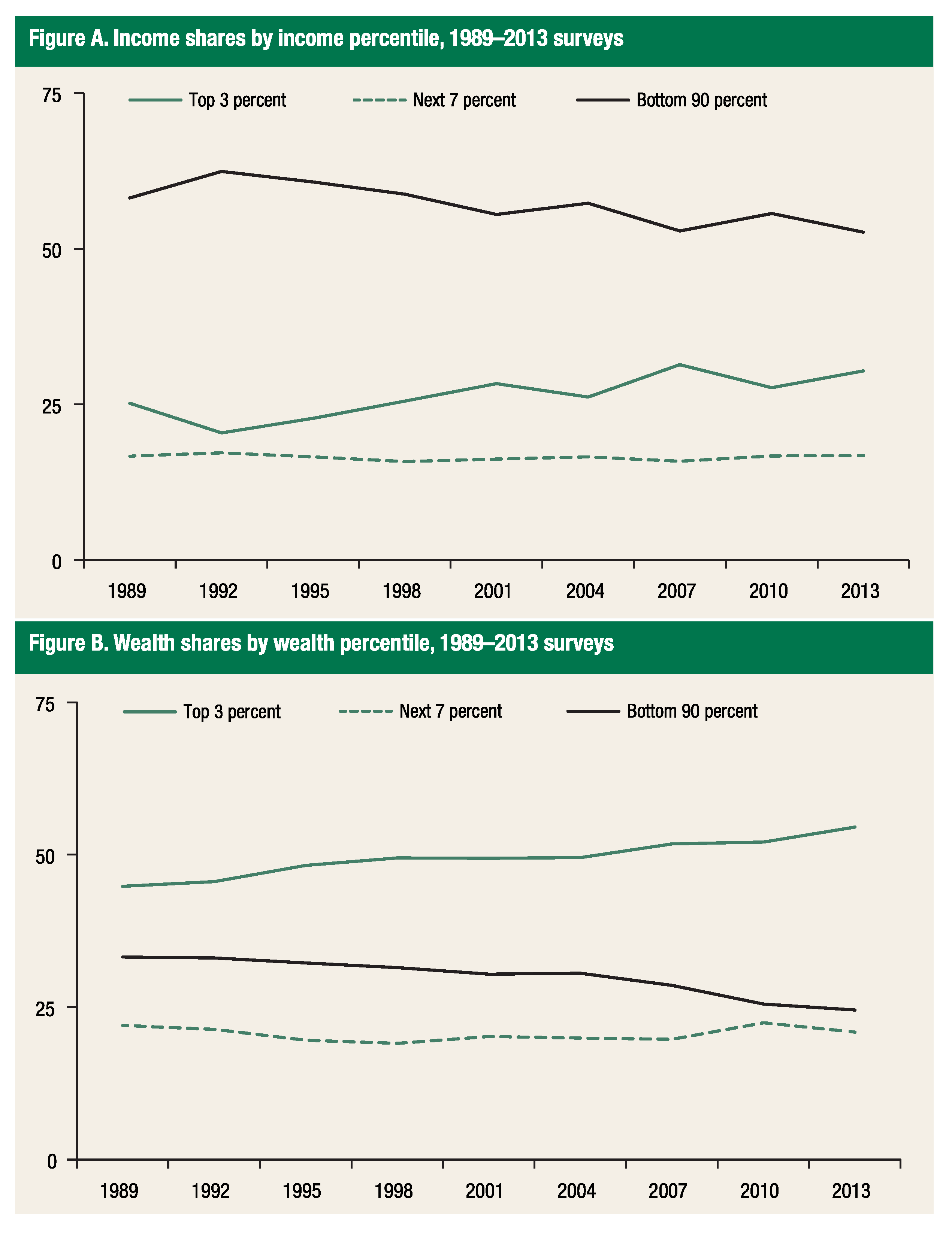
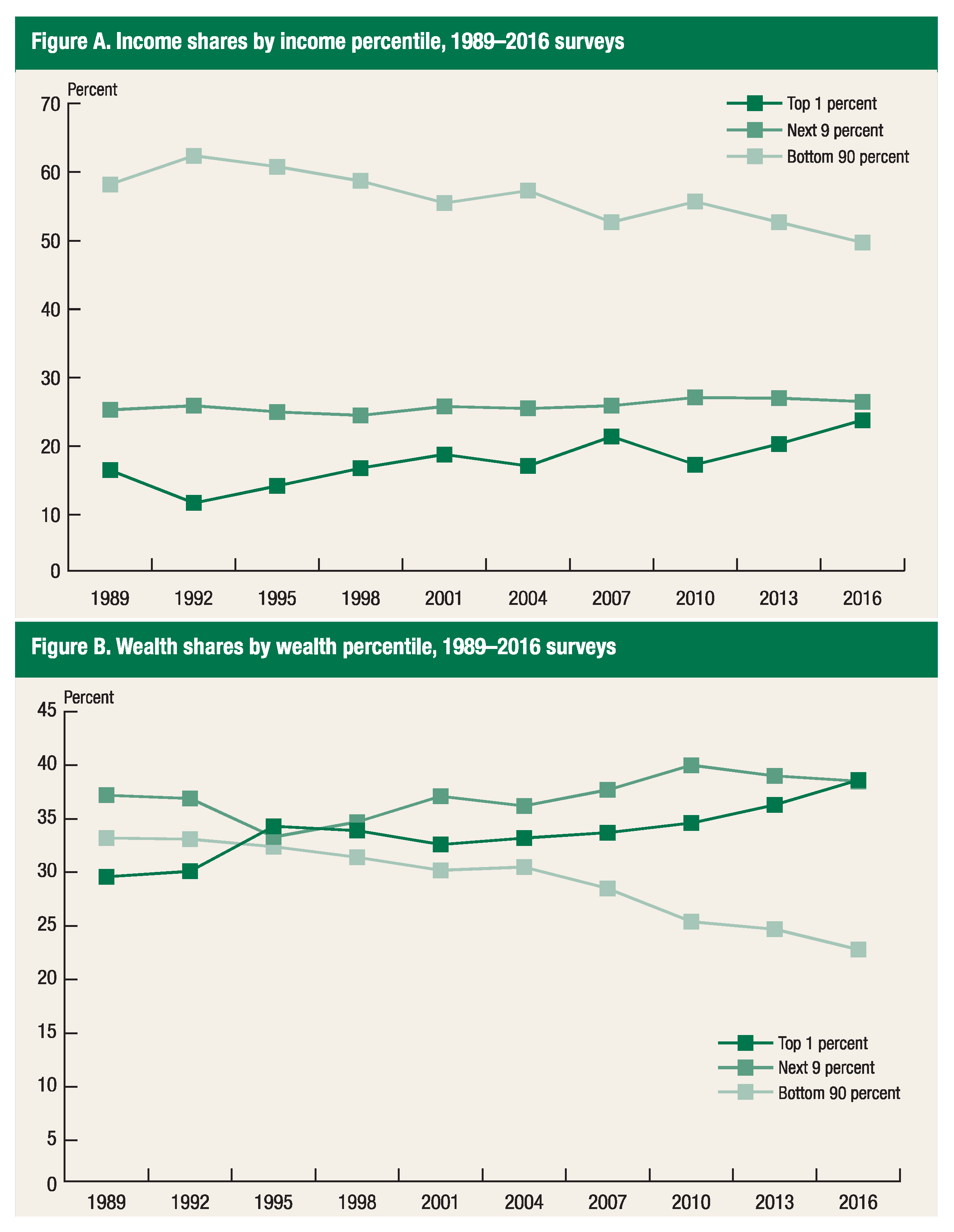
Ten years after the demise of Lehman Brothers that epitomizes the 2007–2010 U.S. subprime mortgage crisis, the United States economy seems to have fully recovered. The employment is nearly full and the current economic expansion, at eight years and ten months as of 1 May 2018, just broke the record to become the second longest in history (Chandra and Golle 2018). Despite this optimistic news, recent Survey of Consumer Finances (2017) shows that the wealth inequality in the U.S. household sector has grown wider since the time of the previous survey, and now the top 10% own more than 75% of the total wealth (Figure 1 and Figure 2).

To model and investigate the impact of this wealth inequality on the financial stability of the households sector H, we divide it into two subsectors, the rich (agent r) and the poor (agent p). We further assume that the rich get richer and the poor get poorer, both with acceleration, which mathematically is expressed as ${w_r}^{\prime }\left(t\right)>0,{w_r}^{″}\left(t\right)>0$ and ${w_p}^{\prime }\left(t\right)<0,{w_p}^{″}\left(t\right)<0$. This assumption is justified by the wealth share changes in the survey. We also assume that the consumption $F_{2r}$ and $F_{2p}$ have reached a full capacity in the sense that the rich do not want to spend more than they do now, and the poor cannot reduce any more the basic cost of living. The assumption on the rich group intuitively makes sense from decreasing marginal propensity to consume (MPC), and is justified by the recent result of Carroll et al. (2017) that the aggregate MPC can differ greatly across wealth and income distribution and wealthy households with high income have low MPCs.

By Equation (5),

$$\begin{array}{c}{b}_{rr}=1+a_{rr}-a_{2r}-a_{3r}-a_{4r},\mathrm{and}\hfill \end{array}$$

(18)

$$\begin{array}{c}{b}_{pp}=1+a_{pp}-a_{2p}-a_{3p}-a_{4p}\hfill \end{array}$$

(19)

The biggest portion of income for the rich tends to be the return on investment, therefore $a_{rr}$ is relatively big and positive. The biggest portion of income for the poor is wages and the return on invested asset is a very small part of $w_p$, which implies $a_{pp}\approx 0$. By our assumption, the consumption for both groups are near a limit with little change, hence both $a_{2r}$ and $a_{2p}$ are negligible. When a borrower’s wealth increases, the lenders often offer more favorable perquisites such as lower interest rates and reduced fees, while decreased wealth results in harsher borrowing conditions such as higher interest rates and minimum balance. This argument on the vicious cycle for the poor and virtuous counterpart for the rich is in line with well-established theories on debt dynamics (e.g., Hart and Moore 1998), asymmetric information (e.g., Akerlof 1970), and financial accelerator (e.g., Bernanke et al. 1999). Therefore, we can assert that

$$a_{3i}={\displaystyle \frac{\partial F_{3i}}{\partial w_i}}<0,i=r,p.$$

(20)

Our assumption on decreasing concave wealth function $w_p\left(t\right)$ can be, without loss of generality, extended such that the poor are highly leveraged with little equity and a small decrease in their wealth can result in a precipitous increase in loan payment obligation and even failure to pay.3 This implies $a_{3p}\ll -1$. As for tax, the rich get various forms of deduction and the poor do not pay much to begin with, so the change in tax with respect to income change would not be significant for either group.4 Therefore,

$$b_{rr}\approx 1+a_{rr}-a_{3r}\gg 1\mathrm{and}{b}_{pp}\approx 1-a_{3p}\gg 1.$$

(21)

The size of the market instability indicator implies that both subsectors of households are financially unstable,5 the rich from excess wealth and the poor lack thereof. Highly indebted households are vulnerable to shocks on their wealth, e.g., drop in housing value, the rise of interest rate on loans, and reduced income from layoffs, to name a few. Such events can cause a financial instability contagion along the feedback loop formed by inter-agent cash flows as explained in Castellacci and Choi (2014), and even trigger a financial crisis similar to the 2007–2010 U.S. subprime mortgage crisis. The rich with excessive capital would look for investment opportunities and this can create bubbles outside their economy just like in the emerging market after the 2008 global financial crisis. However, the households as a single sector can appear financially stable despite these dormant seeds of further turmoil because the subsectoral instabilities of opposite causes can ‘offset’ each other.

We use Equation (14) to explain this mathematically. With subsectors r and p, Equation (14) can be written as follows:

$$\begin{array}{cc}\hfill b_{11}\left(t\right)& ={\displaystyle \frac{{w_1}^{\prime }(t+1)}{{w_1}^{\prime }\left(t\right)}}-{\displaystyle \frac{{F_{12}}^{\prime }\left(t\right)}{{w_1}^{\prime }\left(t\right)}}-{\displaystyle \frac{{F_{14}}^{\prime }\left(t\right)}{{w_1}^{\prime }\left(t\right)}}-{\displaystyle \frac{{{\nu }_1}^{\prime }\left(t\right)}{{w_1}^{\prime }\left(t\right)}}-{\displaystyle \frac{{{\delta }_i}^{\prime }\left(t\right)}{{w_i}^{\prime }\left(t\right)}}\hfill \\ & ={\displaystyle \frac{{w_r}^{\prime }(t+1)+{w_p}^{\prime }(t+1)}{{w_r}^{\prime }\left(t\right)+{w_p}^{\prime }\left(t\right)}}-{\displaystyle \frac{{F_{r2}}^{\prime }\left(t\right)+{F_{p2}}^{\prime }\left(t\right)}{{w_r}^{\prime }\left(t\right)+{w_p}^{\prime }\left(t\right)}}-{\displaystyle \frac{{F_{r4}}^{\prime }\left(t\right)+{F_{p4}}^{\prime }\left(t\right)}{{w_r}^{\prime }\left(t\right)+{w_p}^{\prime }\left(t\right)}}\hfill \\ & -{\displaystyle \frac{{{\nu }_r}^{\prime }\left(t\right)+{{\nu }_p}^{\prime }\left(t\right)}{{w_r}^{\prime }\left(t\right)+{w_p}^{\prime }\left(t\right)}}-{\displaystyle \frac{{{\delta }_r}^{\prime }\left(t\right)+{{\delta }_p}^{\prime }\left(t\right)}{{w_r}^{\prime }\left(t\right)+{w_p}^{\prime }\left(t\right)}}.\hfill \end{array}$$

(22)

We complement the previous assumptions with the following. First, the rich accumulate wealth much faster than the poor such that it mathematically means ${w_1}^{\prime }\left(t\right)>0$ and ${w_1}^{\prime }(t+1)/{w_1}^{\prime }\left(t\right)>1$. Second, the total income including wages and government benefit remain flat. In the Survey of Consumer Finances (2017), the income shares of the top 1% and bottom 90% are almost mirror images of each other, while that of the remaining 9% remains nearly constant, therefore this assumption is reasonable. This means that most of the wealth increase is due to return on investment $F_{11}$. The second assumption on income mathematically means ${F_{12}}^{\prime }\left(t\right)\approx 0,{F_{14}}^{\prime }\left(t\right)\approx 0$. Finally, no more net new loans are taken because the rich do not need it, and the poor cannot afford it. Then,

$$\begin{array}{cc}\hfill b_{11}\left(t\right)& \approx {\displaystyle \frac{{w_1}^{\prime }(t+1)}{{w_1}^{\prime }\left(t\right)}}-{\displaystyle \frac{0}{{w_1}^{\prime }\left(t\right)}}-{\displaystyle \frac{0}{{w_1}^{\prime }\left(t\right)}}-{\displaystyle \frac{0}{{w_1}^{\prime }\left(t\right)}}-{\displaystyle \frac{{{\delta }_i}^{\prime }\left(t\right)}{{w_i}^{\prime }\left(t\right)}}\hfill \end{array}$$

(23)

$$\begin{array}{c}={\displaystyle \frac{{w_1}^{\prime }(t+1)}{{w_1}^{\prime }\left(t\right)}}-{\displaystyle \frac{{{\delta }_r}^{\prime }\left(t\right)+{{\delta }_p}^{\prime }\left(t\right)}{{w_1}^{\prime }\left(t\right)}}\hfill \end{array}$$

(24)

The rich are solvent and liquid enough to rarely default on debt payments while the poor are highly leveraged and susceptible to negative shock on wealth, which implies ${{\delta }_r}^{\prime }=0$ and ${{\delta }_p}^{\prime }>0$. Therefore, $b_{11}\left(t\right)$ is by Equation (27) the difference of two positive numbers, and, as a result, $|b_{11}|$ can become far smaller than $|b_{rr}|$ and $|b_{pp}|$ measured separately, making the households appear financially stable while its two subsectors are not.

This is an extreme case analysis with assumption on constant consumption and tax payment (which are consequences of flat income and benefit assumption used for Equation (23)), but even in real life the two cash flows could stay relatively steady compared with other ones. Therefore, when other assumptions on wealth and debt are satisfied, it is possible for the households of an economy to appear financially stable and safe from economic distress while it has an unstable subsector that can create asset bubbles (and a crisis when they bust) or one that can mass default on debt payment, triggering a solvency crisis, or both. This analysis is not restricted to the United States but can be applied to any country whose households demonstrate intensifying wealth inequality.

4. Case Study: United States Households

To verify our conjecture on the impact of wealth inequality on financial stability, we use the historical time series of current and balance sheet accounts of the United States Households and Nonprofit Institutions Serving Households (HNISH, agent 1) from the Integrated Macroeconomic Accounts for the United States (2018), published jointly by the Bureau of Economic Analysis and Board of Governors of the Federal Reserve System. Some modifications and assumption should be made, however. Calculating the net new loan ${\nu }_1\left(t\right)$ and default elasticity ${\Delta }_1\left(t\right)$ in Equation (14) requires the actual payment ${\alpha }_1\left(t\right)$ and default amount ${\delta }_1\left(t\right)$ while the liability in the balance sheet account already reflects the default amount and represents only the remaining debt, i.e., the outstanding balance. Besides we are interested in quantifying how susceptible to an external shock on wealth an agent is. In this regard, we use a predetermined maximum debt-to-wealth (D/W) ratio ${\rho }^{\ast }$ to set the maximum allowable debt. The D/W ratio is bounded above by ${\rho }^{\ast }$ means that $D_1\left(t\right)$ should be less than or equal to ${\rho }^{\ast }{w}_1\left(t\right)$, and the debt exceeding this amount is defined as the default amount ${\delta }_1\left(t\right)$. In other words, ${\delta }_1\left(t\right)$ is what HNISH would fail to pay if the D/W ratio ${\rho }^{\ast }$were enforced at time t. Similarly, the actual payment ${\alpha }_1\left(t\right)$ is assumed to be 0 and the net new loan ${\nu }_i\left(t\right)$ is the increment in debt level since last time, hence

$$\begin{array}{cc}\hfill {\delta }_1\left(t\right)& =max(D_1\left(t\right)-{\rho }^{\ast }{w}_1\left(t\right),0),\hfill \end{array}$$

(25)

$$\begin{array}{cc}\hfill {\alpha }_1\left(t\right)& =0,\mathrm{and}\hfill \end{array}$$

(26)

$$\begin{array}{cc}\hfill {\nu }_1\left(t\right)& =D_1(t+1)-D_1\left(t\right).\hfill \end{array}$$

(27)

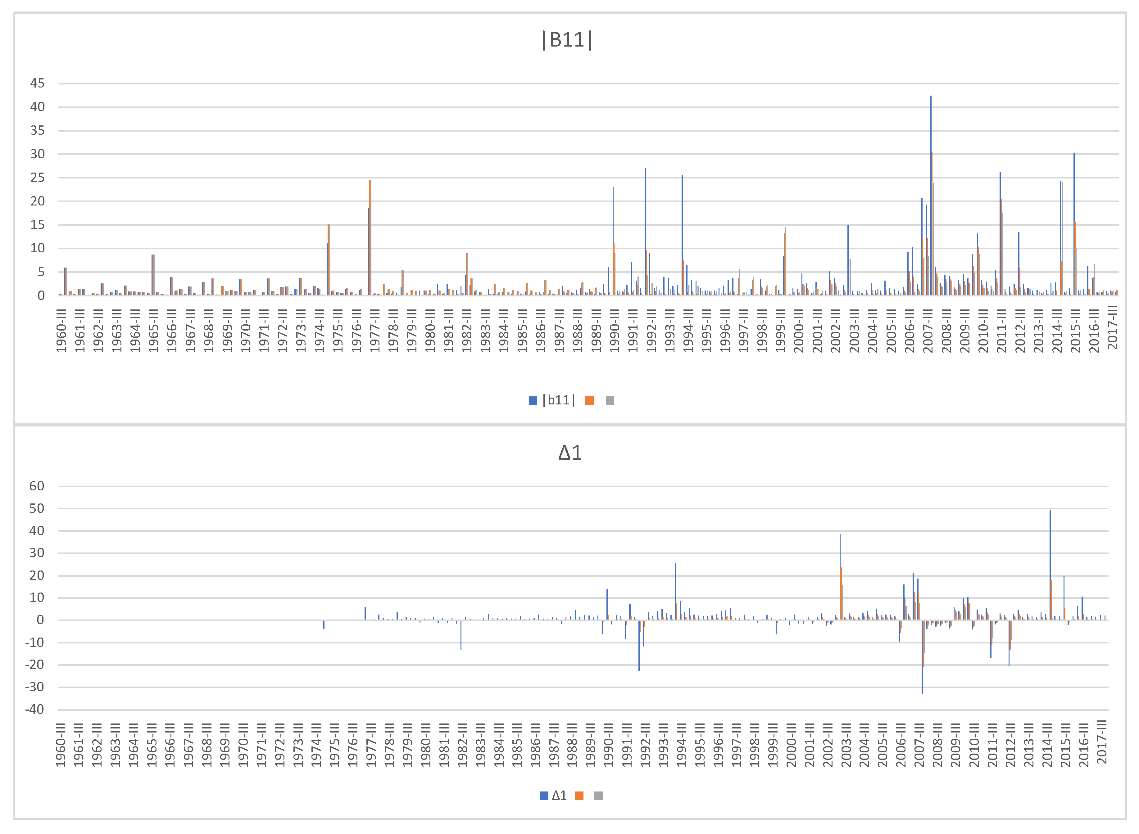
Figure 3 shows the market instability indicator $|b_{11}|$ and default elasticity ${\Delta }_1$ of HNISH from 1960 Q3 to 2017 Q4. The maximum D/W ratio ${\rho }^{\ast }$ is chosen as the three quartiles of the historical D/W ratio from 1960 Q1 to 2017 Q4,6 thus we have three sets of $|b_{11}|$ and ${\Delta }_1$. We can see frequent occurrence of negative ${\Delta }_1$ from 2006 Q3 to 2015 Q4. The Case–Shiller National Home Price Index (SP Dow Jones Indices 2018) recorded a pre-crisis historical peak in 2006 Q2, declined with volatility until 2012 Q1, then started rebounding to reach an all-time high level as of February 2018. The biggest chunk of wealth for ordinary Americans being their homes, it seems justifiable that the decreasing home value implies increasing financial instability. This is indeed true from 2006 Q3 to 2011 Q3, during which not only the real estate market but other invested asset classes experienced heavy loss. In other words, Americans got poorer together during that period. Note that the mathematical threshold that determines financial stability and instability is 1, but as can be seen from the figures below the size of the indicator works as the determinant: the bigger the market instability indicator, the more severe the financial instability.

Now, we divide HNISH into two subgroups, agent r and agent p, using the top 10%–bottom 90% threshold. Let $\alpha$, $\iota$, and $\lambda$ be the wealth, income, and debt share of the poor, respectively. Hence,

$$\begin{array}{cc}\hfill w_p\left(t\right)& =\alpha w_1\left(t\right),\hfill \end{array}$$

(28)

$$\begin{array}{cc}\hfill \sum _{j\ne p}{F}_{pj}\left(t\right)& =\iota \sum _{j\ne 1}{F}_{1j}\left(t\right),\mathrm{and}\hfill \end{array}$$

(29)

$$\begin{array}{cc}\hfill D_p\left(t\right)& =\lambda D_1\left(t\right).\hfill \end{array}$$

(30)

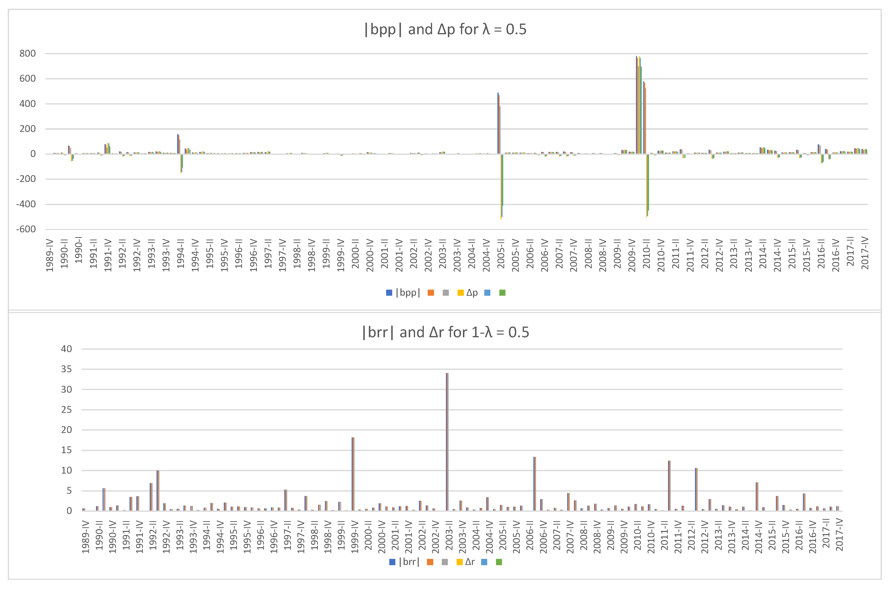
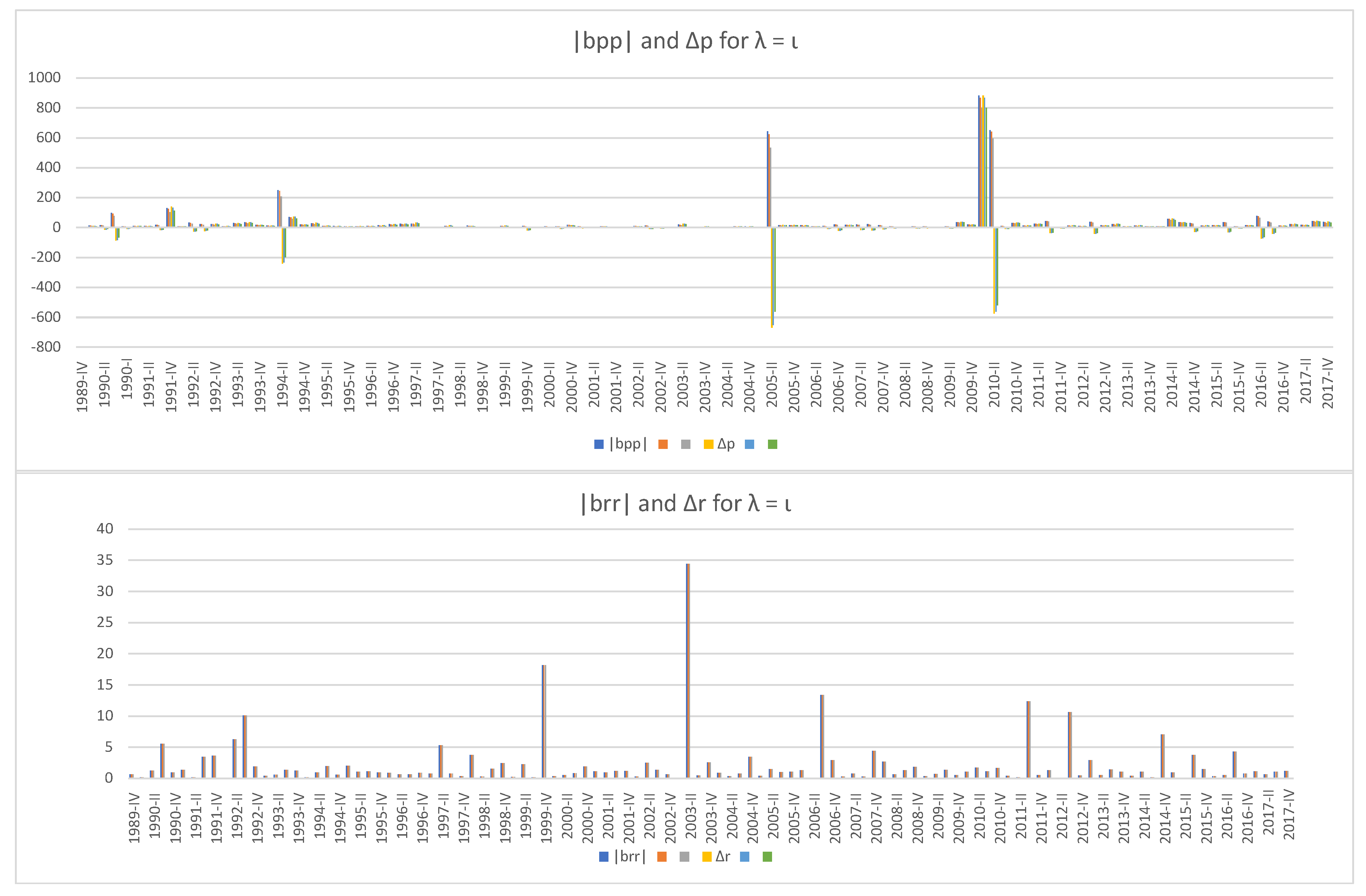
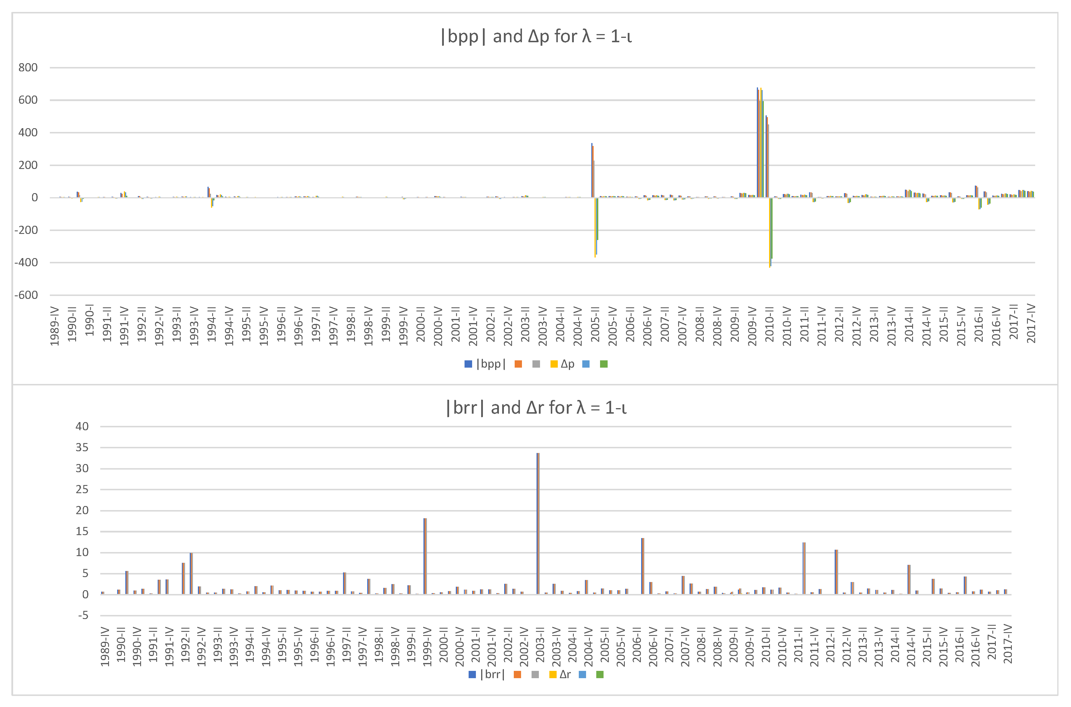
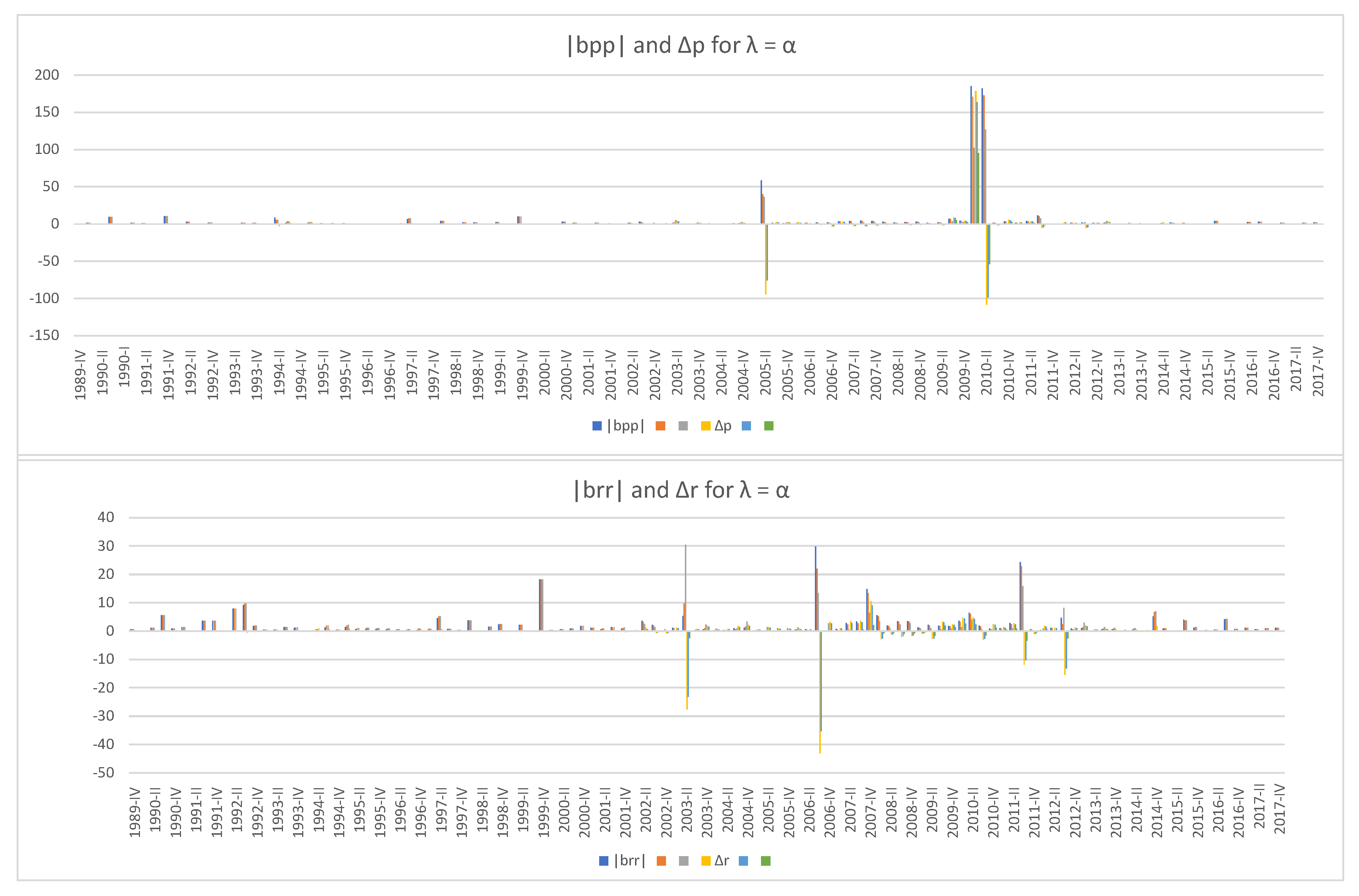
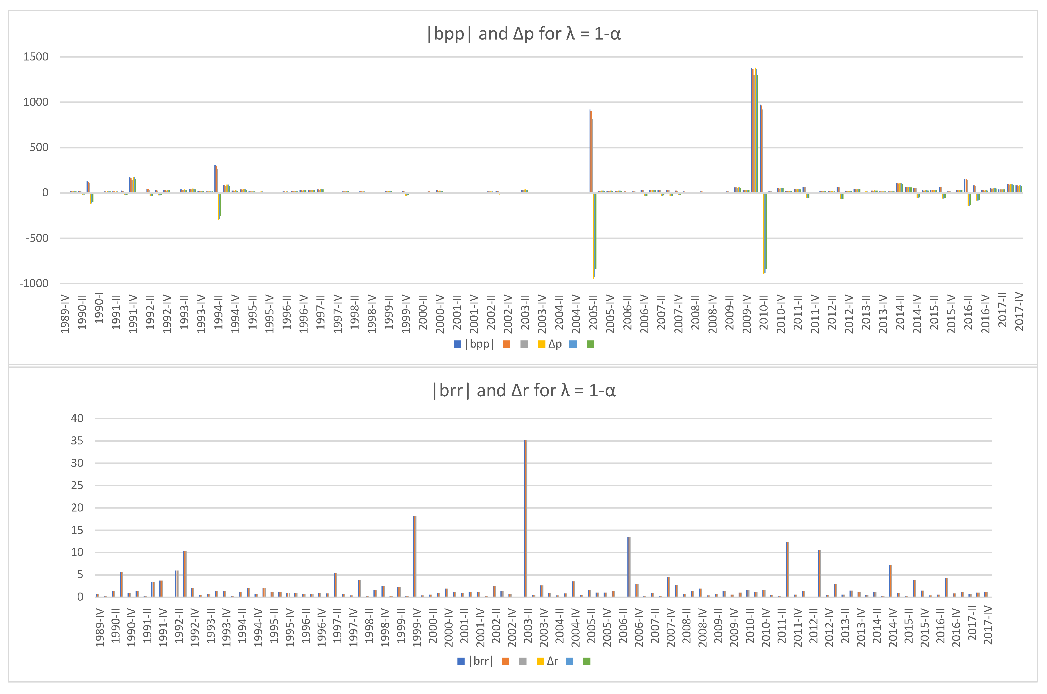
The wealth and income share $\alpha$ and $\iota$ are chosen to suit the 2013–2016 Survey of Consumer Finances, yet the debt share $\lambda$ is not readily available, at least to the author’s knowledge. Hence we consider five cases: $\lambda =0.5$, $\lambda =\iota$, $\lambda =1-\iota$, $\lambda =\alpha$, and $\lambda =1-\alpha$. The last case simulates, in the spirit of Kumhof and Rancière (2010), the scenario in which the poor accumulate debt because their income and wealth do not cover the cost of living. Below are the market instability indicators of the rich and poor subgroups and their default elasticities from 1989 Q4 to 2017 Q4 with ${\rho }^{\ast }$ recalculated for that period. The timeline is chosen to use information from 2013–2016 SCF that goes back to 1989. We can see that the default elasticity ${\Delta }_r$ of the rich becomes negative only when $\lambda =\alpha$, i.e., when their debt share is the same as their wealth share. This case is highly improbable in reality because rich people tend to borrow to invest for higher return, which means they can deleverage at will and never default. Even in that case, the indicators for the rich and the poor rise at different times, $|b_{pp}|$ two years before the 2007–2010 subprime mortgage crisis and at the end of the Great Recession, while $|b_{rr}|$ rises in 2003 amid housing bubbles, in 2006 on the brink of the crisis, and after the Great Recession. In all five cases, the peaks of $b_{pp}$ in 2005 and 2010 are followed by sharp drops in ${\Delta }_p$, while $|b_{rr}|$ rises even when ${\Delta }_r$ remains zero except for the unrealistic case of $\lambda =\alpha$. The rise of $|b_{pp}|$ in late 2009 and early 2010 lasts longer and bigger in magnitude than that in 2005, which suggests that the poor suffered more at the end of the Great Recession than in 2005 when the initially low interest rate of adjustable mortgages were starting to rise, causing a payment spike. Finally, it should be noted that the scale of changes (vertical axes) in $|b_{pp}|$ and ${\Delta }_p$ is far greater than that of their rich counterparts.

When we look at Figure 3, it is 2007 Q3 that seems to be the most financially unstable period during the past three decades, but Figure 4, Figure 5, Figure 6, Figure 7 and Figure 8 tell a different story—that 2007 Q3 was relatively stable, the end of the Great Recession was the worst time for the poor while the rich have been well all the time. It should be mentioned again that, unlike the wealth and income share that are based on real data, the five levels of debt share $\lambda$ are randomly chosen because data on debt distribution could not be found, but they represent diverse debt shares and some of them would decently simulate the reality. The behaviors of the three market instability indicators, $|b_1|$, $|b_{rr}|$, and $|b_{pp}|$ with those selections confirm our conjecture that wealth inequality can create an illusion of financial stability by masking financial instabilities hidden underneath.

5. Conclusions

We have studied masked financial instabilities that are caused by uneven distribution of wealth. When an economic sector is divided into two subsectors that demonstrate a severe wealth inequality, the sector in entirety can appear financially stable while the two subsectors possess respective financial instabilities of opposite nature, one from too much money and the other lack thereof because the wealth of the rich subsector offsets the debt of the poor one to expand the aggregate borrowing capacity of the sector in entirety. The theoretical proposition has been verified by historical macroeconomic time series of the United States households and nonprofit institutions serving households from 1989 Q4 to 2017 Q4 with the income and wealth distribution suggested by the Survey of Consumer Finances (2017) and five different levels of debt chosen by the author. This choice of debt distribution is due to lack of data. Efforts to measure income and wealth concentration go back to a century or so, and there are several established methods to measure the share of top income and wealth group (e.g., Bricker et al. 2015). However, there have not been enough studies on debt in the same spirit as those on wealth distribution. Instead, much emphasis has been made on the measurement of aggregate debt, such as outstanding balance or percentage of wealth. According to Choi (2018), borrowing capacity is a crucial factor in quantifying the level of financial instability. Borrowing capacity being directly related to debt and wealth, correct assessment of debt distribution within an economic sector would give an accurate estimation of both subsectoral and sectoral financial stability. As such, establishing methods to measure the concentration of debt is the goal of our next research.

The United States economy seems to have completely recovered from the Great Recession and be doing better than ever, yet there are factors that could distress part of the economy—those frequently mentioned in the media include high unemployment and stagnant wages for unskilled workers, historically high consumer debt (Federal Reserve Bank of New York 2018) including a dangerously high level of student loans (Foroohar 2017), increasing health care cost, and corporations’ preference for stock buybacks over investment (Phillips and Tankersley 2018). These could exacerbate the wealth inequality in households and make the scenario in Section 3 happen. An uneven distribution of wealth is a frequently discussed issue these days. We believe the topic of this research is timely, and hope that it contributes to calling attention to the part of economy veiled behind benign numbers.

References

- Alawode, Abayomi A., and Mohammed Al Sadek. 2008. What is Financial Stability? Financial Stability Paper Series (1). Available online: http://www.cbb.gov.bh/assets/FSP/What%20is%20Financial%20Stability.pdf (accessed on 18 June 2018).
- Akerlof, George A. 1970. The market for “lemons”: Quality uncertainty and the market mechanism. The Quarterly Journal of Economics 84: 488–500. [Google Scholar] [CrossRef]
- Atkinson, Anthony B., and Salvatore Morelli. 2011. Economic Crisis and Inequality. Human Development Research Paper 2011/06 (06). Available online: http://hdr.undp.org/sites/default/files/hdrp_2011_06.pdf (accessed on 18 June 2018).
- Bernanke, Ben S., Mark Gertler, and Simon Gilchrist. 1999. The financial accelerator in a quantitative business cycle framework. In Handbook of Macroeconomics, Part C. Edited by J. B. Taylor and M. Woodford. Amsterdam: North Holland, vol. 1, pp. 1341–93. ISBN 978-0-444-50158-5. [Google Scholar]
- Bloomberg. 2018. Available online: https://www.bloomberg.com/ (accessed on 18 June 2018).
- Bordo, Michael D., and Christopher M. Meissner. 2012. Does Inequality Lead to a Financial Crisis? NBER Working Paper Series (17896). Available online: http://www.nber.org/papers/w17896 (accessed on 18 June 2018).
- Bricker, Jesse, Alice M. Henriques, Jake A. Krimmel, and John E. Sabelhaus. 2015. Measuring Income and Wealth at the Top Using Administrative And Survey Data; Finance and Economics Discussion Series, 2015-030; Washington, DC: Divisions of Research & Statistics and Monetary Affairs, Federal Reserve Board. [CrossRef]
- Bureau of Labor Statistics. 2018. Labor Force Statistics from the Current Population Survey. Available online: https://data.bls.gov/timeseries/LNS14000000 (accessed on 4 May 2018).
- Carroll, Christopher, Jiri Slacalek, Kiichi Tokuoka, and Matthew N. White. 2017. The distribution of wealth and the marginal propensity to consume. Quantitative Economics 8: 977–1020. [Google Scholar] [CrossRef]
- Castellacci, Giuseppe, and Youngna Choi. 2014. Financial instability contagion: A dynamical systems approach. Quantitative Finance 14: 1243–55. [Google Scholar] [CrossRef]
- Chandra, Sho, and Vince Golle. 2018. The U.S. Economy Has Hit a Milestone. Bloomberg. Available online: https://www.bloomberg.com/news/articles/2018-05-01/as-u-s-expansion-hits-endurance-milestone-here-s-what-s-next (accessed on 18 June 2018).
- Choi, Youngna. 2018. Borrowing Capacity, Financial Instability, and Contagion: Case Study of the U.S. Subprime Mortgage Crisis. Available online: https://papers.ssrn.com/sol3/papers.cfm?abstractid=3013007 (accessed on 30 April 2018).
- Choi, Youngna, and Raphael Douady. 2012. Financial crisis dynamics: Attempt to define a market instability indicator. Quantitative Finance 12: 1351–65. [Google Scholar] [CrossRef]
- Choi, Youngna, and Raphael Douady. 2013. Financial crisis and contagion: A dynamical systems approach. In Handbook on Systemic Risk. Edited by Jean-Pierre Fouque and Joseph A. Langsam. Cambridge: Cambridge University Press, pp. 453–79. ISBN 978-1-107-02343-7. [Google Scholar]
- Congressional Budget Office. 2016. Trends in Family Wealth, 1989 to 2013. Available online: https://www.cbo.gov/publication/51846 (accessed on 30 April 2018).
- Federal Reserve Bank of New York. 2018. Quarterly Report on Household Debt and Credit: 2017 Q4. Available online: https://www.newyorkfed.org/medialibrary/interactives/householdcredit/data/pdf/HHDC_2017Q4.pdf (accessed on 4 May 2018).
- Foroohar, Rana. 2017. The US College Debt Bubble is Becoming Dangerous. The Financial Times. Available online: https://www.ft.com/content/a272ee4c-1b83-11e7-bcac-6d03d067f81f (accessed on 30 April 2018).
- Freixas, Xavier, Luc Laeven, and José-Luis Peydró. 2015. Systemic Risk, Crises, and Macroprudential Regulation. Cambridge and London: The MIT Press, ISBN 978-0-262-02869-1. [Google Scholar]
- Hart, Oliver, and John Moore. 1998. Default and renegotiation: A dynamic model of debt. The Quarterly Journal of Economics 113: 1–41. [Google Scholar] [CrossRef]
- Integrated Macroeconomic Accounts for the United States. 2018. Available online: https://www.bea.gov/national/nipaweb/Ni_FedBeaSna/Index.asp (accessed on 30 April 2018).
- Kochhar, Rakesh, and Anthony Cilluffo. 2017. How Wealth Inequality Has Changed in the U.S. Since the Great Recession by rAce, Ethnicity and Income. Pew Research Center. Available online: http://www.pewresearch.org/fact-tank/2017/11/01/how-wealth-inequality-has-changed-in-the-u-s-since-the-great-recession-by-race-ethnicity-and-income/ (accessed on 30 April 2018).
- Kumhof, Michael, and Romain Rancière. 2010. Inequality, Leverage and Crises. IMF Working Paper 10(268). Available online: https://www.imf.org/external/pubs/ft/wp/2010/wp10268.pdf (accessed on 18 June 2018).
- Organization for Economic Cooperation and Development. 2016. Income Inequality Update. Available online: https://www.oecd.org/social/OECD2016-Income-Inequality-Update.pdf (accessed on 30 April 2018).
- Phillips, Matt, and Jim Tankersley. 2018. Investment Boom from Trump’s Tax cUt Has Yet to Appear. The New York Times. Available online: https://www.nytimes.com/2018/04/30/business/the-tax-cut-buybacks-business-investment.html (accessed on 4 May 2018).
- Piketty, Thomas. 2014. Capital in the Twenty-First Century. Cambridge and London: Belknap Press: An Imprint of Harvard University Press, ISBN 978-0-674-43000-6. [Google Scholar]
- Rajan, Raghuram. 2010. Fault Lines. Princeton: Princeton University Press, ISBN 978-0-691-14683-6. [Google Scholar]
- Saez, Emmanuel, and Gabriel Zucman. 2016. Wealth inequality in the United States since 1913: Evidence from capitalized income tax data. Quarterly Journal of Economics 131: 519–78. [Google Scholar] [CrossRef]
- S&P Dow Jones Indices. 2018. S&P Corelogic Case-Shiller U.S. National Home Price NSA Index. Available online: http://us.spindices.com/indices/real-estate/sp-corelogic-case-shiller-us-national-home-price-nsa-index (accessed on 30 April 2018).
- Survey of Consumer Finances. 2017. Changes in the U.S. Family Finances from 2013 to 2016: Evidence from the Survey of Consumer Finances. Federal Reserve Bulletin 103(3). Available online: https://www.federalreserve.gov/publications/files/scf17.pdf (accessed on 30 April 2018).
- Wolff, Edward N. 2014. Household Wealth Trends in the United States, 1962–2013: What Happened Over the Great Recession? NBER Working Paper (20733). Available online: http://www.nber.org/papers/w20733 (accessed on 30 April 2018).