1. Introduction
In the last few years, there has been a growing interest on minimizing the ruin probability or maximizing the survival probability of the insurance company. An insurance company has to control its ruin probability and keep it at a minimum level to sustain its existence.
Current research on ruin probability has been particularly focused on minimizing the ruin probability. Various methods, such as reinsurance arrangement, dividend payment or investment technique, to minimize the ruin probability have been proposed. However, most of the literature on minimizing the ruin probability is based on the reinsurance arrangements. One of the first examples of optimal reinsurance is suggested by De Finetti [
1]. In that paper, De Finetti determines the optimal retention level for a non-life insurance portfolio under the minimum variance of the insurer’s profit for a fixed expected profit constraint. De Finetti [
1] indicates that the retention level is proportional to the insurance loading factor and inversely proportional to the variance of the risk. Buhlmann [
2] provides further details and proofs of De Finetti’s approach. Borch [
3] shows that the stop loss-reinsurance is the optimal reinsurance contract since it minimizes the variance of the insurer’s risk when the reinsurance premium is calculated by using the expected value premium principles. Arrow [
4] shows that the same stop-loss reinsurance maximizes the expected utility of the terminal wealth of the insurer. Dickson and Waters [
5] use ruin probability instead of the variance criterion in De Finetti’s approach. They investigate the optimal reinsurance levels which minimize the finite time ruin probability for both discrete and continuous time in a non-life insurance portfolio. They assume that the aggregate claims process is approximated by a translated gamma process. Ignatov et al. [
6] explain the optimality as the levels that maximize the joint survival probability for the finite time horizon of the cedent and the reinsurer. They derive a formula for the expected profit under the probability of survival of the insurer. Kaluszka [
7] proposes the optimal reinsurance which minimizes the ruin probability for the truncated stop loss reinsurance based on different pricing rules, such as the economic principle, generalized zero-utility principle, Esscher principle and mean-variance principle. Dickson and Waters [
8] focus on a dynamic reinsurance strategy to minimize the ruin probability. They derive a formula for the finite time ruin probability for discrete and continuous time by using the Bellman optimality principle. Moreover, they show how the optimal strategies are determined by approximating the compound Poisson aggregate claims distributions by translated gamma distributions and by approximating the compound Poisson process by a translated gamma process, respectively. Kaishev and Dimitrova [
9] generalize a joint survival optimal reinsurance model for the excess of loss reinsurance under the assumption that the individual claim amounts are modeled by continuous dependent random variables with a joint distribution. The optimal retention levels that maximize both the joint survival function and the premium income are determined. Nie et al. [
10] propose a new kind of reinsurance arrangement, for which the reinsurer’s payments are bounded above by a fixed level. In this reinsurance type, whenever the insurer’s surplus falls between zero and this fixed level, the reinsurance company makes an additional payment called capital injections. The optimal pair of initial surplus and the fixed reinsurance level is determined to make the ultimate ruin probability minimum. Centeno [
11], Aase [
12], Ignatov et al. [
6], Balbas et al. [
13] and Centeno and Simoes [
14] summarize the research techniques that are used in optimal reinsurance and provide further references about optimal reinsurance studies.
Briefly, the findings of these studies indicate that optimal reinsurance levels are mostly determined by using a single criterion (e.g., minimizing a ruin probability). Furthermore, there are few studies in the literature that focus on determining the optimal reinsurance level under different constraints. Dimitrova and Kaishev [
15] and Hürlimann [
16] have studied optimal reinsurance by considering different risks from the point of both the insurer and the reinsurer.
Karageyik and Dickson [
17] suggest optimal reinsurance criteria as the released capital, expected profit and expected utility of resulting wealth. They aim to find the pair of initial surplus and reinsurance level that maximizes the output of these three quantities under the minimum finite time ruin probability by using the translated gamma process to approximate the compound Poisson process. In order to obtain the optimal reinsurance, they take the advantage of the decision theory and use the TOPSIS method with the Mahalanobis distance. Based on the approach introduced in Karageyik and Dickson [
17], the purpose of this paper is to determine the optimal initial surplus and retention level that maximize the optimal reinsurance criteria under the minimum ultimate ruin probability constraint.
Different from Karageyik and Dickson [
17], we investigate the optimal reinsurance level by using three utility functions: exponential, fractional and logarithmic, besides the expected profit and released capital criteria. Although, Karageyik and Dickson [
17] examine optimal reinsurance under the finite time ruin probability, we prefer to use the ultimate ruin probability constraint. In addition, we use two multi-attribute decision making methods: AHP and TOPSIS with four normalization and two distance measure techniques in the decision analysis part. We have obtained and compared the optimal initial surplus and retention level for the combinations of different loading factors.
The rest of the paper is structured as follows:
Section 2 describes the classical risk model.
Section 3 briefly introduces the ultimate ruin probability under the assumption of the aggregate claims amount approximated by the translated gamma process.
Section 4 explains the optimal reinsurance criteria: released capital, expected profit, exponential, fractional and logarithmic utility functions.
Section 5 presents two multi-attribute decision making methods: AHP and TOPSIS.
Section 6 focuses on the application to determine the optimal initial surplus and retention level for the exponential and Pareto claims.
Section 7 concludes the paper.
2. Classical Risk Model
The insurer’s surplus process at time
t,
, is:
where
is the initial surplus,
c is the constant premium rate with
and
is the aggregate claim amounts up to time
t.
The aggregate claim amount up to time
t,
, is:
where
denotes the number of claims that occur in the fixed time interval
. In the classical risk model, it is assumed that
is a Poisson process with parameter
λ. The individual claim amounts are modeled as independent and identically distributed (i.i.d) random variables
with distribution function
, such that
, and
is the amount of the
i-th claim. The density function and the
k-th moment of
are represented as
f and
.
The infinite time ruin probability in the continuous case (ultimate ruin probability) is defined as:
defines the probability that the insurer’s surplus falls below zero at some time in the future, that is claims outgo exceed the initial surplus plus premium income. It is usually assumed that the premium income is greater than the expected aggregate claim amount per unit of time
. Otherwise,
for all
.
Trufin et al. [
18] deal with the infinite time ruin probability of an insurance portfolio in the framework of risk measures. They also point to the advantages of the infinite time approach over the finite time case. They indicate that there are no difficulties of planning and assuming the appropriate operational time in the infinite time analysis contrary to the finite time case.
In this study, the expected value premium principle is applied with the formula where θ is the insurance loading factor with .
Under an excess of loss reinsurance arrangement, the insurer and the reinsurer’s expected individual claim amounts are calculated according to a constant retention level
M. When a claim
X occurs, the insurer pays
, and the reinsurer pays
with
. Hence, the distribution function of
Y,
, is:
and the moments of
Y are:
Similarly, the moments of
Z are:
The expected aggregate claim amount, denoted by
, is calculated by the expected number of claims and the expected amount of each claim as:
The aggregate claim amount is shared by the insurance and reinsurance company irrespective of the type of reinsurance arrangement; the aggregate claim amount S can be written as , which denotes the insurer’s net aggregate claims after the reinsurance arrangement, and denotes the reinsurer’s aggregate claim amount. , the expected total claim amount paid by the reinsurer, is calculated as , whereas the net of expected claim amount paid by the insurer, is calculated as .
According to the expected value premium principle with the insurance loading factor
θ and the reinsurance loading factor
ξ, the insurer’s premium income per unit time after the reinsurance premium (i.e., net of reinsurance) is defined as:
where we assume that
and
(see Dickson [
19]).
6. Numerical Analysis
In this section, we present some numerical examples on determining the optimal initial surplus and retention level under the minimum ultimate ruin probability and maximum reinsurance criteria. We make the following assumptions: the individual claim amount has an exponential distribution with a probability density function and Pareto distribution with a probability density function with and . The number of claims per unit time has a Poisson distribution with the parameter ; the premium loading factors combinations are (θ, ξ), numerically , , and .
Individual claim amounts are assumed to have the exponential and Pareto distributions, which have different tail structures. Pareto is a heavy-tailed distribution, which is essential for modeling extreme losses, whereas exponential is a light tailed distribution. Hence, we can investigate the effects of different individual claim distributions on optimal values. The expectations of the aggregate claims are the same; however, the variances are different.
A set of alternatives which consists of initial surplus and retention level pairs is calculated under the ultimate ruin probability constraint. The insurer’s released capital, expected profit, exponential, logarithmic and fractional expected utilities are calculated by using these pairs. In the decision analysis part, we use both the AHP and TOPSIS method to select the optimal initial surplus and reinsurance level. The algorithm for the excess of loss reinsurance can be summarized as follows.
Step 1: Calculation of the ultimate ruin probability under the translated gamma process approximation:
In the calculation of the ultimate time ruin probability, we obtain the parameters of the translated gamma process and the loading factor,
, by using (
7) and (
11), respectively. Then, we use this loading factor in the calculation of the probability of ruin under the standardized gamma process with the premium loading factor
being
, with
defined in (
8).
Step 2: Calculation of the largest initial surplus under the minimum ultimate ruin probability:
The largest initial surplus is obtained from (
8), such that this probability equals 0.01. The largest initial surplus depends only on
θ, since the reinsurance is not involved in this case. When the individual claim has an exponential and Pareto distribution, the largest initial surpluses, which are calculated according to two different insurance loading factors
and
, are given in
Table 4.
The results show that when the individual claim amount has a Pareto distribution, the required largest initial surplus is higher than in the exponential case.
Step 3: Calculation of the smallest initial surplus under the minimum ultimate ruin probability:
When the reinsurance arrangement is involved, moments of the insurer’s net individual claims are calculated for the exponential claims by using (
12) and for the Pareto claims by using (
13)–(
15). Then, the parameters of the translated gamma process are calculated according to (
7). Hence, by using these parameters, the loading factor
is calculated by (
11), and then, we integrate this loading factor into (
8). The smallest initial surplus that makes the ruin probability equal to 0.01 is calculated by using the one-dimensional optimization technique, which searches the interval from lower to upper for a minimum or maximum value of (
8) in
R programming. The corresponding retention levels
M of the smallest initial surplus are calculated.
In the calculation of the smallest initial surplus
and the corresponding retention level
M, four different premium loading factors (
θ,
ξ) are used: (0.1, 0.15), (0.1, 0.2), (0.1, 0.3) and (0.2, 0.3). These loading factors are the same as in Dickson and Waters [
25]. The smallest initial surpluses under the excess of loss reinsurance are given in
Table 5. These smallest initial surpluses are used as the starting points of the alternative set.
As seen in
Table 5, the required smallest initial surplus for the Pareto claims is higher than in the exponential case. The same situation is observed for the largest initial surplus.
Step 4: Constitution of the alternative set that consists of the pair of initial surplus and retention level:
We design a set of alternatives that consist of the pair of initial surplus and retention level. We begin with the smallest initial values and increase this value by 0.1 or 0.05 to the largest initial surplus . Then, we calculate the corresponding retention level for each initial surplus. Hence, we obtain an outcome set that presents all of the possible combinations of the retention level and the corresponding initial surplus. Each pair of outcome sets is denoted as .
Step 5: Calculation of the optimal reinsurance criteria according to the initial surplus and the retention level:
The set of
is used in the calculation of the optimal reinsurance criteria. The released capital is calculated as
; the expected profit is calculated by (
16); and expected utilities are calculated by (
17)–(
19), respectively. For the calculation of expected profit, the parameters of the translated gamma process
α,
β and
k are needed. These parameters are calculated according to the retention level,
M. However, in the calculation of the expected utility, not only the retention level, but also the initial surplus
is needed.
Table 6 and
Table 7 illustrate each alternative initial surplus and retention level pair with their corresponding optimal reinsurance criteria for four different loading combinations under the exponential and Pareto claim case, respectively.
The analysis indicates that because of the high variance of the Pareto distribution, the differences between the starting point (smallest initial surplus) and the ending point (largest initial surplus) under each criterion are higher than those in the exponential claims case. In particular, we can see a huge range in the expected profit and released capital by comparing with the exponential claims.
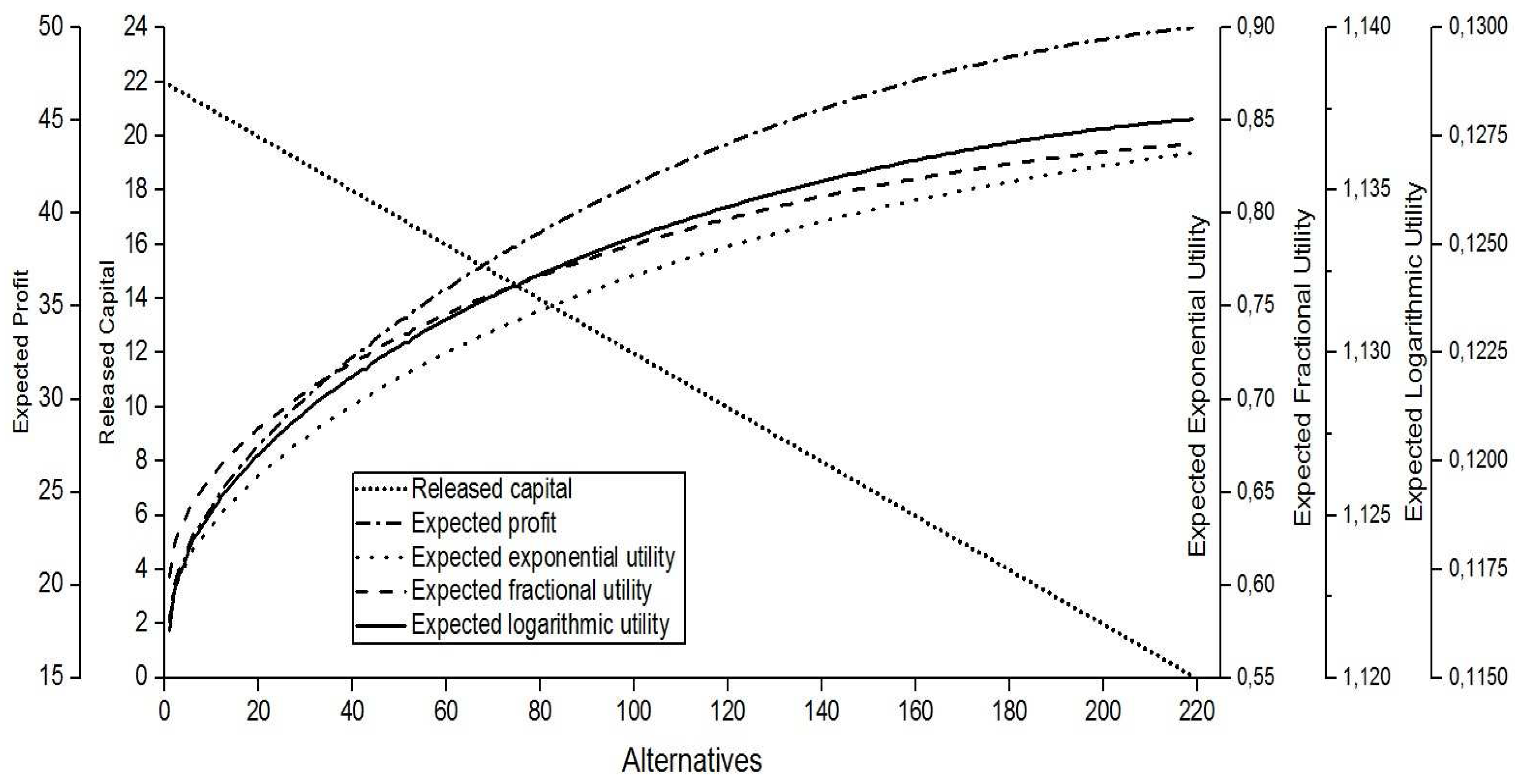
Figure 1 shows the behavior of five criteria when
and
for the exponential claims under the excess of loss reinsurance. The
x-axis of this graph shows the number of the alternatives for the pair
, while the results of the five criteria appear on the
y-axis. We prefer to use a plot with five
y-axes and one shared
x-axis because of the different scales.
We can see that each criterion has a different pattern. In the excess of loss reinsurance, as the initial surplus increases, the corresponding retention level also increases in order to get a fixed ruin probability, such as 0.01. When the pair increases, the released capital decreases. However, both the expected profit and the expected utility functions increase with different slopes.
It can be clearly seen that the released capital declines steadily to the level of zero as the initial surplus closes to . The expected profit increases with a decreasing slope. The first alternative begins with the maximum released capital and the minimum expected profit and minimum expected utility. Conversely, the last alternative has the maximum expected profit and expected utility and the minimum released capital.
Step 6: Decision of the optimal pair of initial surplus and retention level under the AHP and TOPSIS methods:
In order to decide the optimal pair of initial surplus and retention level , we use the AHP and TOPSIS methods with four normalization and two distance measure techniques. In the TOPSIS method, we use the Euclidean and Mahalanobis distances. In the TOPSIS method with the Mahalanobis distance, we investigate the relationship between the criteria by using the vector-normalized covariance matrix. The relative proximity to the ideal solution for each alternative is used in deciding the optimal pairs . In the decision process, it is required to state how criteria or alternatives affect each other. In our study, five criteria have different scales and maximum/minimum levels.
In order to obtain a comparable scaled values and pairwise comparisons matrix, we use four different normalization techniques: AHP-1, AHP-2, AHP-3 and AHP-4.
- AHP-1
uses the linear scale transformation normalization technique. The normalized values are obtained by dividing the outcome of a criterion by its maximum value. Then, we assume that the maximum normalized value of the criterion is equal to nine as in Saaty’s matrix (
Table 2) (Hwang and Yoon [
28]). Thus, the scale of measurement varies precisely from 1–9 for each criterion.
- AHP-2
uses the vector normalization technique as used in the TOPSIS method in (
20).
- AHP-3
uses the min-max normalization technique, which is given below:
- AHP-4
uses the automating pairwise comparison technique [
32]. In this technique, a pairwise comparison matrix
is comprised of the m criteria,
. The matrix
is a
real matrix, where
n is the number of alternatives. Each element
of the matrix
represents the evaluation of the
-th alternative compared to the
-th alternative with respect to the
-th criterion.
The
-th criterion changes in the interval
, and
and
are the attributes under the
-th and
-th control options. When
, the analogous value
of
can be computed as:
When
, the analogous value
of
can be computed as:
The key limitation of this technique is the assumption of a linear relationship between the difference of and .
The variance of the outcomes has an important role in the determination of the optimal levels in the TOPSIS method. The covariance matrix of the vector-normalized outcomes when and is obtained as:
Since the variance and covariance values of the expected utility criteria are small, the expected utility criteria seem to be more ineffectual criteria than the others. However, the variance of a set of outcomes for the released capital is higher than the variance of the corresponding outcomes for other criteria, so it has a dominant impact on decision making. Firstly, we calculate the optimal initial surplus and retention level assuming that five criteria have the same importance. Then, we observe the changes in the optimal pairs by modifying the weight of the released capital in the range from 0–1.
Table 8 presents the optimal initial surplus and retention level for the exponential and Pareto claims with four different loading combinations under two TOPSIS and four AHP methods. In this calculation, it is assumed that equal weights are allocated to each criterion, such as 1/5. From this table, it can be seen that the optimal pairs in the Pareto case are higher than in the exponential case for all methods. In addition, the optimal levels increase when the reinsurance loading factors increase, since the higher reinsurance premium causes a decrease on the expected profit. Based on the results, the following conclusions can be drawn. First, the results show that the distance measure has a vital role in optimality. The TOPSIS method with the Mahalanobis distance gives smaller optimal pairs than the TOPSIS method with the Euclidean distance. The most likely explanation for this situation is the effect of dependency between the criteria. When the criteria are affected by each other, there will be some changes on the optimal pairs. Hence, we can see that the TOPSIS method with the Mahalanobis distance gives more accurate and conservative results than the Euclidean case.
Second,
Table 8 shows that the normalization technique plays an important role in optimality. AHP-1, AHP-2 and AHP-4 give slightly different optimal results than the TOPSIS method, whereas AHP-3 provides quite different optimal levels than the other methods. The underlying reason for this discrepancy is the normalization technique. AHP-3 depends on the normalization technique, which is calculated as dividing
by
. The denominator gives the range of the set of data, the difference between the highest and lowest values in the set. The range of the released capital is the highest among the other criteria. In addition, the numerator leads with zero in the starting point of the expected profit and expected utility since the starting point of these criteria are equal to their minimum values. Hence, the normalized values of each criteria except the released capital criterion are increasing towards the last points of the set of alternatives. Therefore, optimal levels that are closer to the no-reinsurance case (high initial surplus and high retention level) are determined as the optimal strategy.
The AHP-4 method produces very close optimal results to the TOPSIS methods since the pairwise comparison techniques are used. This normalization technique is efficient especially when the difference between alternatives is based on a linear structure. In our analysis, since each alternative has a linear form, this normalization technique is more suitable than the other normalization techniques.
In order to verify the validity of the optimal pairs, we carry out different scenarios. We check for the presence of the criteria weights on the optimal pairs. We observe the changes on the optimal levels when the weight of the released capital varies between zero and one. We choose the released capital since it has the highest variance compared with other criteria. The equal weight assumption does not enable us to compare the optimal results visually because of the small variance of the expected utility. Therefore, we assume that the weight of the expected profit equals the summation of the weight of the expected utility criterion.
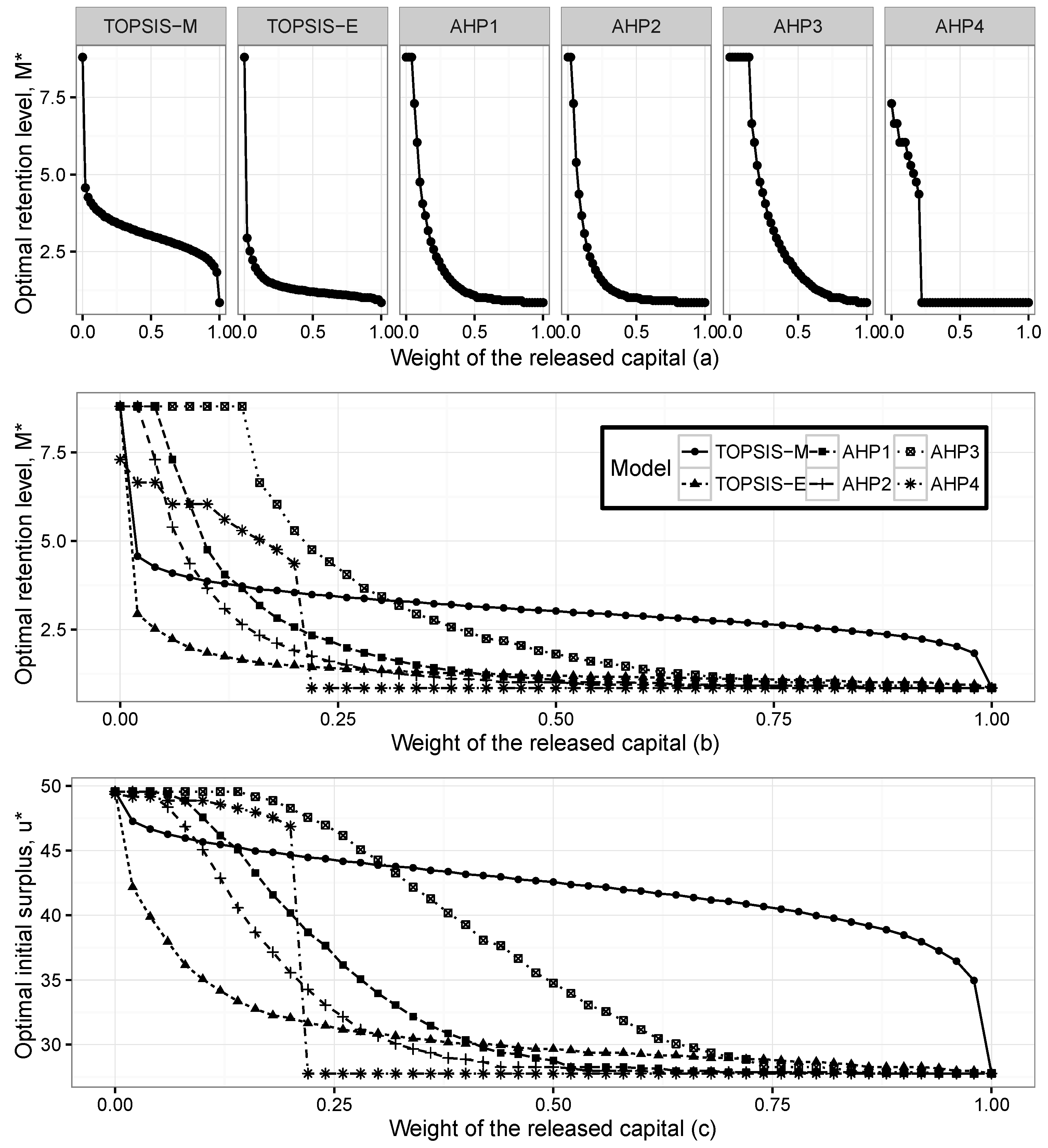
Figure 2 presents the optimal initial surplus
and optimal retention level
, for the exponential claims when the weight of the released capital changes between zero and one.
Figure 2a presents the optimal retention levels for six methods separately. The optimal levels are obtained as the maximum point of the closeness index in the TOPSIS method and the priority index in the AHP method. When the weight of the released capital increases, the optimal levels get closer to the point where the released capital is maximum. When the weight of the released capital is zero, the optimal levels are obtained at the maximum points of the expected profit and expected utility. It can be clearly seen that the shapes of the optimal levels are different for each method. The significant limitation exists in AHP-4, after the level where each criterion has the same importance, the optimal retention levels are obtained at the points where the released capital has its maximum level.
Figure 2b presents changes in the optimal retention levels according to six methods in the same scale, whereas
Figure 2c shows the changes in the optimal initial surplus.
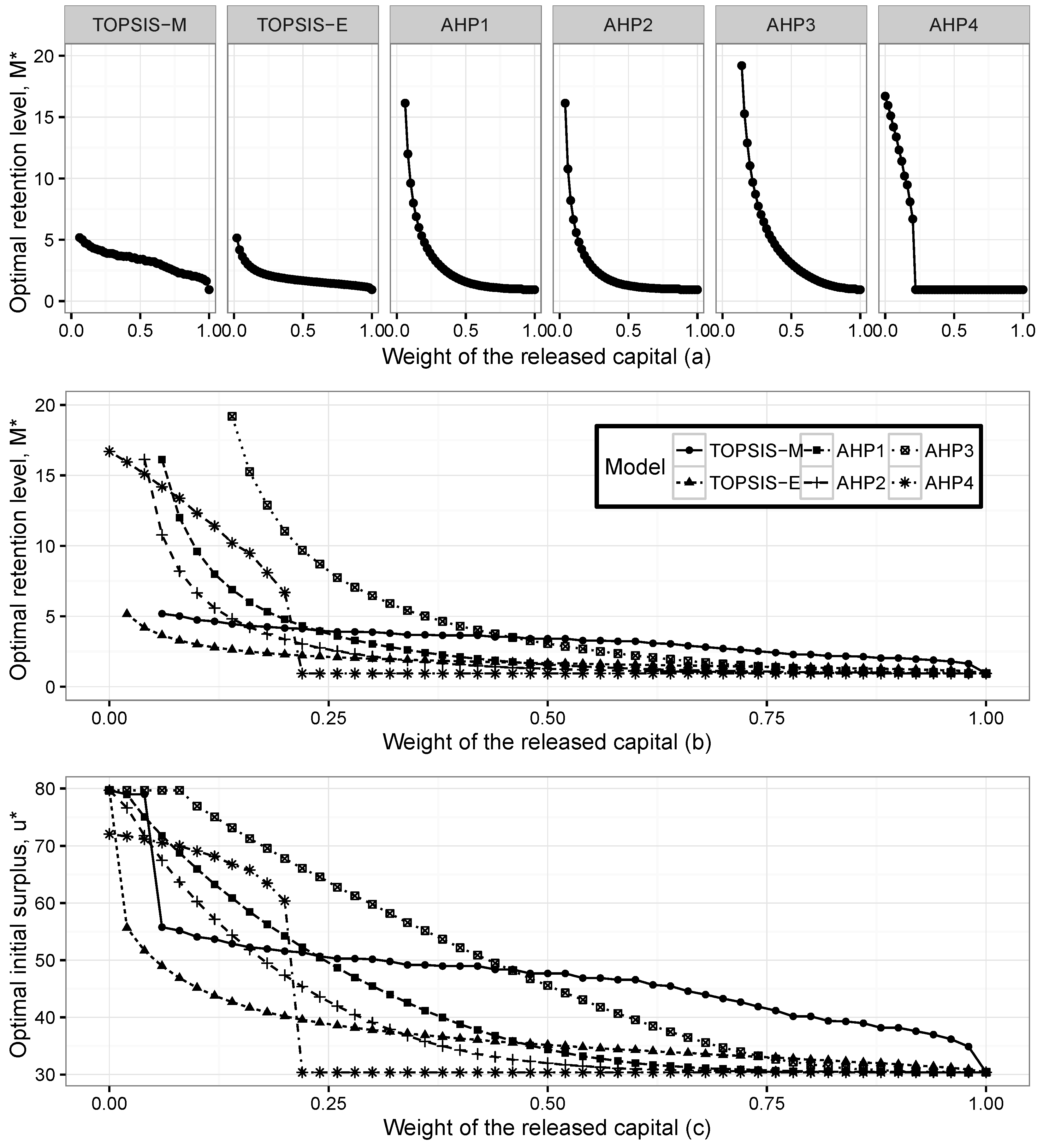
Figure 3 presents the optimal initial surplus
and optimal retention level
for the Pareto claims when the weight of the released capital changes between zero and one.
It is seen that Pareto and the exponential distributions give compatible results. We can observe that when the weight of the released capital increases, the optimal pairs go towards the level where the released capital has its maximum. The pattern of the optimal levels does not change for both individual claim assumptions; however, the range of the optimal pairs in Pareto claims is wider than in the exponential case.
However, as can be seen from both figures, the TOPSIS method with the Mahalanobis distance gives different optimal pairs compared to the other methods. The results show that the dependency has a significant effect on the determination of optimal reinsurance levels. In order to verify our method, we compare optimal pairs according to the changes on the weights of the expected profit and expected utility functions. These results are consistent with the findings of the released capital case. We can observe that when the weights of the expected profit or expected utility functions increase, the optimal pairs go towards their maximum level, as well.


