
How Does Reinsurance Create Value to an Insurer? A Cost-Benefit Analysis Incorporating Default Risk

Department of Statistics and Actuarial Science, The University of Iowa, 241 Schaeffer Hall, Iowa City, IA 52242-1409, USA
Risks 2016, 4(4), 48; https://doi.org/10.3390/risks4040048
Submission received: 9 October 2016
/
Revised: 5 December 2016
/
Accepted: 7 December 2016
/
Published: 16 December 2016
(This article belongs to the Special Issue Selected Papers from the 6th Gerber-Shiu Workshop and the 3rd Modeling of Heavy-Tail Phenomena Workshop)
Abstract
:Reinsurance is often empirically hailed as a value-adding risk management strategy which an insurer can utilize to achieve various business objectives. In the context of a distortion-risk-measure-based three-party model incorporating a policyholder, insurer and reinsurer, this article formulates explicitly the optimal insurance–reinsurance strategies from the perspective of the insurer. Our analytic solutions are complemented by intuitive but scientifically rigorous explanations on the marginal cost and benefit considerations underlying the optimal insurance–reinsurance decisions. These cost-benefit discussions not only cast light on the economic motivations for an insurer to engage in insurance with the policyholder and in reinsurance with the reinsurer, but also mathematically formalize the value created by reinsurance with respect to stabilizing the loss portfolio and enlarging the underwriting capacity of an insurer. Our model also allows for the reinsurer’s failure to deliver on its promised indemnity when the regulatory capital of the reinsurer is depleted by the reinsured loss. The reduction in the benefits of reinsurance to the insurer as a result of the reinsurer’s default is quantified, and its influence on the optimal insurance–reinsurance policies analyzed.
Keywords:
marginal cost; marginal benefit; distortion; 1-Lipschitz; premium; Value-at-Risk; VaR; TVaR; comonotonicity; counterparty risk1. Introduction
In today’s complex and catastrophe-plagued business environment, the judicious use of risk mitigation strategies in general and reinsurance in particular is vital to the sustainable financial viability of insurance corporations. Being essentially insurance purchased by an insurer from a reinsurer, reinsurance has served as a time-honored risk management activity on which an insurer can capitalize to achieve manifold mutually complementary business objectives. From a risk management perspective, reinsurance provides a powerful tool for an insurer to stabilize its risk exposure by ceding unbearable catastrophic losses to a reinsurer, which is generally more geographically diversified than an insurer. As a result, the amount of risk and the concomitant capital requirement faced by the insurer can be maintained at a level that the insurer deems appropriate. Meanwhile, reinsurance bolsters the underwriting capacity of the insurer and, in turn, empowers the insurer to assume losses from its policyholders that it is otherwise incapable of underwriting. This results in more insurance business opportunities, contributes to the prosperity of the insurance industry and does a service to the society at large. On an accounting front, reinsurance can be utilized to reduce taxes and effect administrative savings as well as surplus relief. These merits of reinsurance have been documented empirically in various sources, such as Cummins et al. [1], Holzheu and Lechner [2], Bernard [3], Tiller and Tiller [4], just to name a few.
In the academic community, research on reinsurance has predominantly centered upon the bilateral contract design problem between the insurer and reinsurer. Initiated in Borch [5] and Arrow [6] involving the variance minimization and expected utility maximization of the terminal wealth of an insurer, and later extended to a risk-measure-theoretic framework, as in Cai et al. [7], Chi and Tan [8], Cui et al. [9] and Lo [10], among others, the study of optimal reinsurance contracts has been investigated with a diversity of objective functionals and premium principles of varying degrees of technical sophistication, with noticeable mathematical contributions having been made. Optimal reinsurance contracts ranging from stop-loss, quota-share policies to general insurance layers have been found depending on the precise specification of the reinsurance model under consideration. Apart from being preoccupied with mathematical advancements with little economic motivation, the majority of existing research work is confined to the bilateral insurer–reinsurer setting with an exogenously fixed reinsurable loss in the first place, and ignores the interaction between the insurer and its primary policyholders. Doing so overlooks the substantive fact that reinsurance does enlarge the underwriting capacity of the insurer, which, in turn, affects the amount of insured loss that can be reinsured. In fact, it is the interplay between insurance and reinsurance that differentiates these two technically indistinguishable but practically distinct activities. To the best of the author’s knowledge, Zhuang et al. [11] were the first to undertake a comprehensive analysis of optimal insurance–reinsurance in the context of a one-period three-party model involving a policyholder, an insurer and a reinsurer. In this model, the insurer has the privilege to decide on not only how much risk to underwrite from the policyholder, but also how much insured loss to cede to the reinsurer in order to achieve minimality of its overall risk. As one may have expected, these two decisions are closely intertwined. It was pointed out in Zhuang et al. [11] that reinsurance enhances the risk taking capacity and profit of an insurer (see Proposition 3.2 therein).
To bridge the existing gap between empirical studies and theoretical research on optimal reinsurance, this article strives to scientifically quantify the value that reinsurance introduces to an insurer on the basis of a variant (see the next paragraph) of Zhuang et al.’s [11] distortion-risk-measure (DRM)-based three-party model, where the policyholder, insurer and reinsurer interact closely. By virtue of the tractable properties of DRM, the optimal insurance–reinsurance problem is completely solved through an explicit joint construction of the optimal insurance and reinsurance policies. Compared with Zhuang et al. [11], our novel contributions include intuitive but mathematically rigorous explanations on the marginal cost and benefit considerations underlying the optimal insurance–reinsurance decisions and the formation of the extra value created by reinsurance. As in Cheung and Lo [12], the integral form of various quantities under the DRM framework will be instrumental in the development of these explanations. Demystifying our explicit optimal solutions, the cost-benefit discussions indicate that the benefits of reinsurance to the insurer are twofold, via the opportunity to cede currently underwritten losses to the reinsurer for a further reduction in the insurer’s overall risk, as well as an improved capability to accept losses from the policyholder in the first place. Analytic expressions accounting for the benefits in these two respects are obtained. The bottom line is that reinsurance furnishes the insurer with a flexible mechanism to lower its cost of transaction. Overall, our results not only conform to empirically supported findings in most reinsurance markets, but also shed valuable light on the economics of insurance and reinsurance, which most existing research contributions are very much lacking in.
Risk transfer inevitably introduces counterparty risk, and reinsurance is no exception. By engaging in a reinsurance contract with the reinsurer, the insurer is exposed to the undesirable possibility that the reinsurer fails to deliver on its promised obligations, which, in turn, jeopardizes the insurer’s ability to indemnify the policyholder in the first place. The default risk of the reinsurer, if not taken into account, may result in the insurer forming an overly optimistic view of its risk exposure and devising an unduly aggressive insurance–reinsurance strategy. Motivated by Asimit et al. [13] and Cai et al. [14], we embed the reinsurer’s default risk in our three-party model by assuming that the reinsurer will default on its obligations whenever the size of the promised reinsured loss exceeds the reinsurer’s regulatory capital, which is prescribed as the Value-at-Risk (VaR) of the reinsured loss. Such a choice of the regulatory capital is commensurate with the riskiness of the reinsured loss and can be explained by the popularity of VaR in the banking and insurance industries as well as the recent implementation of the Solvency II regulatory framework in European Union countries. We also allow for loss recovery by postulating that a fixed portion of the excess of the reinsured loss over the regulatory capital will be paid to the insurer as partial compensation in the case of default. As a by-product, the results in our three-party model are indicative of the repercussions that the reinsurer’s default risk can have for the design of the optimal insurance and reinsurance policies.
The remainder of this article is structured as follows: Section 2 sets forth the DRM-based three-party optimal insurance–reinsurance model subject to default risk, which forms the backbone of the entire article, describes its various components and formulates the risk minimization problem faced by the insurer. In Section 3, the optimal insurance–reinsurance strategies are analytically obtained and intuitively explained from a cost-benefit perspective that informs the value created by reinsurance, and an illustrating numerical example is given. Section 4 concludes the article with some potential future research directions.
2. Three-Party Optimal Insurance–Reinsurance Model with Default Risk
Synthesizing the discussions in Asimit et al. [13] and Zhuang et al. [11], we begin with a precise description of a DRM-based insurance–reinsurance model in which three agents, namely a policyholder, an insurer and a default-prone reinsurer, coexist. In this model, the risk faced by an agent is evaluated by means of distortion risk measures (DRMs), whose definition calls for the notion of a distortion function (see Denneberg [15] and Wang [16]). We say that is a distortion function if g is a non-decreasing function, such that and . Unlike Zhuang et al. [11], no (left- or right-) continuity assumptions are imposed on g, neither are convexity or concavity conditions, because our analysis is valid without these extraneous technical assumptions and therefore holds in high generality, with the agent being at complete liberty to choose a distortion function that best aligns with his/her risk preference. Corresponding to a distortion function g, the DRM of a random variable Y is defined by
where is the survival function of Y, provided that at least one of the two integrals in Formula (1) is finite. For non-negative random variables, Formula (1) reduces to
In this article, we tacitly assume that all random variables are sufficiently integrable in the sense that their DRMs are well-defined and finite.
As a risk quantification vehicle, DRM enjoys a number of practically appealing and mathematically tractable properties, including:
- Translation invariance: If Y is a random variable and c is a real constant, then
- Positive homogeneity: If Y is a random variable and a is a non-negative constant, then
- Comonotonic additivity: If are comonotonic random variables in the sense that they are all non-decreasing functions of a common random variable, then
These properties, which can be found in Equations (52)–(54) of Dhaene et al. [17], will play a vital role in tackling the objective function of the insurer’s risk minimization problem studied in this article. Furthermore, the class of DRM is a big umbrella under which many common risk measures fall, most notably VaR, whose definition is recalled below. In the sequel, we write , and denote the indicator function of a given set A by , i.e., if A is true, and otherwise.
Definition 1.
(Definition of VaR) The Value-at-Risk (VaR) of a random variable Y at the probability level of is the generalized left-continuous inverse of its distribution function at p:
with the convention .
It is known that the distortion function that gives rise to the p-level VaR is (see Equation (4) of Dhaene et al. [17]), which is neither convex nor concave. For more information about the practical use of VaR, readers are referred to the comprehensive guide of Jorion [18].
In the current three-party insurance–reinsurance model, the policyholder, insurer and reinsurer interact as follows. Underlying the entire analysis is the policyholder’s ground-up loss modeled by a non-negative random variable X with a known distribution, which can be underwritten by the insurer via an insurance contract characterized by the insurance indemnity function . The effect of insurance is that the ground-up loss X is partitioned into , the insured loss against which the insurer is obligated to indemnify the policyholder, and , the loss retained by the policyholder. In return for insuring part of the ground-up loss, the insurer receives the insurance premium , which is a function of the insured loss, from the policyholder. At this point, the insurer’s net risk exposure is .
Meanwhile, to mitigate its risk exposure resulting from the insurance contract, the insurer has the opportunity to reinsure part of the insured loss through a reinsurance contract with the reinsurer, which is capable of indemnifying the insurer up to the amount of its regulatory capital in place. Given the recent implementation of the Solvency II regulatory framework in the countries of the European Union, we follow Asimit et al. [13] and assume that the reinsurer operates in a VaR-regulated environment and thus prescribes its regulatory capital in accordance with the β-level VaR of the reinsured loss for some large probability level β (e.g., in Solvency II). If represents the reinsurance indemnity function and is the recovery rate of the loss given default, then the insurer is in effect compensated for . In exchange, the insurer pays the reinsurer the reinsurance premium , which is a function of the reinsured loss . As a result of coupling insurance with reinsurance, the insurer’s overall risk exposure is
We note in passing that setting or sending retrieves the default-free framework of Zhuang et al. [11].
In contrast to the classical policyholder–insurer and insurer–reinsurer settings, where the optimal insurance and reinsurance arrangements can be determined in isolation, in the current three-party model, insurance and reinsurance do interact with each other. This is because how much risk the insurer underwrites from the policyholder in the first place dictates the amount of insured loss available for reinsurance, while the presence of reinsurance can potentially stimulate the underwriting capability of the insurer. It is the interplay between insurance and reinsurance that is the focus of this article, with our prime interest lying in the joint analysis of the optimal insurance–reinsurance strategy , which minimizes the DRM of the insurer’s overall risk exposure. Mathematically, we seek that solves
where is the distortion function adopted by the insurer and is the class of feasible insurance–reinsurance strategies.
To make Problem (3) well-defined, it remains to specify the feasible set as well as the insurance and reinsurance premium principles that define and . In this article, the insurance and reinsurance policies available for sale in the market are restricted to the following collection of non-decreasing and 1-Lipschitz functions null at zero:
The conditions imposed on are meant to tackle the practical issue of ex post moral hazard due to the manipulation of ground-up or insured losses. In fact, due to the 1-Lipschitz condition, both the policyholder and insurer will be worse off as the ground-up loss becomes more severe, thereby having no incentive to tamper with claims. The same applies to the insured loss between the insurer and reinsurer. Technically, the 1-Lipschitz condition does result in some appealing mathematical convenience, with every and being absolutely continuous with derivatives and that exist almost everywhere and are bounded between 0 and 1. In line with Zhuang et al. [19], we designate and as the marginal insurance indemnity function and the marginal reinsurance indemnity function, respectively, which measure the rate of increase in the insured loss with respect to the ground-up loss, and the rate of increase in the reinsured loss with respect to the insured loss. In addition to being handy equivalent representations of the optimal due to the one-to-one correspondences and , these marginal indemnity functions will be central to the cost-benefit analysis of insurance and reinsurance featured in this article.
Premium-wise, we assume that the insurer and reinsurer calibrate the insurance and reinsurance premiums according to the general distortion premium principle via
where and are the premium functions adopted by the insurer and reinsurer, respectively, such that each is a non-decreasing function satisfying . Without the need for assuming , this premium principle provides enough flexibility to accommodate a wide variety of safety loading structures. In addition, in parallel with the versatility of DRMs to encompass a wide family of risk measures, various common premium principles, including the renowned expected value premium principle and Wang’s premium principle, can be retrieved from Formula (4) by different choices of the function (see Cui et al. [9] for details). More remarkably, the striking symmetry between Formula (2) and Formula (4), when viewed in the correct light, will substantially facilitate understanding the marginal costs and benefits of insurance and reinsurance.
Compared with the reinsurance premium principles in Asimit et al. [13] and Zhuang et al. [11], Formula (4) possesses two subtle differences. First, unlike Asimit et al. [13], no allowance is made in Formula (4) for the possibility of default when the reinsurer charges the reinsurance premium. In other words, the reinsurance premium is computed based on the promised reinsured loss , rather than the actual reimbursed loss . While calculating the reinsurance premium based on the actual reimbursed loss is mathematically feasible and can be easily accommodated by some minor modifications to our model, it would be practically unthinkable for the reinsurer to openly admit the possibility of default. Moreover, when the prospect of default is incorporated, as in Asimit et al. [13], the discrepancy between the beliefs of the insurer and reinsurer about the recovery rate of the loss given default may give rise to more aggressive risk transfer from the insurer and therefore counter-intuitive optimal reinsurance contracts. Second, it was shown in Proposition 3.1 of Zhuang et al. [11] that the insurance premium function should be set as the distortion function of the policyholder, provided that the policyholder is also a DRM-adopter. Such a specification provides the minimum incentive for the policyholder to “participate” in the insurance contract. In this article, we do not dwell on this participation issue and denote the insurance premium function by a generic function to simplify notation and to ease the cost-benefit discussions that follow.
3. Optimal Insurance–Reinsurance Strategies in the Presence of Default Risk
This section aims to solve Problem (3) explicitly and to put the cost-benefit considerations associated with the optimal insurance–reinsurance decisions into perspective. In SubSection 3.1, closed-form solutions of Problem (3) are formulated and subsequently illuminated from a cost-benefit viewpoint in SubSection 3.2. The extra value introduced by reinsurance is both mathematically and verbally articulated, and the economics of insurance and reinsurance elucidated. Our results are further demonstrated in SubSection 3.3 with the aid of a concrete numerical example, which shows how reinsurance can considerably raise an insurer’s risk taking capability.
3.1. Analytic Solutions
The objective function of Problem (3) involves the DRM of a complex random variable. The following auxiliary result, which can be found in Lemma 2.1 of Cheung and Lo [12], will prove handy when it comes to evaluating the DRM of a risk variable transformed by a non-decreasing, absolutely continuous function, of which a 1-Lipschitz function is a special case.
Lemma 1.
(DRM of a transformed risk) Let be a non-decreasing, absolutely continuous function with and Y be a non-negative random variable. Then,
where the first integral is in the Lebesgue–Stieltjes sense, and in the second integral is the derivative of f, which exists almost everywhere.
Via the use of Lemma 1 to rewrite the objective function of Problem (3) into an equivalent integral representation along with other mathematically tractable properties of DRM, we are in a position to completely solve Problem (3). As pointed out in Section 2, we find it convenient to express the optimal solutions equivalently in terms of their unit-valued derivatives, namely the marginal insurance and reinsurance indemnity functions. Intuitive explanations on the analytic expressions of the optimal solutions are given in SubSection 3.2. For notational convenience, we define the three composite functions
Theorem 1.
(Optimal Insurance–Reinsurance Strategies) Define
Every optimal solution of Problem (3) is of the form
for , and
for , and
where , and are any unit-valued functions.
Proof.
Due to translation invariance, the DRM of the insurer’s overall risk exposure is
Being non-decreasing, 1-Lipschitz functions of the ground-up loss X, the three random variables
are all comonotonic. By virtue of the comonotonic additivity and positive homogeneity of DRM, we further have
Upon the application of Lemma 1 to the two absolutely continuous functions (noting that is merely a constant)
whose derivatives are almost everywhere equal to
respectively, it follows from Equations (9) and (10) that the objective function of Problem (3) in integral form becomes
To minimize the objective function in the form of Equation (11) over all , we perform the minimization in two steps, first with respect to for a given , and then over all . To this end, observe that when is given, the objective viewed as a function of is minimized by setting
where is any unit-valued function. Plugging this optimal choice of into the objective function in Equation (11) leads to
where is the negative part of defined by . This objective function is in turn minimized by arranging
for , and
for , where and are any unit-valued functions. In conclusion, the optimal solutions of Problem (3) are given by defined by Formulas (13) and (14) and defined in Formula (12) with replaced by . ☐
Two remarks comparing Theorem 1 to closely related findings in the literature are in order. First, Theorem 1 is a generalization of the results in Asimit et al. [13] from a bilateral insurer–reinsurer setting to a three-party scenario involving a policyholder, insurer and reinsurer. To obtain the results in Asimit et al. [13], one may regard the policyholder and insurer as the same body by setting and a priori restricting to be the identity function, in which case the three parties reduce to two and the ground-up loss of the policyholder is wholly transferred to the insurer without causing any change in the insurer’s risk exposure. Our framework also dispenses with Asimit et al.’s [13] concavity assumption made on distortion functions and thus unifies their separate treatment of DRMs with concave distortion functions and the special case of VaR (see Section 2 and Section 3 therein).
Second, Theorem 1 is an extension of Theorem 3.1 of Zhuang et al. [11] to a reinsurer which is vulnerable to default. The effect of default risk on the optimal insurance–reinsurance decisions will be explained in the next subsection. With respect to uniqueness, our solution for the optimal reinsurance contract is also a slight improvement of that in Equation (7) of Zhuang et al. [11], which implicitly assumes that for all and states
While Formulas (8) and (15) both give rise to the same amount of insurer’s risk exposure, the former exhausts the entire set of optimal reinsurance strategies and does not necessitate full reinsurance coverage on . As a matter of fact, when , no excess loss is transferred from the policyholder to the insurer, so reinsurance in this case, while technically feasible, is practically vacuous.
3.2. Cost-Benefit Interpretation of Optimal Insurance–Reinsurance Strategies
Despite their seemingly esoteric expressions, the optimal insurance–reinsurance decisions made by the insurer formulated in Theorem 1 are amenable to an instructive cost-benefit interpretation, which is an analogue of that in Cheung and Lo [12] in the classical insurer–reinsurer setting, and casts important light on the economic aspects of insurance and reinsurance. Such a cost-benefit perspective examines the gain and loss of insurance and reinsurance on a marginal loss basis and is highly conducive to understanding the structure of the optimal insurance–reinsurance strategies.
Let us first consider the insurance contract that binds the policyholder and the insurer in the absence of reinsurance. As part of the contractual agreement in the insurance contract, the insurer is obligated to indemnify the policyholder against the covered loss (cost) and in return receives the insurance premium (benefit) from the policyholder as income. From a pointwise perspective, the marginal benefit of insuring an excess loss is measured by the marginal insurance premium function , while the marginal cost of insurance is quantified by the marginal risk function . To minimize its risk exposure, this cost-benefit identification suggests that the insurer should pursue full insurance coverage (resp. no coverage) on the excess losses for which the marginal benefit of insurance strictly outweighs (resp. is strictly dominated by) the corresponding marginal cost, or equivalently, when the cost-benefit difference of insurance defined in Formula (5) is strictly negative (resp. strictly positive), and an arbitrary coverage for those generating the same marginal benefit and marginal cost. These considerations translate mathematically into the optimal marginal insurance indemnification function defined by
for any unit-valued function . Parenthetically, such an optimal insurance policy in the absence of reinsurance can also be deduced from the optimal insurance–reinsurance strategies given in Formulas (6) and (7) in Theorem 1 by letting the marginal reinsurance premium function be arbitrarily large and thus depriving the insurer of any economic motivation to implement exorbitant reinsurance.
The advent of reinsurance furnishes the insurer with the opportunity to cede the insured loss to the reinsurer if doing so is economically beneficial. To determine the new marginal cost when insurance is coupled with reinsurance, we consider two cases. For normal-sized losses (i.e., those less than ), the reinsurer is able to fully indemnify the insurer against the reinsured losses, with the end effect being the insurer receiving the insurance premium at a rate of from the policyholder as an upfront benefit, getting rid of the insured loss via reinsurance and paying the reinsurance premium to the reinsurer at a rate of , which replaces in the insurance-only case as the overall marginal cost. This explains why the construction of the optimal insurance policy in Formula (6) is based on the comparison of the marginal insurance premium function (benefit) with the minimum of (cost of insurance) and (cost of reinsurance), depending on whether reinsurance is advantageous to the insurer. In essence, reinsurance provides a flexible mechanism for the insurer to lower its cost of transaction. For extreme large losses (i.e., those greater than ), the reinsurer will default on its obligation and the insurer is indemnified against only δ of the reinsured loss. With a reduced indemnification, the total marginal benefit consists of from insurance and from reinsurance, and the total marginal cost comprises from insurance and from reinsurance, and the comparison of the benefit and cost entails weighing against , as performed in Formula (7). A schematic depiction of the marginal costs and benefits of insurance and reinsurance to the insurer is given in Figure 1.
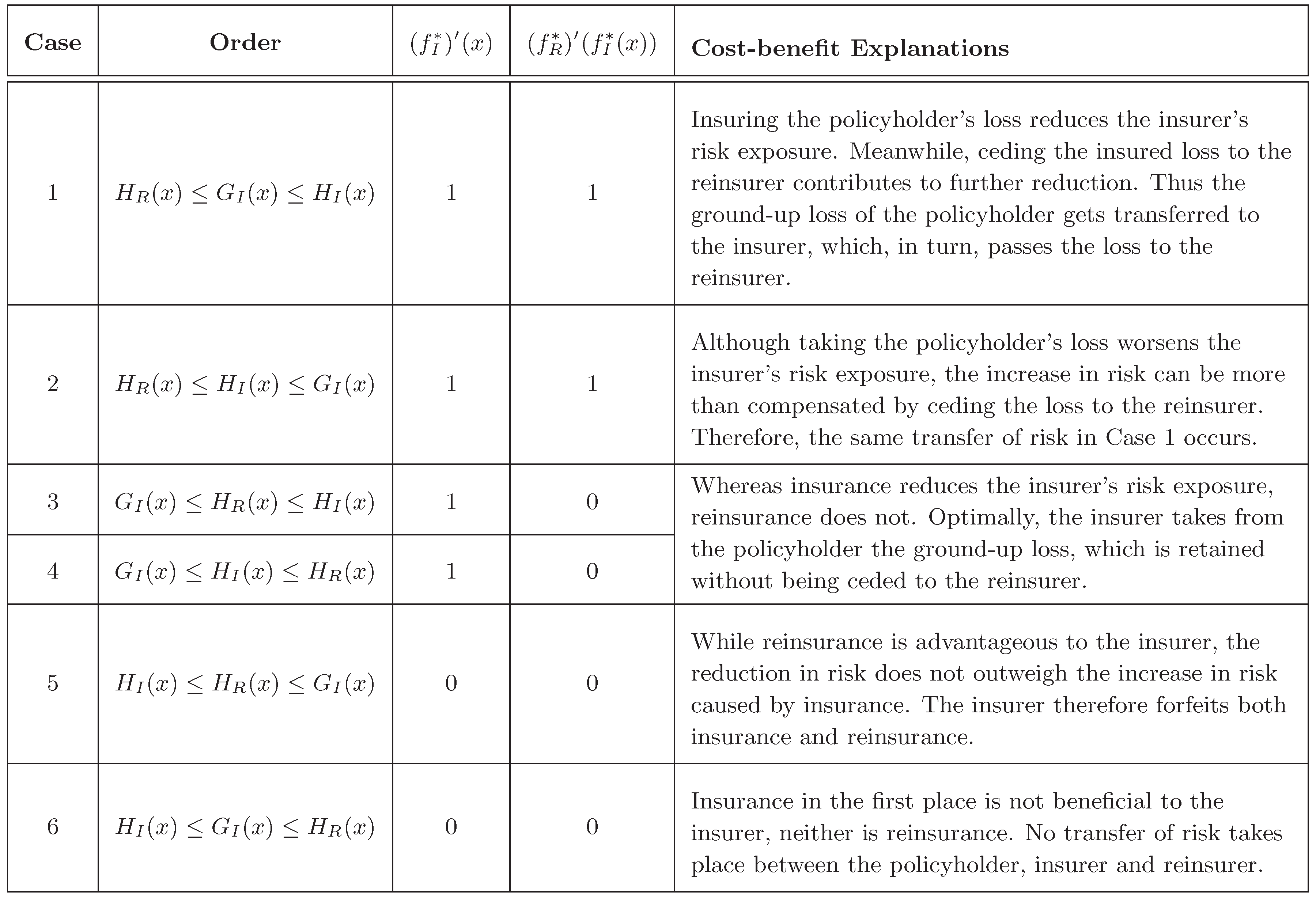
Armed with the cost-benefit identification above, we now list and explain all possible optimal insurance–reinsurance decisions in Figure 2 classified in accordance with the six different orders on the functions and . Note that, although some cases result in the same insurance–reinsurance policies, the motivations behind them can be different. Intuitively, the value that reinsurance creates manifests itself through two distinct channels:
- The losses that the insurer has decided to bear from the policyholder in the absence of reinsurance (which means , or ) may now be ceded to the reinsurer to contribute to further reduction in the insurer’s risk exposure, provided that the marginal benefit of reinsurance captured by the marginal increase in risk exposure, which is on and on ) outweighs the marginal cost of reinsurance represented by the marginal reinsurance premium . Mathematically, reinsuring the originally underwritten losses is profitable to the insurer if the cost-benefit difference of reinsurance defined in Formula (5) is non-positive. This is embodied by Case 1 in Figure 2.
- The access to reinsurance opens up new business opportunities to the insurer in that losses that are previously injudicious to assume from the policyholder (because ) may now be borne (because ) to the insurer’s advantage. While underwriting these losses from the policyholder undesirably increases the insurer’s risk exposure, transferring these losses to the reinsurer will generate a decrease that outweighs the preceding increase, leading to an overall drop in the insurer’s risk exposure. This corresponds to Case 2 in Figure 2.
The precise value that reinsurance brings with respect to the above two channels is mathematically formalized in the following corollary, which is a by-product of Theorem 1.
Corollary 1.
(Extra value introduced by reinsurance) The change in the insurer’s risk exposure before and after reinsurance is
In particular, in the absence of default risk (i.e., or ), the change in the insurer’s risk exposure is
Proof.
Before reinsurance, the optimal insurance contract is defined by Formula (16). The DRM of the insurer’s risk exposure is
When reinsurance becomes available, the optimal insurance and reinsurance contracts are given in Theorem 1. It follows from Equation (11) that the DRM of the insurer’s risk exposure after reinsurance is
The sum of the first and second integrals is
and the sum of the third and fourth integrals equals
Comparing the sum of Equations (18) and (19) to Equation (17), one observes that the change in the DRM of the risk exposure of the insurer is
☐
Compared to Proposition 3.2 of Zhuang et al. [11], Corollary 1 showcases more explicitly the structure of the value of reinsurance and attributes it to the two sources identified earlier, with
accounting for the additional decrease in the insurer’s risk exposure by ceding currently underwritten loses to the reinsurer, and with
explaining the contribution made by the new losses that the insurer finds it desirable to bear from the policyholder and cede to the reinsurer following the introduction of reinsurance.
3.3. Numerical Illustrations
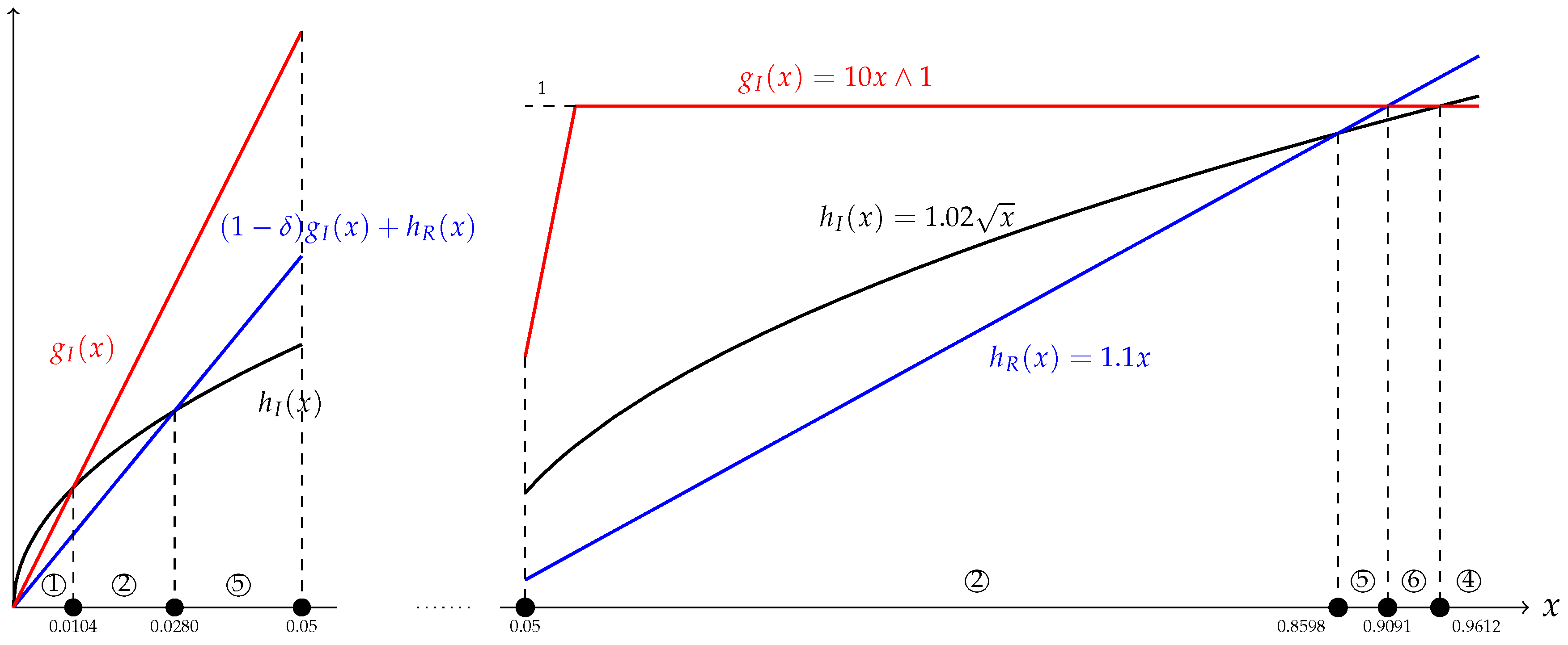
In this subsection, the analytic results and cost-benefit discussions in SubSection 3.1 and SubSection 3.2 are illustrated by a concrete numerical example with a view to examining the impact of reinsurance on the insurer’s optimal insurance decision. In particular, the possibility of Cases 1 and 2 in Figure 2 are demonstrated. Given the rising prominence of Tail Value-at-Risk (TVaR) in the banking and insurance industries (see, for example, BCBS [20]), we specifically assume that the insurer quantifies its risk exposure by means of the 90% TVaR, whose distortion function is given by
see Equation (45) of Dhaene et al. [17]. The insurance and reinsurance premiums are, respectively, calibrated by
i.e., the insurer and reinsurer, respectively, adopt the power distortion premium principle with a safety loading of and the expected value premium principle with a safety loading of . To reflect its prudence, the reinsurer sets its regulatory capital at the level of , and the recovery rate is . For concreteness, the ground-up loss X faced by the policyholder is taken as an exponential random variable with a mean of 1000 and p-level VaR given by .
The graphs of for and for are plotted in Figure 3. The comparison of the relative values of these functions will be instrumental in devising the optimal insurance and reinsurance contracts. Specifically, in the absence of reinsurance, the optimal insurance contract has full coverage on the losses where , leading to
which means that the insurer only bears small-sized and extraordinarily large-sized ground-up losses from the policyholder but leaves the medium-sized ones uninsured. When the insurer is endowed with reinsurance, the optimal insurance contract entails full coverage on the losses where for and where for . From Figure 3, we have
The corresponding reinsurance policy is given by
Comparing Formulas (20) and (21), one observes that the advent of reinsurance motivates the insurer to extend its coverage even to the losses between and and those between and , which are, in turn, ceded to the reinsurer. Doing so in the presence of reinsurance is advantageous to the insurer because the benefit stemming from the receipt of the insurance premium is able to offset the overall cost due to the payment of the reinsurance premium (or, in the case of extreme losses, the reinsurance premium coupled with the non-indemnified losses). Furthermore, the losses exceeding , which are insured under the original insurance policy, are also transferred to the reinsurer to gain a further reduction in the insurer’s risk exposure.
4. Conclusions
This article interweaves empirical findings and academic research on optimal reinsurance and studies the optimal insurance–reinsurance decisions made by an insurer in the context of a three-party model comprising a policyholder, insurer and reinsurer. Compared to existing research work in the literature, the novel contributions of this article are twofold. First, our analytic results have formed a stepping stone to understanding the cost-benefit implications of insurance and reinsurance for an insurer. The two channels through which reinsurance benefits an insurer are pinpointed and formalized. Second, it is shown both mathematically and intuitively that the presence of the reinsurer’s default risk diminishes the benefit of reinsurance to the insurer. Such a reduction in benefit needs to be taken into account when formulating the optimal insurance–reinsurance strategies.
The emphasis of this article is placed on how the interplay between insurance and reinsurance creates value to an insurer. Our one-period model, which may appear to be prototypical, is mathematically tractable, but sufficiently rich in structure to shed light on the economic ramifications of insurance and reinsurance. To avoid obscuring the economics of insurance and reinsurance, we have not added complications which may enhance the practicability of our model at the expense of a substantial raise in the degree of technicalities. Practicalities that can be incorporated into the model include risk transfer strategies (e.g., securitization) that the reinsurer can adopt and various constraints that accommodate the interests of different parties, such as constraints on the insurer’s budget on reinsurance, target profitability level, the reinsurer’s risk exposure, etc. For a unifying approach to tackling constraints that exploits the intrinsic Neyman–Pearson nature of optimal insurance–reinsurance problems, see Lo [21].
Acknowledgments
The author would like to thank the anonymous reviewers for their careful reading and insightful comments. Support from a start-up fund provided by the College of Liberal Arts and Sciences, The University of Iowa, is gratefully acknowledged.
Conflicts of Interest
The author declares no conflict of interest.
Abbreviations
The following abbreviations are used in this manuscript:
| DRM | Distortion risk measure |
| VaR | Value-at-Risk |
| TVaR | Tail Value-at-Risk |
References
- J.D. Cummins, G. Dionne, R. Gagné, and A. Nouira. “The Costs and Benefits of Reinsurance.” Working Paper. 2008. Available online: https://ssrn.com/abstract=1142954 (accessed on 12 December 2016).
- T. Holzheu, and R. Lechner. “The Global Reinsurance Market.” In Handbook of International Insurance, 2nd ed. Edited by J.D. Cummins and B. Venard. New York, NY, USA: Springer, 2007, pp. 877–902. [Google Scholar]
- C. Bernard. “Risk Sharing and Pricing in the Reinsurance Market.” In Handbook of Insurance, 2nd ed. Edited by G. Dionne. New York, NY, USA: Springer, 2013, pp. 603–626. [Google Scholar]
- J.E. Tiller, and D.F. Tiller. Life, Health & Annuity Reinsurance, 4th ed. Winsted, MN, USA: ACTEX Publications, 2015. [Google Scholar]
- K. Borch. “An attempt to determine the optimum amount of stop loss reinsurance.” Trans. Int. Congr. Actuar. 1 (1960): 597–610. [Google Scholar]
- K. Arrow. “Uncertainty and the welfare economics of medical care.” Am. Econ. Rev. 53 (1963): 941–973. [Google Scholar]
- J. Cai, K.S. Tan, C. Weng, and Y. Zhang. “Optimal reinsurance under VaR and CTE risk measures.” Insur. Math. Econ. 43 (2008): 185–196. [Google Scholar] [CrossRef]
- Y. Chi, and K.S. Tan. “Optimal reinsurance under VaR and CVaR risk measures: A simplified approach.” ASTIN Bull. 41 (2011): 487–509. [Google Scholar]
- W. Cui, J. Yang, and L. Wu. “Optimal reinsurance minimizing the distortion risk measure under general reinsurance premium principles.” Insur. Math. Econ. 53 (2013): 74–85. [Google Scholar] [CrossRef]
- A. Lo. “A unifying approach to risk-measure-based optimal reinsurance problems with practical constraints.” Scand. Actuar. J., 2016. [Google Scholar] [CrossRef]
- S.C. Zhuang, T.J. Boonen, K.S. Tan, and Z.Q. Xu. “Optimal insurance in the presence of reinsurance.” Scand. Actuar. J., 2016. [Google Scholar] [CrossRef]
- K.C. Cheung, and A. Lo. “Characterizations of optimal reinsurance treaties: A cost-benefit approach.” Scand. Actuar. J. 2017 (2017): 1–28. [Google Scholar] [CrossRef]
- A.V. Asimit, A.M. Badescu, and K.C. Cheung. “Optimal reinsurance in the presence of counterparty default risk.” Insur. Math. Econ. 53 (2013): 690–697. [Google Scholar] [CrossRef]
- J. Cai, C. Lemieux, and F. Liu. “Optimal reinsurance with regulatory initial capital and default risk.” Insur. Math. Econ. 57 (2014): 13–24. [Google Scholar] [CrossRef]
- D. Denneberg. Non-Additive Measure and Integral. Dordrecht, The Netherlands: Kluwer Academic Publishers, 1994. [Google Scholar]
- S. Wang. “Premium calculation by transforming the layer premium density.” ASTIN Bull. 26 (1996): 71–92. [Google Scholar] [CrossRef]
- J. Dhaene, S. Vanduffel, M.J. Goovaerts, R. Kaas, Q. Tang, and D. Vyncke. “Risk measures and comonotonicity: A review.” Stoch. Models 22 (2006): 573–606. [Google Scholar] [CrossRef]
- P. Jorion. Value at Risk: The New Benchmark for Managing Financial Risk, 3rd ed. New York, NY, USA: McGraw-Hill, 2007. [Google Scholar]
- S.C. Zhuang, C. Weng, K.S. Tan, and H. Assa. “Marginal Indemnification Function formulation for optimal reinsurance.” Insur. Math. Econ. 67 (2016): 65–76. [Google Scholar] [CrossRef]
- Basel Committee on Banking Supervision. Consultative Document October 2013. Fundamental Review of the Trading Book: A Revised Market Risk Framework. Basel, Switzerland: Basel Committee on Banking Supervision, Bank for International Settlements, 2013. [Google Scholar]
- A. Lo. “A Neyman-Pearson perspective on optimal reinsurance with constraints.” ASTIN Bull. forthcoming.
Figure 1.
The marginal costs and benefits of insurance (top) and reinsurance (middle and bottom) to the insurer.
Figure 1.
The marginal costs and benefits of insurance (top) and reinsurance (middle and bottom) to the insurer.
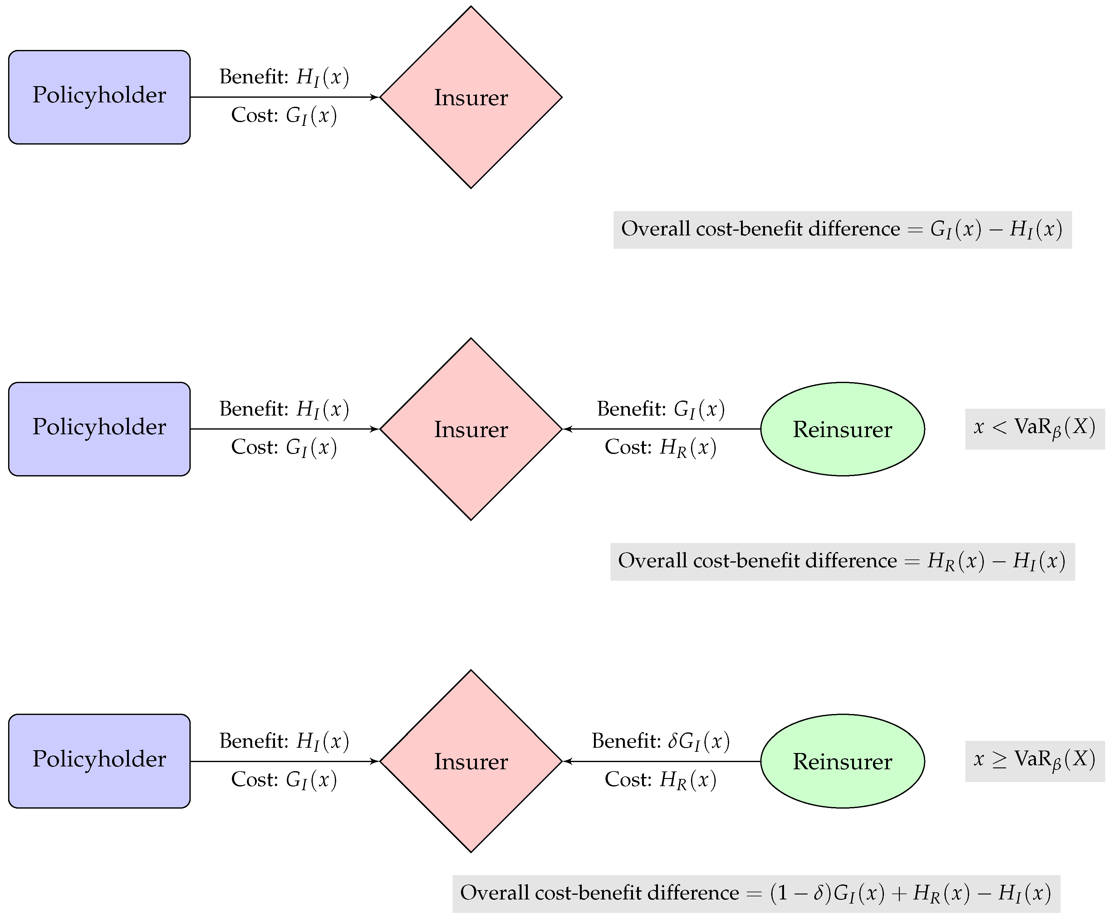
Figure 2.
Optimal insurance–reinsurance decisions corresponding to different orders of and when . The decisions for are obtained by replacing by in each case.
Figure 2.
Optimal insurance–reinsurance decisions corresponding to different orders of and when . The decisions for are obtained by replacing by in each case.

Figure 3.
The plots of for (left, magnified) and for (right). The circled numbers refer to the cases identified in Figure 2.
Figure 3.
The plots of for (left, magnified) and for (right). The circled numbers refer to the cases identified in Figure 2.
© 2016 by the author; licensee MDPI, Basel, Switzerland. This article is an open access article distributed under the terms and conditions of the Creative Commons Attribution (CC-BY) license (http://creativecommons.org/licenses/by/4.0/).
Share and Cite
MDPI and ACS Style
Lo, A. How Does Reinsurance Create Value to an Insurer? A Cost-Benefit Analysis Incorporating Default Risk. Risks 2016, 4, 48. https://doi.org/10.3390/risks4040048
AMA Style
Lo A. How Does Reinsurance Create Value to an Insurer? A Cost-Benefit Analysis Incorporating Default Risk. Risks. 2016; 4(4):48. https://doi.org/10.3390/risks4040048
Chicago/Turabian StyleLo, Ambrose. 2016. "How Does Reinsurance Create Value to an Insurer? A Cost-Benefit Analysis Incorporating Default Risk" Risks 4, no. 4: 48. https://doi.org/10.3390/risks4040048
Note that from the first issue of 2016, this journal uses article numbers instead of page numbers. See further details here.