
Dependence Uncertainty Bounds for the Expectile of a Portfolio


1
RiskLab, Department of Mathematics, ETH Zurich, 8092 Zürich, Switzerland
2
Faculty of Economics, Vrije Universiteit Brussel, Pleinlaan 2, 1050 Bruxelles, Belgium
*
Author to whom correspondence should be addressed.
Risks 2015, 3(4), 599-623; https://doi.org/10.3390/risks3040599
Submission received: 4 August 2015
/
Accepted: 4 December 2015
/
Published: 10 December 2015
Abstract
:We study upper and lower bounds on the expectile risk measure of risky portfolios when the joint distribution of the risky components is not fully specified. First, we summarize methods for obtaining bounds when only the marginal distributions of the components are known, but not their interdependence (unconstrained bounds). In particular, we provide the best-possible upper bound and the best-possible lower bound (under some conditions), as well as numerical procedures to compute them. We also derive simple analytic bounds that appear adequate in various situations of interest. Second, we study bounds when some information on interdependence is available (constrained bounds). When the variance of the portfolio is known, a simple-to-compute upper bound is provided, and we illustrate that it may significantly improve the unconstrained upper bound. We also show that the unconstrained lower bound cannot be readily improved using variance information. Next, we derive improved bounds when the bivariate distributions of each of the risky components and a risk factor are known. When the factor induces a positive dependence among the components, it is typically possible to improve the unconstrained lower bound. Finally, the unconstrained dependence uncertainty spreads of expected shortfall, value-at-risk and the expectile are compared.
1. Introduction and Preliminaries
This paper aims to contribute to the broader academic discussion on the properties of risk measures relevant to risk management and regulation in the banking and insurance industry; see [1] and [2] for an overview. The two most well-known risk measures are the value-at-risk (VaR) and expected shortfall (ES),
where the latter is only defined for random variables (rvs) X with a finite expectation. While VaR is dominantly used in industry, it lacks the property of subadditivity and is thus not coherent in the sense of [3]. By contrast, ES, which is merely the average of all upper VaRs, is coherent. In fact, it is the smallest coherent risk measure that is more conservative than VaR (see [3]). Recently, [4] brought the issue of elicitability to the foreground. A risk measure is said to be elicitable if it is a minimizer of the expectation of some scoring function, which depends on the point forecast and the true observed loss. The work in [4] showed that VaR is elicitable (if the corresponding quantile is unique), but ES is not. While some authors interpret this to mean that ES cannot be back-tested (e.g., [5,6]), [7] argue that elicitability is relevant for relative comparisons between estimators, but not for absolute significance testing. Moreover, [8] show that the pair (VaR, ES) is jointly elicitable. Nevertheless, the question arises whether there are non-trivial coherent risk measures that are elicitable. In [9,10,11], it is shown that the only risk measure that is both elicitable and coherent is the expectile. The expectile is introduced in [12] as the minimizer of the expectation of an asymmetric quadratic scoring function,
It follows that is the unique solution of the equation implied by the first order conditions (however, [13] points out that no differentiability or continuity of the distribution function is required):
Expectiles are well known in regression analysis [14,15,16]; they are used for forecasting financial time series [17] and estimating VaR and ES [18]. A penalized least squares approach in portfolio optimization was suggested by [19]; the expectile is a special case when a quadratic downside penalty is used. The expectile is also closely related to the Omega performance measure [20]; see [21], p. 128. The expectile was first explicitly considered as a risk measure in [22], and the authors coined the acronym EVaR. This name was later adopted in other articles ([23,24]). However, even the original authors admit that this acronym was already used for economic-VaR [25] and recently also for entropic-VaR [26]. To avoid confusion, we shall use the notation , as in [2,27] and [28], p. 290.
Throughout, we assume that the random variables represent losses. The expectile-based risk measure is subadditive and thus coherent for ; for this property, as well as other features and representations, see [13,27]. A discussion on risk management with expectiles can be found in [24]. In the present paper, we further contribute to this discussion by examining their properties when aggregating risks.
Note that by rearranging Equation (1),
Thus, the expectile can also be interpreted as the insurance premium using the Dutch premium principle (see [29]), where the insurer buys an excess-of-loss reinsurance contract for any claim above the premium e, with loading factor θ (and applies zero loading for the retained part). From Equation (2), we observe that expectiles are only implicitly defined, and their computation appears cumbersome. However, if the loss distribution is known, the following approach can be used to compute the corresponding expectile. First, define the tail integral,1 a function which will be useful for shorter notation,
Analytic expressions for are available for many commonly-used distributions, such as Pareto, log-normal, normal, Student t, exponential, gamma, and other. Next, applying Newton’s method to Equation (1) yields a practical iterative procedure for computing , given by:
where . An analogue for an empirical distribution using iterative reweighting is mentioned in [12] and stated explicitly in [14]. The convergence of this procedure is very fast. It is shown in [24] that for most common distributions, the expectiles are smaller than quantiles at level τ (for τ high enough), while for heavy-tailed (infinite variance) distributions, the opposite holds true. They coincide exactly (for all τ) for a Student t distribution with and asymptotically (as ) for the Pareto distribution. Therefore, initializing the procedure at appears reasonable.
While the expectile is a familiar object in regression analysis, its properties relevant to risk management are less studied. The focus of this paper is on risk aggregation and measurement under model uncertainty. Often the total (aggregate) loss that a company faces can be expressed as a sum , where the represent, e.g., the losses of different business lines or risk types. The risks are typically modeled separately, and little might be known about their interdependence. We will be interested in finding the range of values a risk measure can take for different aggregate losses , where is the so-called admissible class containing all of the aggregate loss distributions that are consistent with the available marginal and dependence information. In particular, define the best-possible upper bound and the best-possible lower bound as:
where the risk measure ρ will be either VaR, ES or the expectile. The idea to assess the impact of (partial) dependence information on risk bounds has been explored in a series of recent papers; see [30,31,32,33,34,35,36]. In these papers, the risk measure used was the VaR. In this paper, we will mainly focus on the expectile as a challenger for VaR.
The paper is structured as follows: Section 2 considers the case when only marginal distributions are known. We provide the best-possible upper bound, as well as the best-possible lower bound (under some conditions) and provide numerical procedures to practically compute these bounds. We also provide weaker bounds and show they are close to the best-possible ones in various situations of interest. We study the location-scale family and provide analytical expressions for the best possible bounds in this context. Section 3 gives bounds when the mean and variance of the aggregate loss are known. In Section 4, we consider the availability of dependence information through factor models. We provide various bounds in this context, and the results of this and previous sections are applied in an example using the skew-t distribution. In Section 5, the width of the dependence uncertainty interval for the expectile is compared to that of VaR and ES. Finally, Section 6 summarizes the observations.
2. Bounds when Only the Marginal Distributions Are Known
Due to the curse of dimensionality, it is typically easier to statistically fit a one-dimensional distribution function (df) to each than to fit a multivariate distribution to . Under an idealized version of dependence uncertainty (DU), only the marginal distributions , are known, while the dependence structure (copula) is completely unknown. Hence, the aggregate loss S can be any of the elements in the (Fréchet) admissible class ,
The (best-possible) bounds on the expectile are denoted by and . To determine the bounds, it turns out to be sufficient to find elements in that are maximal, respectively, minimal in the sense of convex order.2 We first recall the definition of this ordering concept and then connect it with and .
Definition 1 (Convex order) Let X and Y be random variables, such that:
provided the expectations exist. Then, X is said to be smaller than Y in the convex order ().
Consider the convex functions indexed by . We find that:3
In particular, this shows that upper bound , resp., lower bound , is obtained if one can find the maximum, resp., minimum element, in the convex order sense in the admissible class . The last implication in Equation (4) comes from the following lemma by taking and noting that . Specifically, the following lemma connects bounds on the stop-loss premium with bounds on .
Lemma 2. Suppose is a non-increasing function, such that:
Then, , where:
Analogously, a lower bound on the stop-loss premium yields a lower bound on .
Proof. From Equation (5), it immediately follows that:
Since for both inequalities, the right-hand side is non-increasing in e, the solution of Equation (2) (i.e., ) must be less than or equal to . ☐
2.1. Upper Bound with Marginal Information
It is shown in [40] that the comonotonic dependence structure leads to the maximal element (denoted ) with respect to the convex order in the admissible class .
Hence, we find that . In the case of identical margins , , using positive homogeneity, this simplifies to:
In general, however, the expectile is not comonotone additive, and hence, the upper bound often needs to be computed numerically. Unfortunately, the df of is typically not available in an analytical from, so the iterative procedure Equation (3) is more difficult to apply, since it would involve a nested root search. In particular, to compute at each step, one would first need to find a , such that , and then sum up the tail integrals for the margins.
Since is defined in Equation (7) in terms of its quantile function , it is easier to work in terms of the probability level p corresponding to the expectile. For continuous marginal distributions with densities , we can again apply Newton’s method by differentiating Equation (1) with respect to p using the chain rule. This yields an iterative procedure for computing in terms of , given by:
where and:
Again, since analytic expressions for the mean, the tail integral and inverse df of parametric marginal distributions are often available, this is a very fast and accurate method. It is possible that Equation (8) yields , in which case we can take instead; similarly, if , set . Analogously to Equation (3), it is reasonable to initiate the procedure at .
In general, by subadditivity (recall that we use ),
so is a valid upper bound, too, but it is typically not the best possible. In Section 4.3, is computed, as well as the best-possible upper bound in an example with skew-t distributions; we can observe that they are very close in all cases.
2.2. Lower Bound with Marginal Information
The analysis of the lower bound is more involved. We first observe that:
This can be seen either by applying Jensen’s inequality to the degenerate random variable to show , , or by noting that and that is increasing in τ (see, e.g., [24] for these and other properties). If the admissible class contains the constant , then this is the smallest element in convex order, and the lower bound Equation (10) is attained (sharp). This situation is achieved when the components are “compensating” for each other and corresponds to the notion of joint mixability, which was formally introduced in [41] and extends the concept of complete mixability ([42]) to the inhomogeneous case; see also [43] for an overview of these and related concepts. Precisely, a distribution F is called d-completely mixable if there exist rvs , , such that a.s., . Analogously, a d-tuple of dfs is called jointly mixable if there exist rvs , such that a.s., . Another concept that leads to an explicit smallest element in the Fréchet admissible class is that of mutual exclusivity, which requires that the margins have a large probability mass at an endpoint of the support; see [44].
In general, however, the dependence structure that leads to the smallest element in the convex order is known only for (countermonotonicity). If , for distributions that are bounded below (and satisfy some further conditions), in the case of identical margins, one can use the method from [45] (involves solving an integral equation), or for different margins, the method from [46] (requires solving a functional equation). A general, but approximate method is the rearrangement algorithm (RA) (see [47,48,49]), which is based on a discretization of the margins. In the following, we describe a simple, yet necessary modification of the RA that provides improved approximations for the best-possible lower bounds in the case of expectation-based risk measures, such as ES and the expectile.
2.2.1. Rearrangement Algorithm
The most general method currently available for computing lower bounds for the common risk measures is the RA; see [47,48,49]. While the quantile-based RA performs well when computing bounds on the (quantile-based) VaR, [50] indicates that for heavy-tailed margins, the RA lower bound for ES ([48]) is not sharp, because the tail expectation is underestimated due to discretization. Since also expectiles are defined in terms of the tail expectation (see Equation (2)), it is important to address this issue of the RA. In the following, we first recall the standard discretization of the RA for each margin and next provide two modifications that we further investigate.
| Standard RA: | , | . |
| Midpoint RA: | , | . |
| Expectation RA: | , | , |
| , |
While the standard discretization may seem conservative, it is nonetheless an approximate lower bound, since the RA may stop at a suboptimal rearrangement (see [48]). Moreover, if the distribution is unbounded below, then . For high N (such that ), this would still give a finite lower bound for ES; however, it would be undefined for the expectile, since it depends on both the upper and the lower tail of the aggregate distribution. The midpoint RA avoids this problem, but still underestimates tail expectations; the expectation RA should solve both issues. To evaluate and compare the sharpness of the bounds obtained using the different discretizations, we consider the homogeneous case with Pareto marginals. In this case, the exact lower bound on ES can be obtained using the method in [45]. In Table 1, the resulting underestimation errors are listed. Observe that the midpoint RA improves the results considerably, but the errors are still noticeable. The expectation RA, however, gives results that are within of the true lower bound. In light of this, we will use the “expectation” version of RA for computing the unconstrained lower bounds on the expectile (i.e., ) in Section 4.3, since it provides more accurate estimates of the tail expectations. One final adjustment concerns the stopping condition for RA. In [48], the RA stops when an iteration reduces the ES by less than a pre-defined ε. To match the stopping condition with the objective, we stop the RA when the reduction in becomes smaller than ε. This means that the expectile of the current rearrangement needs to be computed at each iteration. However, the Equation expectile of the previous iteration of the RA makes a very good initial guess for Equation (3), so this is not time-consuming. To summarize, the expectation RA only changes the way the margins are discretized and the stopping condition; the rest of the RA remains as in [48]. For other recent developments on the RA, we refer to https://sites.google.com/site/RearrangementAlgorithm/ and [51].

Table 1.
Relative underestimation as a percent of the exact for d Pareto distributions, using the rearrangement algorithm (RA) with different discretizations of size and stopping condition .
| Standard RA | ||||||||||||
| d | 1 | 2 | 3 | 4 | 5 | 8 | 1 | 2 | 3 | 4 | 5 | 8 |
| 0.1 | 0.2 | 0.2 | 0.2 | 0.3 | 0.4 | 0.3 | 0.5 | 0.6 | 0.7 | 0.8 | 1.2 | |
| 0.3 | 0.4 | 0.5 | 0.6 | 0.7 | 1.0 | 0.7 | 1.1 | 1.4 | 1.7 | 1.9 | 2.6 | |
| 0.5 | 0.7 | 0.9 | 1.0 | 1.2 | 1.5 | 1.2 | 1.7 | 2.2 | 2.6 | 2.9 | 3.8 | |
| 1.2 | 1.6 | 1.9 | 2.2 | 2.5 | 3.1 | 2.5 | 3.4 | 4.2 | 4.9 | 5.4 | 6.9 | |
| 5.3 | 6.6 | 7.6 | 8.3 | 9.0 | 10.6 | 9.0 | 11.5 | 13.4 | 14.9 | 16.2 | 19.4 | |
| Midpoint RA | ||||||||||||
| d | 1 | 2 | 3 | 4 | 5 | 8 | 1 | 2 | 3 | 4 | 5 | 8 |
| 0.0 | 0.0 | 0.0 | 0.0 | 0.1 | 0.1 | 0.1 | 0.1 | 0.1 | 0.1 | 0.2 | 0.2 | |
| 0.1 | 0.1 | 0.1 | 0.2 | 0.2 | 0.3 | 0.2 | 0.3 | 0.4 | 0.5 | 0.5 | 0.7 | |
| 0.2 | 0.2 | 0.3 | 0.3 | 0.4 | 0.5 | 0.4 | 0.6 | 0.7 | 0.8 | 1.0 | 1.3 | |
| 0.5 | 0.7 | 0.8 | 0.9 | 1.0 | 1.3 | 1.0 | 1.4 | 1.7 | 2.0 | 2.2 | 2.8 | |
| 3.0 | 3.8 | 4.3 | 4.7 | 5.1 | 6.0 | 5.1 | 6.5 | 7.5 | 8.3 | 9.0 | 10.6 | |
| Expectation RA | ||||||||||||
| d | 1 | 2 | 3 | 4 | 5 | 8 | 1 | 2 | 3 | 4 | 5 | 8 |
| 0.0 | 0.0 | 0.0 | 0.0 | 0.0 | 0.0 | 0.0 | 0.0 | 0.0 | 0.0 | 0.0 | 0.0 | |
| 0.0 | 0.0 | 0.0 | 0.0 | 0.0 | 0.0 | 0.0 | 0.0 | 0.0 | 0.0 | 0.0 | 0.0 | |
| 0.0 | 0.0 | 0.0 | 0.0 | 0.0 | 0.0 | 0.0 | 0.0 | 0.0 | 0.0 | 0.0 | 0.1 | |
| 0.0 | 0.0 | 0.0 | 0.0 | 0.0 | 0.0 | 0.0 | 0.0 | 0.1 | 0.1 | 0.1 | 0.1 | |
| 0.1 | 0.1 | 0.1 | 0.1 | 0.1 | 0.1 | 0.1 | 0.1 | 0.1 | 0.1 | 0.1 | 0.2 | |
2.3. Example: Location-Scale Family
We assume that the belong to the same location-scale family of dfs, i.e., , for some df F. Denote also and .
2.3.1. Upper Bound
By Equation (7), the convex order-maximal element in is given by:
Hence,
which can be computed using the procedure described in Equation (3). This also means that when the margins have the same shape, the bound based on subadditivity Equation (9) is the best possible.
2.3.2. Lower Bound
As mentioned before, obtaining an element in the admissible class that is minimum in the sense of convex order is often difficult or not even possible to achieve. However, in case the marginal dfs are from the same location-scale family that is symmetric, we can express the minimal element in the admissible class explicitly and, thus, also obtain the best-possible lower bound on the expectile.
Theorem 3. Let , belong to the location-scale family of a symmetric df F. Suppose without loss of generality that , .
- (i)
- If , then a minimal element in in convex order is:Correspondingly,
- (ii)
- Otherwise, if F furthermore admits a unimodal density, then the minimal element in the admissible class is the constant , and thus, .
Proof. (i) Case is trivial. If , we use the well-known fact that the convex order is consistent with the ordering of expected shortfall (note that ). In particular, Theorem 3.A.5 in [52] states that:
Clearly, and , have the required dfs, so . If F is continuous, then for any and any , we have that:
The first inequality follows from the fact that , and minimizes over events A of probability . Similarly, the second inequality follows because is maximal when .
If F is not continuous, then the indicators in Equation (11) need to be augmented by adding sets, such as:
to the first one (and similarly for the others). Since the dfs are symmetric and belong to a location-scale family, the atoms at , and , are of the same size.
In Case (ii), the rvs are jointly mixable by Corollary 3.6 in [41], and hence, the result follows. ☐
Note that Theorem 3 is of interest beyond the context of expectiles, as the convex order least element also yields lower bounds on, e.g., variance and ES in this admissible class. An early result in this direction was [53], where identical symmetric unimodal distributions with a differentiable density are considered. It is shown that for such a df F, there exist , , in the form , where and R is a continuous rv. Then, using that the uniform distribution is completely mixable (an explicit construction is given), it follows that also F is completely mixable. This model can be considered as a scale mixture of uniform distributions, where R is the scale factor, common to all margins. In Section 4, more general factor models are considered, and Theorem 3 is applied to find the minimal element in the convex order and to compute exact lower bounds in an example.
3. Bounds when the Mean and Variance of the Sum Are Known
We consider the case in which additional to the marginal information, also the variance of S is known, i.e., we consider the admissible class ,
where is a compatible variance constraint. In this setting, the bounds on will be denoted and . It is not so clear how to determine these best-possible bounds. Instead, we proceed by considering a larger admissible class that is easier to deal with,4 but gives weaker bounds. Note that in the case of VaR, in [30], it is shown that the weaker bounds are typically close to the best-possible ones. In the following sections, let , and denote:
3.1. Upper Bound with Variance Constraint
Since is a subset of , we find that where:
It will become apparent that variables supported on two points play an important role in the class .
Definition 4. A random variable is X called diatomic if and for some and .
The expectile of such a diatomic random variable has a simple expression,
Theorem 5. The maximum expectile B defined in Equation (13) is given by:
where . It is attained by a diatomic rv with support and mass τ at a, where:
Proof. Denote by the subset of diatomic variables. The proof further consists of two steps. First, we construct a variable that maximizes on . Next, we show that also provides the solution to Equation (13). Any has two support points with mass p at ,
where . Substituting and into Equation (14) yields:
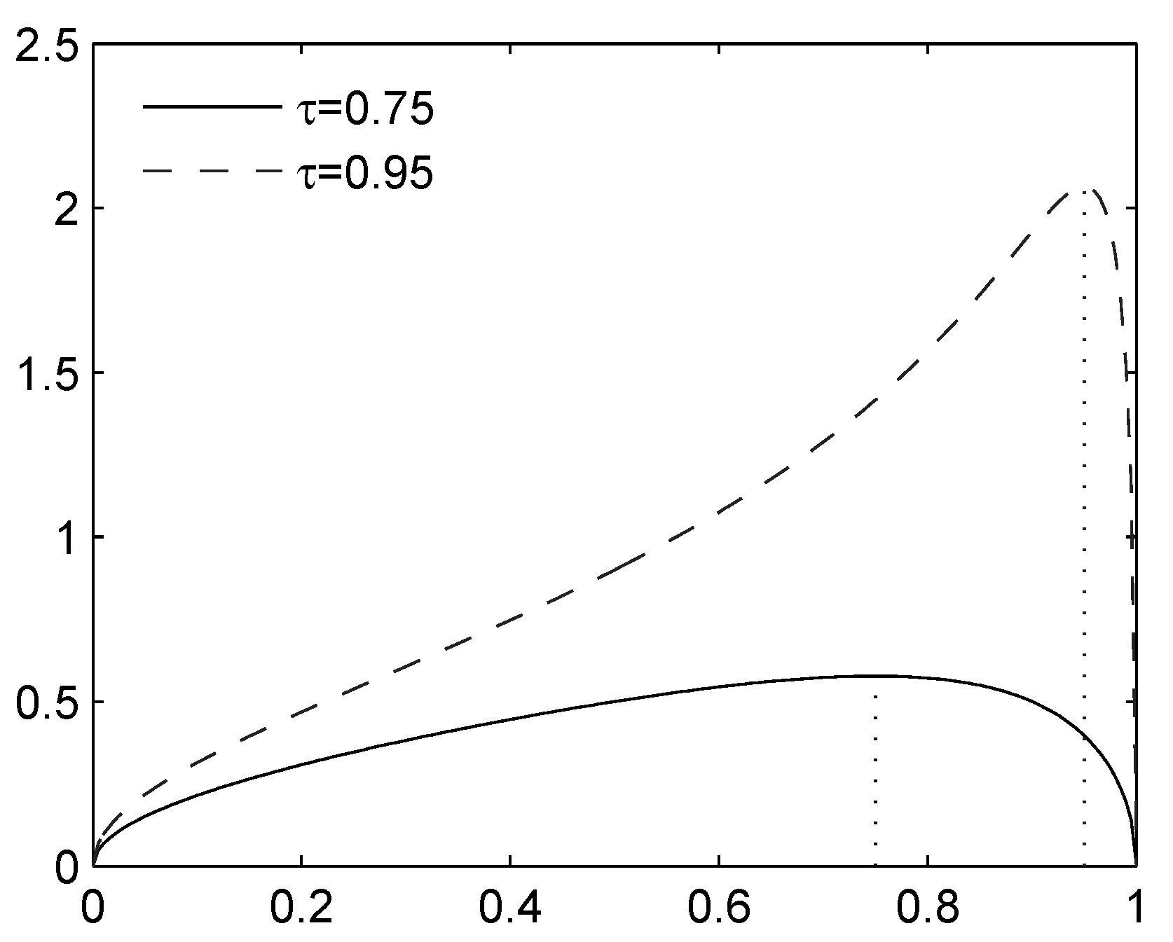
Figure 1.
Expectile for a diatomic rv (standardized to , ), as a function of . The maximum is attained at ; the minimum is approached as or .
Figure 1.
Expectile for a diatomic rv (standardized to , ), as a function of . The maximum is attained at ; the minimum is approached as or .

Using differentiation with respect to p, we find that attains its maximum on when (see also Figure 1). Hence, the variable that maximizes on is given by:
For this rv, defining , Equation (15) simplifies to:
Now, consider any . Without loss of generality, we can express for some standard uniformly distributed rv U. Letting , the variable S can also be written as:
Define a diatomic variable Y such that and by
From Jensen’s inequality, it follows that . Since Y is diatomic and the right-hand side of Equation (15) is increasing in s (recall that ),
which completes the proof. ☐
The bound B does not make use of the specific information on the marginal distributions. When the variance is “too high”, the unconstrained bound will be stronger. In the opposite case, B will dominate . We formulate the following corollary.
Corollary 6
Remarks.
- (i)
- A procedure called the extended rearrangement algorithm (ERA) was introduced in [30] and makes it possible to compute an approximation of from below, using both the marginal, as well as the variance information. This algorithm will be applied in an example in Section 4.3.
- (ii)
- Denote by and by . A similar proof as in Theorem 5 shows that C and D are attained by the same diatomic variable that attains the bound B; see also [30]. We find that:and, thus, that . On the other hand, the numerical value of these upper bounds would coincide for , and , if we set .
3.2. Lower Bound with Variance Constraint
From the proof of Theorem 5, it follows that:
is given by . Indeed, as , respectively ; see also Figure 1. Moreover, this bound cannot be improved by assuming either an upper bounded support or a lower bounded support.5 Hence, we conclude that working in the moment space does not make it readily possible to improve on .
4. Bounds for Factor Models
A factor model is introduced in [32] as a way to include additional information on the dependence structure and, hence, reduce the DU. This model considers rvs and a factor W for which the bivariate distributions of are known. The aggregate risk then belongs to the factor-constrained admissible class:
In the following, denote by the marginal distribution of and by the conditional distribution of , (if defined). The additional information of this factor structure leads to narrower factor-constrained DU bounds,
In the rest of this section, we consider a model where, conditional on a non-negative factor W with distribution G, the rvs belong to the location-scale family of distribution .
Models of this type are called location-scale mixture models and have a broad range of applications, going back to [55,56], where a particular location-scale mixture family (generalized hyperbolic) is introduced. In the area of financial modeling, [57] show that this family allows a good fit of asset returns; [58,59] apply it for pricing; and [60] apply it in the context of Garch models. Specific consideration has been given in the literature to sub-families of this class; see, for example, [61,62] for the case of the multivariate variance gamma distribution, as well as [63,64] for the case of multivariate skew-t distributions.
4.1. Upper Bound
According to Theorem 4.1 in [32], the largest element in the convex order is achieved in the case when, conditional on the factor, the margins are comonotonic. Thus, computing the upper bound on risk in such a model is as easy as computing , since the conditionally comonotonic sum belongs to the same class of location-scale mixtures:
and . In particular, we find that .
4.2. Lower Bound
The minimal element in the convex order sense is given by the following result (counterpart to Theorem 4.1 in [32]).
Theorem 7. If is a convex order-minimal element in for each w, then is a minimal element in and .
Proof. Since , it can be written as for some , . Thus, have the required bivariate distributions, and . To show it is minimal, consider any , and denote . By the definition of the convex order, for any convex function ϕ. Using monotonicity and the tower property, we obtain:
which completes the proof. ☐
Let . By Theorem 3, if the df in model Equation (16) is symmetric and unimodal, then a minimal element in is:
Thus, by Theorem 7, is a convex order minimal element in the factor-constrained admissible class. Moreover, since U is independent of W, also belongs to the same mixture family as the margins, so the corresponding lower bound can be computed as easily as . Note that the assumption that is symmetric is natural, since the location-mixing term can be used to add asymmetry to the df of .
4.3. Example: Skewed Student t Distribution
The results in Section 4.1 and Section 4.2 apply for general choices of dfs and G in Equation (16). The most well-known location-scale mixture class is that of normal mean-variance mixtures, i.e., the case when . If, in addition, W follows the generalized inverse Gaussian (GIG) distribution, then the family of generalized hyperbolic (GH) distributions is obtained; see Section 6.2.3 in [28]. This is a flexible class of distributions that exhibits skewness and heavy tails and is therefore useful for modeling financial data. Moreover, it can also be extended to the multivariate GH distribution,
where vectors in are written in bold, is the identity matrix and is the Cholesky decomposition of the scale matrix. The multivariate GH class is closed under linear operations, so it has the portfolio property, which is useful for applications. In this section, a particular subclass of GH is considered: the skew-t distributions.
The hyperbolic skewed Student t distribution is a special case of normal mean-variance mixtures, where the mixing distribution is the inverse-gamma df; see [64]. The inverse-gamma distribution has density:
Setting and in Equation (16) results in . The multivariate skew-t subclass of the GH distribution Equation (17) is also closed under linear transformations. Using Theorem 4.1 in [32], the factor-constrained worst-case dependence structure is achieved using A with as the first column and zeros in the others (conditional comonotonicity), resulting in a degenerate matrix Σ. The corresponding aggregate risk is:
Applying Theorems 3 and 7, the factor-constrained lower bounds in the “dominated” case (see Case (i) of Theorem 3) can be attained using A with σ as the first column, except in row i corresponding to the largest and zeros in other columns (conditional countermonotonicity with respect to the i-th margin). The corresponding aggregate risk is then:
The inverse df and tail integral (as well as the df and density) of a skew-t distribution can be computed using the methods in [65], which rely on the use of a Bessel function, numerical integration and root search (and are computationally intensive). Hence, we can apply the iterative algorithm Equation (3) (using the df and tail integral) to compute its expectile. Thus, we have a method to obtain the upper, respectively lower, factor-constrained DU bound. The unconstrained upper bound on the expectile can be computed using the iterative procedure Equation (8) (based on the tail integral, inverse df and density) and the unconstrained lower bound using the “expectation” version of RA introduced in Section 2.2.1.
Note that the conditionally jointly mixable case cannot be attained using a multivariate GH dependence structure. In this case, follows a scaled and translated inverse-gamma distribution. In order to apply the iterative procedure Equation (3), we need the df and tail integral (TI) for inverse-gamma. For a general , we calculate, using the substitution ,
which is the (normalized) incomplete gamma function. In MATLAB, this can be computed using the function gammainc(b./x,a,‘upper’). Similarly, we have:
which is given by b/(a-1)*gammainc(b./x,a-1,‘lower’) in MATLAB.
In Table 2, the expectile bounds for two examples of a skew-t distribution are listed. The parameters were selected to be in the range observed when fitting skew-t to daily stock returns (scaled by a factor of 250) of companies in the S&P100 index. Model A is a conditionally jointly-mixable case, and Model B is a “dominated” case. First, notice that the approximate upper bound is very close to the best-possible bound in all cases. Next, observe that due to the positive dependence the factor model induces, the value of the factor-constrained upper bound is similar to the unconstrained one, whereas the factor structure noticeably improves the lower bound; this is in agreement with the observations in [32]. In Model A, the unconstrained lower bound is close to the mean, so the margins are “almost” jointly mixable.
Table 2.
Upper and lower dependence uncertainty (DU) bounds for for two skew-t examples with . Column lists values for a multivariate skew-t distributed with a diagonal Σ matrix.
| Model A. | ||||||
|---|---|---|---|---|---|---|
| 0.8 | 1.24 | 2.16 | 13.70 | 35.58 | 35.62 | 35.63 |
| 0.9 | 1.24 | 3.02 | 21.63 | 57.14 | 57.21 | 57.22 |
| 0.95 | 1.24 | 4.14 | 29.65 | 78.73 | 78.85 | 78.87 |
| 0.99 | 1.25 | 8.44 | 51.18 | 135.63 | 135.98 | 136.02 |
| 0.999 | 1.30 | 23.30 | 96.78 | 251.11 | 252.65 | 252.84 |
| Model B. | ||||||
| τ | ||||||
| 0.8 | 1.91 | 2.18 | 19.34 | 34.58 | 34.61 | 34.62 |
| 0.9 | 2.50 | 3.01 | 30.68 | 55.29 | 55.36 | 55.37 |
| 0.95 | 3.15 | 3.99 | 41.90 | 75.74 | 75.84 | 75.86 |
| 0.99 | 5.15 | 7.34 | 70.80 | 128.00 | 128.28 | 128.31 |
| 0.999 | 10.05 | 17.51 | 126.92 | 228.06 | 229.15 | 229.29 |
In order to illustrate the influence of variance information on the bounds, we first need to find the feasible range for . The law of total variance yields:
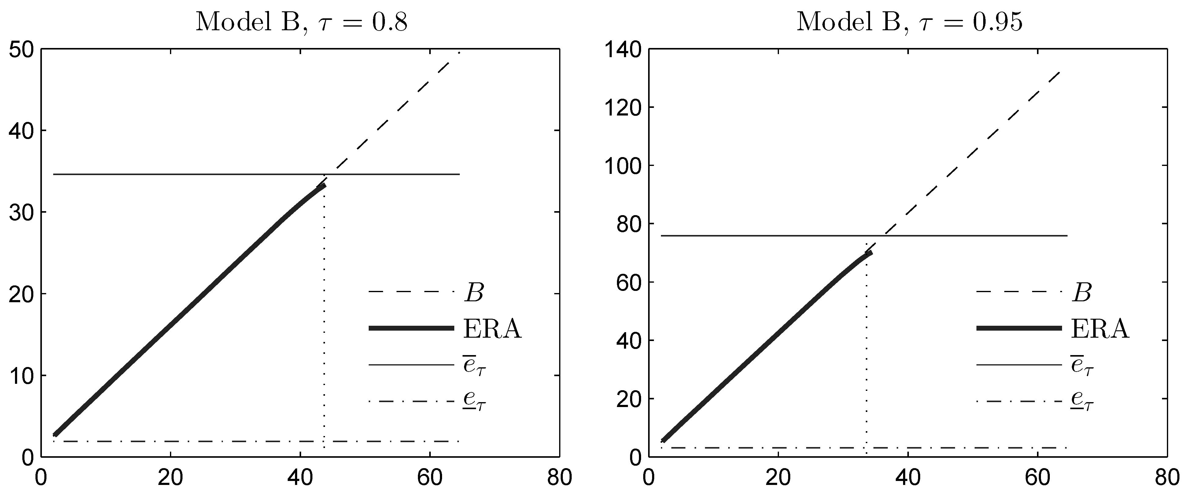
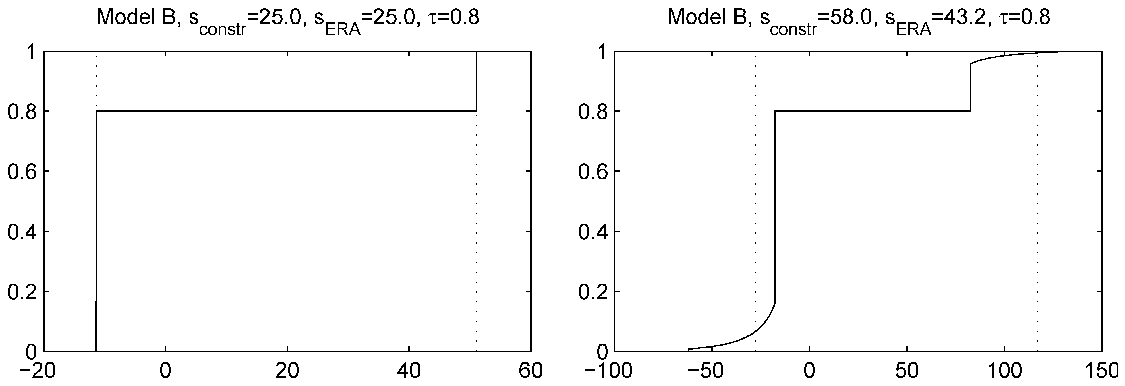
as long as . The first term lies in the range , corresponding to conditional joint mixability up to conditional comonotonicity. In Figure 2, we plot for Model B the variance-constrained bound B from Theorem 5 (based on the sole knowledge of the first two moments of the sum S), and we compare it with the unconstrained upper bound . We also plot the variance-constrained bound obtained by means of the extended rearrangement algorithm (ERA), which in addition to the first two moments of S, also takes into account the marginal distributions of the components (see [30] for a description of this algorithm). Variance constraints are taken in the range corresponding to standard deviation . We observe that variance information yields a considerably reduced upper bound B, as long as is small enough. As the parameter τ increases, the bound B becomes weaker and is relevant on a smaller range of . The approximate bound computed using ERA is very close to the bound B, indicating that B can nearly be attained by constructing the appropriate dependence among the random variables (with the given marginal distributions). This dependence yields a sum S that has a (nearly) diatomic structure, i.e., S becomes distributed as the random variable in Theorem 5. However, the highest variance that S can possibly attain, under the constraint that it is diatomic and consistent with the marginal distributions, occurs when its upper atom is given by . Therefore, when the variance constraint is too high, we cannot expect ERA to return a diatomic distribution for S; see also Figure 3, where the distribution function of S obtained using ERA is plotted for different variance constraints.
Figure 2.
Moment space upper bound B on the expectile, and an approximation of computed using the extended rearrangement algorithm (ERA), as a function of the standard deviation constraint s on the horizontal axis. The unconstrained expectile bounds are also plotted for the sake of comparison. The dotted vertical line is the maximum standard deviation of a diatomic random variable, which is consistent with the marginal upper- and lower-tail expectations.

Figure 3.
Distribution function of S computed using ERA for Model B, . In the left panel, a standard deviation constraint is applied and attained by ERA. In the right panel, a constraint is attempted, but cannot be attained, resulting in a lower actual standard deviation ; moreover, the distribution is not diatomic. The dotted lines are the optimal locations of the atoms from Theorem 5.
Remarks.
- (i)
- (ii)
- The most time-consuming quantity to compute was the unconstrained lower bound on the expectile, because the RA requires a discretization of the margins, i.e., calculating the skew-t inverse df times (each margin took about 10 min on an Intel i5 2.5 GHz desktop with ). A similar calculation with Pareto dfs as in Table 1 was done for this discretization size. The maximum error using the expectation RA was 0.4% for and 1.5% for ; hence, this discretization size was deemed sufficient for our purposes.
- (iii)
- Due to the mixture form of GH distributions, a faster method for discretizing the margins could be using a Monte Carlo sample. Since GH dfs can have heavy tails, a similar approach to the “expectation” discretization for RA was considered, specifically, rejecting any sample points that lie below or above and adding two points equal to the expectations over the corresponding intervals. However, this method resulted in a large variance over repeated trials, so the obtained bounds were not used.
4.4. Adding Variance Information
In this section, we consider factor models with additional variance information. We define the admissible class:
where the conditional variance is known for each outcome of W. Consider the problem:
Theorem 8. Let be given by:
where and . Then:
Proof. Let . By [54] (Case C), the upper bound6 on the stop-loss premium over (recall the definition of in Equation (12)) is given by:
which holds for any . Using monotonicity and the tower property, we obtain an upper bound for the unconditional stop-loss premium . Writing and invoking Lemma 2, we find that , where satisfies:
The stated equation for follows by rearranging. ☐
Remark. If the conditional variances are not known, but the total variance is available, then we still have that .
5. Dependence Uncertainty Spread Comparison
In this section, the dependence uncertainty (DU) spreads of VaR, ES and the expectile are compared, where the DU spread for a risk measure ρ is defined as:
Here, we focus on the Fréchet admissible class (only marginal dfs known); see Section 2. The behavior of DU spreads of VaR and ES for large-dimensional portfolios is discussed in [68]. In order to make the resulting capital requirements similar under the different risk measures, one could, for example, use the same level for all three, but multiply by different scaling factors.
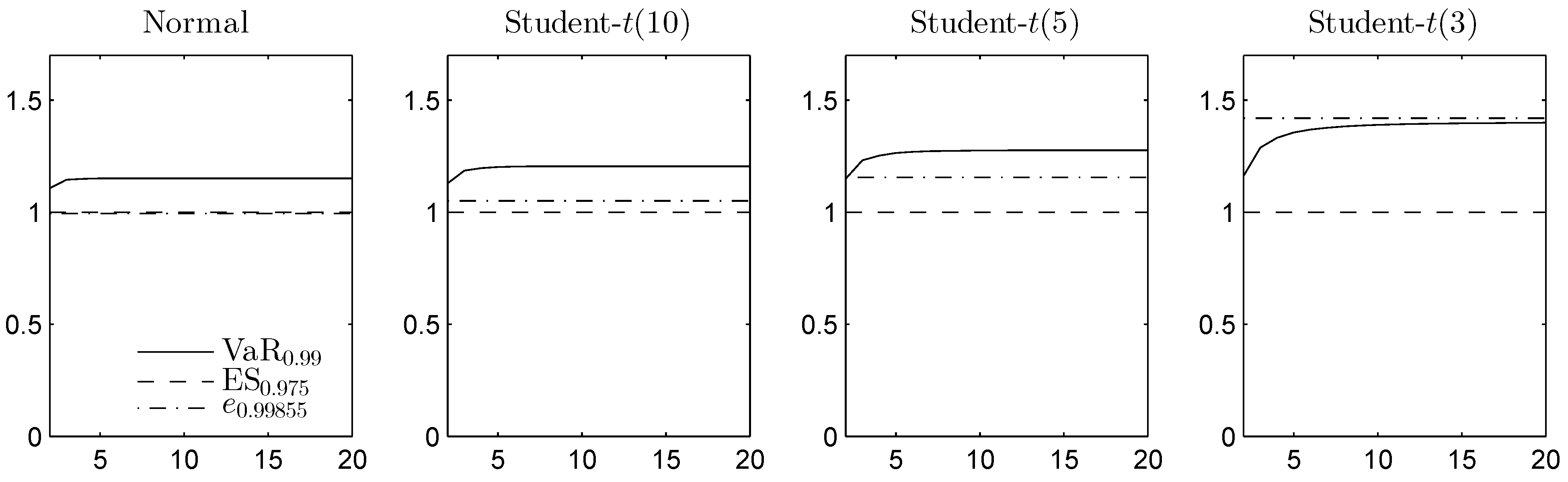
The approach taken by the Basel Committee on Banking Supervision [69], when moving from as the risk measure for the trading book capital requirements to ES, consists of adjusting the confidence level, apparently so that the numerical value of for a normally-distributed rv X matches . Doing so yields , which gets rounded to . Similarly, [24] suggest using a parameter τ, such that for ; this yields . Note that rounding to would give ; therefore, five significant digits will be used in this section when comparing the expectile to the other risk measures. ES is not as sensitive to the level β, and is close enough to .
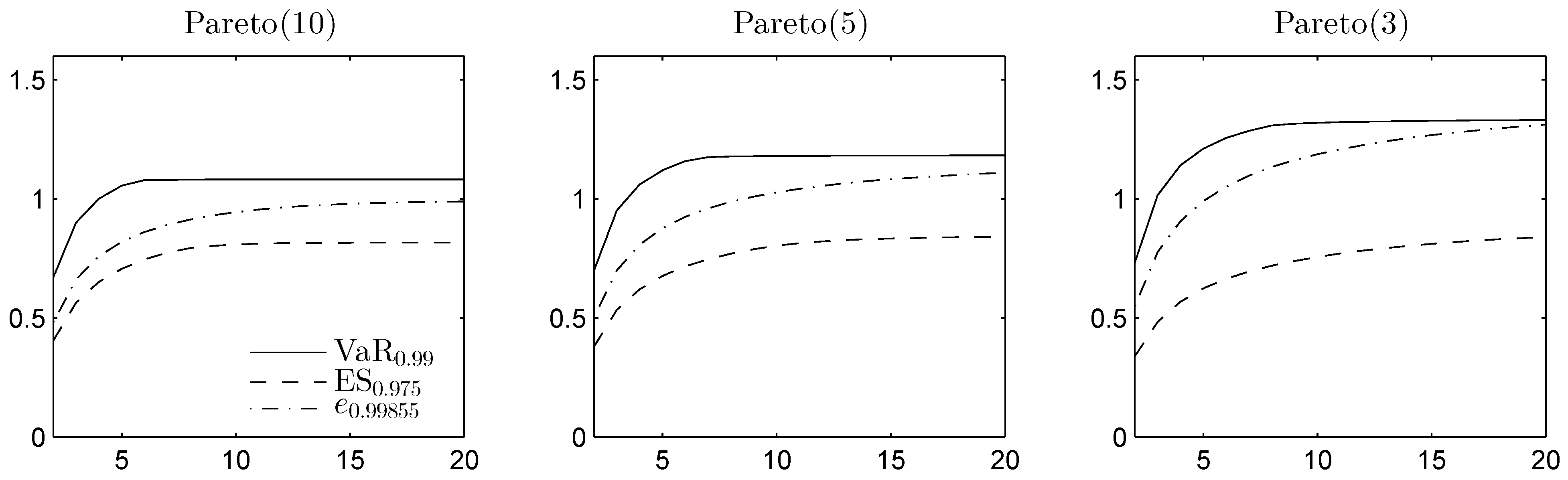
In Figure 4 and Figure 5, the DU spreads are plotted in the homogeneous case for different Pareto and Student t distributions, respectively, as functions of the dimension d. For the Pareto example, , , and are computed from the minimal elements in the convex order, obtained using the methods from [45]. and are obtained using the comonotonic dependence structure.
Since the Student t distribution is symmetric and unimodal, it is completely mixable [53], so the lower bounds on ES and the expectile are equal to the mean. To compute the lower bound on VaR, we apply RA. As the Student t density is decreasing from the median, [45] can again be applied for the upper bound on VaR. While VaR and ES focus only on the losses, the expectile also takes the gains into account. Student t has two infinite tails, which leads to a larger DU spread for the expectile, especially in the most heavy-tailed case. Overall, the results indicate that for the chosen adjusted significance levels, the DU spread is typically the smallest for ES.
Figure 4.
DU spread for VaR, expected shortfall (ES) and the expectile of the sum of d Pareto distributed margins, with d on the horizontal axis. The DU spread is given relative to .
Figure 4.
DU spread for VaR, expected shortfall (ES) and the expectile of the sum of d Pareto distributed margins, with d on the horizontal axis. The DU spread is given relative to .

Figure 5.
The DU spread for VaR, ES and the expectile of the sum of d Gaussian or Student distributed margins, with d on the horizontal axis. The DU spread is given relative to .
Figure 5.
The DU spread for VaR, ES and the expectile of the sum of d Gaussian or Student distributed margins, with d on the horizontal axis. The DU spread is given relative to .
6. Final Remarks
In the statistics literature, the expectile functional and its properties related to regressions are well known. Recently, in the context of risk measurement, the expectile risk measure has also been shown to have appealing theoretical properties. We contribute to the analysis of this new risk measure by focusing on its properties under dependence uncertainty. We first summarize and provide improved methods for computing bounds on the expectile of a portfolio in the case of no information on dependence (unconstrained bounds) and prove analytic bounds for a location-scale family. Next, we discuss the influence of dependence information on these unconstrained bounds.
In this regard, we provide simple-to-compute bounds under an additional constraint on the portfolio variance and show that the upper bound can be considerably improved. By contrast, the unconstrained lower bound cannot be improved by only using the information on the first two moments.
Furthermore, we provide bounds in the factor-constrained case. A family of commonly-used distributions, the normal mean-variance mixtures, is considered as a special case. These models are particularly tractable, and we state the conditional best- and worst-case dependence structures explicitly. We note that due to the restriction on dependence that such a factor model induces, the lower bounds were significantly improved (for high values of τ). The upper bounds are only slightly reduced, and the simple (unconstrained) upper bound based on subadditivity remains adequate for practical purposes.
We compare the dependence uncertainty spread of the expectile (i.e., the difference between the maximum and minimum possible value of the risk measure when only marginal information is used) with that of VaR and ES. We observe that the results are not favorable to the expectile. While the expectile has been proposed as the elicitable counterpart to ES, it is not clear that this property is indeed crucial for back-testing, and evidence exists to the contrary (e.g., [70]). Hence, gaining elicitability may not justify the increase in the dependence uncertainty spread. However, alternative mathematical approaches exist to “provide a broadly similar level of risk capture” ([71], p. 18) when moving to another risk measure (or even sticking with VaR), such as scaling. Although this makes the interpretation less clear (it was not clear for the expectile to begin with), it would allow reducing the confidence level, hence making statistical analysis more feasible and also reducing model uncertainty (see Table 2).
Acknowledgments
The authors thank Paul Embrechts and three anonymous referees for helpful comments and suggestions. E. Jakobsons thanks the Swiss Finance Institute for financial support. S. Vanduffel acknowledges the financial support from the Flemish Science Foundation (FWO).
Author Contributions
E.J. contributed mainly to the bounds with marginal information, examples and computations. S.V. contributed mainly to the bounds with variance information. The article was written in close collaboration.
Conflicts of Interest
The authors declare no conflict of interest.
References
- P. Embrechts, G. Puccetti, L. Rüschendorf, R. Wang, and A. Beleraj. “An academic response to Basel 3.5.” Risks 2 (2014): 25–48. [Google Scholar] [CrossRef] [Green Version]
- S. Emmer, M. Kratz, and D. Tasche. “What is the best risk measure in practice? A comparison of standard measures.” J. Risk 18 (2015): 31–60. [Google Scholar] [CrossRef]
- P. Artzner, F. Delbaen, J.M. Eber, and D. Heath. “Coherent measures of risk.” Math. Financ. 9 (1999): 203–228. [Google Scholar] [CrossRef]
- T. Gneiting. “Making and evaluating point forecasts.” J. Am. Stat. Assoc. 106 (2011): 746–762. [Google Scholar] [CrossRef]
- S. Kou, and X. Peng. “Expected shortfall or median shortfall.” J. Financ. Eng. 1 (2014): 1450007. [Google Scholar] [CrossRef]
- J.M. Chen. “Measuring Market Risk Under the Basel Accords: VaR, Stressed VaR, and Expected Shortfall.” Aestimatio IEB Int. J. Financ. 8 (2014): 184–201. [Google Scholar]
- C. Acerbi, and B. Szekely. “Back-testing expected shortfall.” Risk 27 (2014): 76–81. [Google Scholar]
- T. Fissler, and J.F. Ziegel. “Higher order elicitability and Osband’s principle.” Available online: arxiv.org/abs/1503.08123 (accessed on 30 September 2015).
- J.F. Ziegel. “Coherence and elicitability.” Math. Financ., 2014. [Google Scholar] [CrossRef]
- F. Bellini, and V. Bignozzi. “On elicitable risk measures.” Quant. Financ. 15 (2015): 725–733. [Google Scholar] [CrossRef]
- F. Delbaen, F. Bellini, V. Bignozzi, and J.F. Ziegel. “Risk measures with the CxLS property.” Financ. Stoch., 2015. [Google Scholar] [CrossRef]
- W.K. Newey, and J.L. Powell. “Asymmetric least squares estimation and testing.” Econom.: J. Econom. Soc. 55 (1987): 819–847. [Google Scholar] [CrossRef]
- F. Delbaen. “A remark on the structure of expectiles.” Available online: arxiv.org/abs/1307.5881 (accessed on 22 July 2013).
- B. Efron. “Regression percentiles using asymmetric squared error loss.” Stat. Sin. 1 (1991): 93–125. [Google Scholar]
- Q. Yao, and H. Tong. “Asymmetric least squares regression estimation: A nonparametric approach.” J. Nonparametr. Stat. 6 (1996): 273–292. [Google Scholar] [CrossRef]
- G. De Rossi, and A. Harvey. “Quantiles, expectiles and splines.” J. Econom. 152 (2009): 179–185. [Google Scholar] [CrossRef]
- C.W. Granger, and C.Y. Sin. “Modelling the absolute returns of different stock indices: exploring the forecastability of an alternative measure of risk.” J. Forecast. 19 (2000): 277–298. [Google Scholar] [CrossRef]
- J.W. Taylor. “Estimating value at risk and expected shortfall using expectiles.” J. Financ. Econom. 6 (2008): 231–252. [Google Scholar] [CrossRef]
- S. Manganelli. “Asset allocation by penalized least squares.” Available online: www.ecb.europa.eu/pub/pdf/scpwps/ecbwp723.pdf (accessed on 6 February 2007).
- C. Keating, and W.F. Shadwick. “A universal performance measure.” J. Perform. Meas. 6 (2002): 59–84. [Google Scholar]
- B. Rémillard. In Statistical Methods for Financial Engineering. Boca Raton, FL, USA: CRC Press, 2013. [Google Scholar]
- C.M. Kuan, J.H. Yeh, and Y.C. Hsu. “Assessing value at risk with CARE, the conditional autoregressive expectile models.” J. Econom. 150 (2009): 261–270. [Google Scholar] [CrossRef]
- G. De Rossi. “Staying ahead on downside risk.” In Optimizing Optimization: The Next Generation of Optimization Applications and Theory. Edited by S. Satchell. Waltham, MA, USA: Academic Press, 2009, pp. 143–160. [Google Scholar]
- F. Bellini, and E. di Bernardino. “Risk management with expectiles.” Eur. J. Financ., 2015. [Google Scholar] [CrossRef]
- Y. Aıt-Sahalia, and A.W. Lo. “Nonparametric risk management and implied risk aversion.” J. Econom. 94 (2000): 9–51. [Google Scholar] [CrossRef]
- A. Ahmadi-Javid. “Entropic value-at-risk: A new coherent risk measure.” J. Optim. Theory Appl. 155 (2012): 1105–1123. [Google Scholar] [CrossRef]
- F. Bellini, B. Klar, A. Müller, and E.R. Gianin. “Generalized quantiles as risk measures.” Insur.: Math. Econ. 54 (2014): 41–48. [Google Scholar] [CrossRef]
- A.J. McNeil, R. Frey, and P. Embrechts. Quantitative Risk Management: Concepts, Techniques and Tools, 2nd ed. Princeton, NJ, USA: Princeton University Press, 2015. [Google Scholar]
- A. Van Heerwaarden, and R. Kaas. “The Dutch premium principle.” Insur.: Math. Econ. 11 (1992): 129–133. [Google Scholar] [CrossRef]
- C. Bernard, L. Rüschendorf, and S. Vanduffel. “Value-at-Risk bounds with variance constraints.” J. Risk Insur., 2015. forthcoming. [Google Scholar] [CrossRef]
- V. Bignozzi, G. Puccetti, and L. Rüschendorf. “Reducing model risk via positive and negative dependence assumptions.” Insur.: Math. Econ. 61 (2015): 17–26. [Google Scholar] [CrossRef]
- C. Bernard, L. Rüschendorf, S. Vanduffel, and R. Wang. “Risk bounds for factor models.” Available online: papers.ssrn.com/sol3/papers.cfm?abstract_id=2572508 (accessed on 26 February 2015).
- G. Puccetti, L. Rüschendorf, D. Small, and S. Vanduffel. “Reduction of Value-at-Risk bounds via independence and variance information.” Scand. Actuar. J., 2015. forthcoming. [Google Scholar] [CrossRef]
- C. Bernard, and S. Vanduffel. “Quantile of a mixture with application to model risk assessment.” Depend. Model. 3 (2015): 172–181. [Google Scholar] [CrossRef]
- C. Bernard, L. Rüschendorf, S. Vanduffel, and J. Yao. “How robust is the value-at-risk of credit risk portfolios? ” Eur. J. Financ., 2015. [Google Scholar] [CrossRef]
- C. Bernard, and S. Vanduffel. “A new approach to assessing model risk in high dimensions.” J. Bank. Financ. 58 (2015): 166–178. [Google Scholar] [CrossRef]
- N. Bäuerle, and A. Müller. “Stochastic orders and risk measures: consistency and bounds.” Insur.: Math. Econ. 38 (2006): 132–148. [Google Scholar] [CrossRef]
- E. Jouini, W. Schachermayer, and N. Touzi. “Law invariant risk measures have the Fatou property.” In Advances in Mathematical Economics. Edited by S. Kusuoka and A. Yamazaki. Berlin, Germany: Springer, 2006, pp. 49–71. [Google Scholar]
- F. Bellini. “Isotonicity properties of generalized quantiles.” Stat. Probab. Lett. 82 (2012): 2017–2024. [Google Scholar] [CrossRef]
- A.H. Tchen. “Inequalities for distributions with given marginals.” Ann. Probab. 8 (1980): 814–827. [Google Scholar] [CrossRef]
- B. Wang, and R. Wang. “Joint mixability.” Math. Oper. Res., 2015. forthcoming. [Google Scholar] [CrossRef]
- B. Wang, and R. Wang. “The complete mixability and convex minimization problems with monotone marginal densities.” J. Multivar. Anal. 102 (2011): 1344–1360. [Google Scholar] [CrossRef]
- G. Puccetti, and R. Wang. “Extremal dependence concepts.” Stat. Sci., 2015. forthcoming. [Google Scholar]
- J. Dhaene, and M. Denuit. “The safest dependence structure among risks.” Insur.: Math. Econ. 25 (1999): 11–21. [Google Scholar] [CrossRef]
- C. Bernard, X. Jiang, and R. Wang. “Risk aggregation with dependence uncertainty.” Insur.: Math. Econ. 54 (2014): 93–108. [Google Scholar] [CrossRef]
- E. Jakobsons, X. Han, and R. Wang. “General convex order on risk aggregation.” Scand. Actuar. J., 2015. [Google Scholar] [CrossRef]
- P. Embrechts, G. Puccetti, and L. Rüschendorf. “Model uncertainty and VaR aggregation.” J. Bank. Financ. 37 (2013): 2750–2764. [Google Scholar] [CrossRef]
- G. Puccetti. “Sharp bounds on the expected shortfall for a sum of dependent random variables.” Stat. Probab. Lett. 83 (2013): 1227–1232. [Google Scholar] [CrossRef]
- G. Puccetti, and L. Rüschendorf. “Computation of sharp bounds on the expected value of a supermodular function of risks with given marginals.” Commun. Stat.—Simul. Comput. 44 (2015): 705–718. [Google Scholar] [CrossRef]
- P. Embrechts, and E. Jakobsons. “Dependence uncertainty for aggregate risk: Examples and simple bounds.” In The Fascination of Probability, Statistics and their Applications: In Honour of Ole E. Barndorff-Nielsen. Edited by M. Podolskij, R. Stelzer, S. Thorbjørnsen and A. Veraart. Berlin, Germany: Springer, 2016. [Google Scholar]
- M. Hofert, A. Memartoluie, D. Sunders, and T. Wirjanto. “Improved algorithms for computing worst Value-at-Risk: Numerical challenges and the Adaptive Rearrangement Algorithm.” Available online: arxiv.org/abs/1505.02281 (accessed on 9 May 2015).
- M. Shaked, and J.G. Shanthikumar. Stochastic Orders. Berlin, Germany: Springer, 2007. [Google Scholar]
- L. Rüschendorf, and L. Uckelmann. “Variance minimization and random variables with constant sum.” In Distributions with Given Marginals and Statistical Modelling. Berlin, Germany: Springer, 2002, pp. 211–222. [Google Scholar]
- F. De Vylder, and M.J. Goovaerts. “Analytical best upper bounds on stop-loss premiums.” Insur.: Math. Econ. 1 (1982): 163–175. [Google Scholar] [CrossRef]
- O.E. Barndorff-Nielsen. “Exponentially decreasing distributions for the logarithm of particle size.” In Proceedings of the Royal Society of London A: Mathematical, Physical and Engineering Sciences; 1977, Volume 353, pp. 401–419. [Google Scholar]
- O.E. Barndorff-Nielsen. “Hyperbolic distributions and distributions on hyperbolae.” Scand. J. Stat. 5 (1978): 151–157. [Google Scholar]
- O.E. Barndorff-Nielsen. “Normal inverse Gaussian distributions and stochastic volatility modeling.” Scand. J. Stat. 24 (1997): 1–13. [Google Scholar] [CrossRef]
- E. Eberlein, and U. Keller. “Hyperbolic distributions in finance.” Bernoulli 1 (1995): 281–299. [Google Scholar] [CrossRef]
- E. Eberlein, U. Keller, and K. Prause. “New insights into smile, mispricing, and value at risk: The hyperbolic model.” J. Bus. 71 (1998): 371–405. [Google Scholar] [CrossRef]
- K. Aas, I. Hobæk Haff, and X.K. Dimakos. “Risk estimation using the multivariate normal inverse Gaussian distribution.” J. Risk 8 (2005): 39–60. [Google Scholar]
- D.B. Madan, and E. Seneta. “The variance gamma (VG) model for share market returns.” J. Bus. 63 (1990): 511–524. [Google Scholar] [CrossRef]
- D.B. Madan, P.P. Carr, and E.C. Chang. “The variance gamma process and option pricing.” Eur. Financ. Rev. 2 (1998): 79–105. [Google Scholar] [CrossRef]
- S. Demarta, and A.J. McNeil. “The t copula and related copulas.” Int. Stat. Rev. 73 (2005): 111–129. [Google Scholar] [CrossRef]
- K. Aas, and I. Hobæk Haff. “The generalized hyperbolic skew Student’s t-distribution.” J. Financ. Econom. 4 (2006): 275–309. [Google Scholar] [CrossRef]
- S. Dokov, S.V. Stoyanov, and S. Rachev. “Computing VaR and AVaR of skewed-t distribution.” J. Appl. Funct. Anal. 3 (2008): 189–209. [Google Scholar]
- O.E. Barndorff-Nielsen, and C. Halgreen. “Infinite divisibility of the hyperbolic and generalized inverse Gaussian distributions.” Probab. Theory Relat. Fields 38 (1977): 309–311. [Google Scholar] [CrossRef]
- Y.S. Kim, S.T. Rachev, M.L. Bianchi, and F.J. Fabozzi. “Computing VaR and AVaR in infinitely divisible distributions.” Probab. Math. Stat. 30 (2010): 223–245. [Google Scholar] [CrossRef]
- P. Embrechts, B. Wang, and R. Wang. “Aggregation-robustness and model uncertainty of regulatory risk measures.” Financ. Stoch. 19 (2015): 763–790. [Google Scholar] [CrossRef]
- Basel Committee on Banking Supervision. Fundamental Review of the Trading Book. Basel, Switzerland: Bank of International Settlements, 2012. [Google Scholar]
- N. Costanzino, and M. Curran. “Backtesting general spectral risk measures with application to Expected Shortfall.” Available online: papers.ssrn.com/sol3/papers.cfm?abstract_id=2514403 (accessed on 21 February 2015).
- Basel Committee on Banking Supervision. Fundamental Review of the Trading Book: A Revised Market Risk Framework. Basel, Switzerland: Bank of International Settlements, 2013. [Google Scholar]
- 1.Note that for a continuous rv X, .
- 2.Likewise, the study of VaR bounds is connected to identifying (in an appropriate admissible class) the elements that are minimum in the sense of convex order, a feature that points to a similarity between the study of bounds on the expectile and the study of bounds on VaR; see Section 2.3 in [30] for these results.
- 3.Note that Equation (4) also follows from the more general results in [37,38]. Indeed, [37] has shown that any convex risk measure ρ with the Fatou property is consistent with the convex order, meaning that implies . Furthermore, [38] shows that law-invariant risk measures have the Fatou property. Since the expectile is convex and law invariant, it is consistent with the convex order. See [39] for further results on the properties of the expectile and other generalized quantiles with respect to various stochastic orders.
- 4.Note indeed that the admissible class reflects constraints rendering optimization difficult. By relaxing the d (infinite dimensional) constraints on the marginal distributions and substituting them by the portfolio mean constraint, we enlarge the class (as there are many marginal distributions that yield the same portfolio mean) and effectively obtain two constraints only, which greatly facilitates the optimization.
- 5.Assuming a compact support would improve the lower bound, but we do not elaborate on this case here and refer to [54].
- 6.This upper bound can also be derived using the reasoning in the proof of Theorem 5. Indeed, one shows that the upper bound is attained by a diatomic variable (with mean and variance ). Next, one optimizes over to obtain Equation (18).
© 2015 by the authors; licensee MDPI, Basel, Switzerland. This article is an open access article distributed under the terms and conditions of the Creative Commons Attribution license (http://creativecommons.org/licenses/by/4.0/).
Share and Cite
MDPI and ACS Style
Jakobsons, E.; Vanduffel, S. Dependence Uncertainty Bounds for the Expectile of a Portfolio. Risks 2015, 3, 599-623. https://doi.org/10.3390/risks3040599
AMA Style
Jakobsons E, Vanduffel S. Dependence Uncertainty Bounds for the Expectile of a Portfolio. Risks. 2015; 3(4):599-623. https://doi.org/10.3390/risks3040599
Chicago/Turabian StyleJakobsons, Edgars, and Steven Vanduffel. 2015. "Dependence Uncertainty Bounds for the Expectile of a Portfolio" Risks 3, no. 4: 599-623. https://doi.org/10.3390/risks3040599