
Multiparametric Guided-Mode Resonance Biosensor Monitoring Bulk and Surface-Film Variations

Department of Electrical Engineering, University of Texas at Arlington, Arlington, TX 76019, USA
*
Author to whom correspondence should be addressed.
Chemosensors 2022, 10(12), 541; https://doi.org/10.3390/chemosensors10120541
Submission received: 24 October 2022
/
Revised: 6 December 2022
/
Accepted: 12 December 2022
/
Published: 17 December 2022
(This article belongs to the Collection Optical Chemosensors and Biosensors)
Abstract
:A guided-mode resonance (GMR) sensor with multiple resonant modes is used to measure the collection of biomolecules on the sensor surface and the index of refraction of the sensor environment (bulk). The number of sensor variables that can be monitored (biolayer index of refraction, biolayer thickness, and bulk, or background, index of refraction) is determined by the number of supported resonant modes that are sensitive to changes in these variable values. The sensor we use has a grating and homogeneous layer, both of which are made of silicon nitride (Si3N4), on a quartz substrate. In this work, we simulate the sensor reflection response as a biolayer grows on the sensor surface at thicknesses from 0 to 20 nm and biolayer indices of refraction from 1.334 to 1.43 RIU; simultaneously, we vary the bulk index of refraction from 1.334 to 1.43 RIU. In the specified span of sensor variable values, the resonance wavelength shifts for 2023 permutations of the biolayer index of refraction, biolayer thickness, and bulk index of refraction are calculated and accurately inverted. Inversion is the process of taking resonant wavelength shifts, for resonant modes of a sensor, as input, and finding a quantitative variation of sensor variables as output. Analysis of the spectral data is performed programmatically with MATLAB. Using experimentally measured resonant wavelength shifts, changes in the values of biolayer index of refraction, biolayer thickness, and bulk index of refraction are determined. In a model experiment, we deposit Concanavalin A (Con A) on our sensor and subsequently deposit yeast, which preferentially bonds to Con A. A unique contribution of our work is that biolayer index and biolayer thickness are simultaneously determined.
1. Introduction
In industry, sensors/transducers have applications that include healthcare and medicine, air quality, food safety, and fuel storage. A problem in the aviation industry is the contamination of fuel with foreign organisms such as yeast [1,2,3]. The accumulation of bio-organisms, which feed on the carbon in fuels, reduces fuel stability, corrodes storage tanks, and degrades the functions of valves, pumps, and other mechanisms in a fuel system; all of these problems are termed fuel biofouling [4,5]. Portable transducers that are inexpensive, collect data for long time intervals, and generate data quickly after a binding event, can be used to monitor the status of jet fuel stored in tankers.
When detecting chemicals or organisms, it can be important to quantify the thickness and index of refraction of an adhered layer of analyte on the transducer surface, as well as the refractive index of the background/bulk media [6,7]. Quantifying these three variables requires multiparametric transducer input; in the case of a GMR sensor, these are three or more resonant peaks that shift due to these sensor variables [6]. A GMR sensor produces resonant peaks when interrogated with white light. As the sensor variables change, the wavelengths of the resonant peaks shift, and these shifts can be correlated to the magnitude that the sensor variables have changed [6,8].
Past work has determined sensor variable values using a sensor’s sensitivity, and the magnitudes of resonant wavelength shifts are monitored as one sensor variable is fixed and the other sensor variables are solved for [9]. This method usually requires that one biolayer variable is held constant as the other varies [10,11]. The sensitivities can be expressed as:
These expressions denote the biolayer index of refraction sensitivity {S(nbio)}, biolayer thickness sensitivity {S(dbio)}, and bulk index of refraction sensitivity {S(nbulk)}, respectively. In the above expressions, Δλ, Δnbio, Δdbio, and Δnbulk are the change in resonance wavelength, change in biolayer index of refraction, change in biolayer thickness, and change in bulk (background) index of refraction, respectively. Using sensitivity to determine biolayer sensor values falls short because the biolayer thickness (biolayer index of refraction) sensitivity is dependent on the value of the biolayer index of refraction (biolayer thickness). For instance, a greater biolayer thickness yields a greater absolute value of biolayer index of refraction sensitivity. This is because the evanescent tail of a resonant mode sees a larger change for a thicker layer. The analogue of this concept applies to the magnitude of biolayer thickness sensitivity: a greater biolayer index of refraction yields a greater absolute value of biolayer thickness sensitivity. Restricting one biolayer variable to a constant value, during biolayer growth, to calculate the other biolayer variable is a method to recon with the interdependence of the biolayer variables’ sensitivities; we avoid this restriction using our method of analysis. Our method expands on past work that used a GMR sensor with two resonant modes and simulation tools to create a lookup table [6]. In the work performed by Magnusson et al., the lookup table is used to solve for the biolayer index of refraction and the bulk index of refraction, while biolayer thickness is held constant [6].
There have been methods proposed to interpret transducer output and deconvolve the biolayer/adlayer thickness and biolayer/adlayer index of refraction [12,13,14]. These works include using a surface plasmon resonance sensor to conduct two experiments to obtain two data sets, then interpreting the data to determine the dielectric constant and thickness of a dielectric layer [15]. Another related work discusses the theory of using a combination GMR-SPR (guided mode resonance-surface plasmon resonance) sensor with three resonant modes; among the three resonant modes, the biolayer sensitivities differ by orders of magnitude and the bulk sensitivities also differ, to a lesser extent [16]. Using the values of sensitivity, matrix methods are proposed to calculate the biolayer thickness, biolayer index of refraction, and bulk index of refraction [16]. In addition to a sensor being multiparametric, such as those mentioned above, it is also of great importance that a sensor does not require the analyte to be tagged or altered for detection (label-free) [17].
A bio-selective layer can be applied to the sensor surface to capture the desired analyte and reject other substances in the environment [4,6,18,19]. Thus, a GMR sensor can be tailored to detect an analyte of choice without the use of labels, as in label-free sensing. Multiparametric and label-free sensing is in high demand in industry, and it can be performed using a GMR sensor [6,20].
Other label-free sensors include surface plasmon resonance sensors, integrated interferometers, MEMS-based sensors, nano-sensors (rods and particles), Bragg grating sensors, photonic crystal-based sensors, ring-resonator sensors, ellipsometry, and grating coupled sensors [6,21,22]. Sensor schemas that utilize labels include immunomagnetic separation, polymerase chain reaction, and standard immunoassay; these sensor types use luminescent, radioactive, absorptive, and fluorescent labels [6]. Sensors that utilize labels require the extra step of altering the analyte for detection. In contrast, the GMR sensor surface is altered to selectively capture and detect the analyte of interest.
Surface plasmon resonance (SPR) sensors, which are most like GMR sensors, utilize a resonance effect at the interface between a dielectric and metal [23,24]. When a TM polarized electromagnetic wave reaches a dielectric and metal interface at a specific angle of incidence, the electromagnetic wave becomes evanescent at the interface while interacting with the free electrons in the metal [25]. This phenomenon produces an absorption minimum in the spectrum that has high angular and spectral sensitivity [26]. The linewidth of SPR sensors is large, and only a TM mode produces an SPR response. In contrast, GMR sensors have a smaller linewidth, preferred over a large one, and the resonance effect can be produced using both the TE and TM modes; this allows the monitoring of the changes in a greater number of sensor variables with mixed polarization states.
The GMR sensor produces resonant modes by diffracting incident broadband light into leaky waveguide modes, allowing standing waves to form in the sensor at specific wavelengths (frequencies) as eigenmodes [27]. The GMR properties that admit these selected wavelengths into the sensor (coupled in), also allow these wavelengths out of the sensor (coupled out). Because standing waves have allowed multiple photons to constructively interfere, the efficiency of the light coupled out of the sensor is high [27]. The light coupled out at high efficiency is referred to as being resonant. These resonant wavelength spectra are narrow and sensitive to changes on the surface of the GMR structure, for example, chemical reactions or the presence of a biomaterial [7,19,27,28].
Magnusson and Wang proposed the use of the GMR effect for sensor applications due to the GMR filter’s tunable properties, based on the resonance structure parameters and refractive indices [27]. Tibuleac et al. and Wawro et al. introduced new GMR biosensor devices, in addition to applications of the sensors integrated with optical fibers [7,29]. Utilization of modal and polarization differentiation for multiparametric biosensors is a pivotal attribute of this technology [6].
GMR sensors are highly sensitive to their resonance parameters, which is innate in the fundamental resonance effect [6]. The resonant wavelength values of the GMR device are perturbed as the structure parameters change due to the attachment of a biomolecular layer on the device. A bio-selective layer on the GMR device can preferentially bind with a target analyte; this avoids additional data processing and foreign tags [6]. The GMR sensor has attributes including enriched data sets, label free sensing, and economic fabrication. These are qualities that will lead to the continued application of this sensor technology in several fields [30].
The sensor used in this work is required to have three or more resonant modes and it must be easily fabricated. To achieve the goal of three or more resonant modes, a sensor with a relatively thick homogeneous layer is developed. The thick homogeneous layer supports the resonant modes well. Here, we fabricate a 1-D grating with a two-part period. In addition, an aspect ratio is chosen so that the pillars in the grating are easily formed with a low probability of collapsing.
The sensor model shown in Figure 1a is simple and easily fabricated with a grating aspect ratio of 0.81. In Figure 1b,c the TM and TE spectra are shown for a simple grating (dh = 0 nm) and for dh values from 300 to 500 nm; these simulations use the rigorous coupled-wave analysis (RCWA) module in the RSoft DiffractMOD software (Synopsys, Inc., Mountain View, USA) [31,32]. The grating without a homogenous layer has no resonant peaks in the spectrum of interest. At a dh value of 500 nm, two resonances occur in each polarization state for a total of four resonant peaks. The thicker homogeneous layer results in more resonant peaks that are used to detect changes in the multiple sensor variables. To this end, a homogeneous layer of 500 nm is chosen for this work to allow for multiparametric data collection from the sensor (Figure 1b,c green line).
In this work we use simulation tools, with our multiparametric sensor, to generate an extensive library of biolayer thicknesses, biolayer indices of refraction, bulk indices of refraction, and the associated resonant wavelength shifts produced by our sensor. We use our library (also termed lookup table) and an inversion algorithm to take an input of the measured shifts of three resonant wavelengths (measured in one spectrometer reading), and then output the shifts in the value of three sensor variables (biolayer thickness, biolayer index of refraction, and bulk index of refraction). This method of determining biolayer and bulk sensor value shifts is novel, specifically because we simultaneously determine shifts in the values of two biolayer variables. To add to the usefulness of our method, we also determine the shifts in value of one bulk variable. The creation of a lookup table through a quick automated process and the utilization of an inversion algorithm expands what can be executed with multiparametric sensors/transducers.
2. Experiments and Methods
2.1. Fabricated Sensor Specifications
The guided-mode resonance (GMR) sensor consisted of a quartz substrate overlayed with silicon nitride (Si3N4) via plasma enhanced chemical vapor deposition (PECVD). The Si3N4 was deposited at a rate of 290 Angstrom/min. After Si3N4 was deposited on the substrate, it was patterned using laser interference lithography (LIL) and reactive ion etching (RIE) to achieve the fill factor and grating depth needed (Figure 2).
The sensor described above was used to quantify Concanavalin A (Con A) and Yarrowia yeasts that bind to the sensor surface. The sensor surface was functionalized with Con A because it attracts the glycoproteins found on the cell wall of the yeasts [4]. The reflection response of the sensor was measured with an Ocean Optics USB4000-VIS-NIR spectrum analyzer via an Ocean Optics bifurcated optical fiber. The layout of the sensor setup is illustrated in Figure 3.
2.2. Yeast Cell Preparation
The yeast cells used were in a suspension media including 20% glycerol. The yeast cells were of the fungal genus Yarrowia in the Ascomycota phylum family. There are 4 to 6 chromosomes in the yeast cells, and the genome encodes 6448 genes [4]. The Yarrowia species of yeast characteristically form biofilms [33]. The yeast cells were reduced from a concentration of to cells/mL by diluting them in phosphate buffer saline (PBS).
2.3. Sensor Surface Functionalization
The methanol used in this work was from Sigma-Aldrich (St. Louis, MO, USA); Concanavalin A (Con A) and glutaraldehyde were from Santa Cruz Biotechnology, Inc. (Dallas, TX, USA); and (3-Aminopropyl)triethoxysilane (APTES) was from Acros Organics (Carlsbad, CA, USA).
The sensor surface was functionalized in accordance with the work carried out by Abdallah et al. [4]. The molecules used on the sensor surface were meant to promote specific binding to the desired analyte (yeast cells) and simultaneously reduce non-specific binding. The silane in the APTES solution was used to capture the protein Con A. Con A has a high affinity to bind to the polysaccharides that are readily found on the cell wall of yeasts—the analyte of choice [34].
First, the sensor was placed in 3% (3-Aminopropyl)triethoxysilane (APTES) and 97% methanol for 30 min to salinize the surface. The sensor was then gently agitated for 60 s in a 60:40 mixture of methanol and deionized (DI) water; it was then dried in a vacuum furnace for 30 min at a temperature of 95 °C and a pressure of 15 mm Hg. A mixture consisting of 0.7% glutaraldehyde (GA) and 99.3% DI water was prepared and the sensor was submerged in the mixture for 60 min. Subsequently, the sensor was agitated in DI water for 60 s. The sensor was then incubated in 1 mg/mL of Con A in PBS for 120 min; for part of this time, the reflection spectrum was measured, and the resonant wavelength shifts at the end of the period were recorded as the total shifts. Then, the sensor was placed in a DI water bath and gently agitated for 60 s. A dilution of yeast cells in PBS with a concentration of 8.25 × 10⁵ cells/mL was used to soak the sensor surface for 120 min; the spectrum was measured for part of the incubation period. The wavelength shifts at the end of the recorded portion of this interval were recorded as the total shifts.
2.4. Inversion: Translating Resonant Shifts to Sensor Variables
A lookup table of simulated resonance shifts, and corresponding sensor variable value changes was used to invert resonant shift values to changes in the biolayer and bulk environment of the sensor. The RCWA module in RSoft DiffractMOD software (Synopsys, Inc., Mountain View, USA) was used for all simulations in this work [32]. A valuable feature of RSoft is the ability to set a value range of GMR structure parameters (like depth/thickness and index of refraction) and step sizes through the value range. For example, the grating depth range can be set from 50 nm to 250 nm and the step size can be chosen as 10 nm. This would result in producing 21 simulations that iterate through grating depth values from 50 nm to 250 nm (i.e., 50, 60, 70, … 250 nm) with all other GMR parameters held constant. Each simulation consists of reflectance over a wavelength spectrum, with the wavelength range and resolution selected by the user. The RSoft software can also perform iterative RCWA calculations over multiple sensor parameters based on ranges of values and step sizes through the ranges set by the user.
To produce the lookup table in this work, the sensor’s structural parameters (period, fill factor, grating depth, and homogeneous layer depth) and indices of refraction of materials were held constant, and a biolayer was modeled on the sensor surface. The term, sensor variables, is used to refer to the values of the modeled biolayer and a value of the bulk environment. Iterative simulations were set to cycle through values of biolayer thickness, biolayer index of refraction, and the bulk index of refraction; each simulation generates the reflectance spectrum for a set of sensor variable values.
In our work, the iteration settings were as follows: the biolayer thickness range was 2 nm to 20 nm and the step size was 3 nm (i.e., 2, 5, 8, … 20 nm), the biolayer index of refraction range was 1.334 RIU to 1.430 RIU and the step size was 0.006 RIU (i.e., 1.334, 1.340, 1.346, … 1.430 RIU), and the bulk index of refraction range was 1.334 RIU to 1.430 and the step size was 0.006 RIU (i.e., 1.334, 1.340, 1.346, … 1.430 RIU). This resulted in 7 values of biolayer thickness, 17 values of biolayer index of refraction, and 17 values of bulk index of refraction. A simulation was performed for every permutation of the biolayer and bulk sensor variable values set by the user; this resulted in a total of 2023 reflectance spectra produced via RSoft simulation. We developed a MATLAB program to quickly evaluate the peak wavelength values for each of the 4 resonant modes by finding the maximum reflectance value in a wavelength range corresponding to a given mode. For a single simulation, a set of 4 resonant wavelengths, biolayer thickness, biolayer index of refraction, and bulk index of refraction were grouped together and inserted into a digital file referred to as the lookup table; this was all performed within our MATLAB program. The lookup table consisted of all permutations of the sensor variables set by the user and the corresponding resonant wavelength values for the 4 resonant modes. Our use of the iterative ability of RSoft and the MATLAB code we developed were key to taking experimental resonance wavelength shifts as input and producing GMR biolayer thickness, biolayer index of refraction, and bulk index of refraction as output. For the results reported herein, out of the set of 4 available modes (see Figure 1), we used the 3 modes with the highest sensitivity.
The experimentally measured wavelength shifts were taken as input and compared to the wavelength shifts from the lookup table using the formula . Here, ΔλTi is the change in resonant wavelength (Δλ) from the lookup table (T) for the resonant mode (i). ΔλEi is the change in resonant wavelength (Δλ) from the experimental input (E) for the resonant mode (i). The set of resonant wavelength shifts from the lookup table for which S is minimized correlates to a set of sensor variables that were taken as the output.
Let us detail how Smin was calculated. We determined the difference between the lookup table resonance wavelength shift for resonant mode TM0 and the experimental resonance wavelength shift for resonant mode TM0; this value was then squared. This computation was also performed for the TM1 and TE1 modes. These 3 values (one for each mode used) were summed and then square rooted to get S. This calculation was performed for all 2023 lookup table entries.
Of the 2023 lookup table entries, the 10 with the lowest values of S were kept (S1 to S10) and all others were discarded. The 2nd lowest value of S (S2) was used to gauge the significance of the 8 S values that were greater (S3 to S10). Any S3 to S10 value that had a percent difference from S2 that was greater than ~30% was discarded. Statistical analysis of our data led us to using ~30% as the best cutoff point. As stated above, each S value corresponded to an entry in the lookup table. The biolayer thicknesses, biolayer indices of refraction, and the bulk indices of refraction corresponding to the remaining values of S were averaged and taken as the output biolayer thickness, biolayer index of refraction, and bulk index of refraction. Finally, to verify, these 3 physical values, inserted into the RCWA simulation software, generated the set of Δλ(simulation) that was approximately equal to the set of Δλ(experimental); this fact supports our use of this method.
3. Results and Discussion
3.1. Lookup Table
In this work, a GMR sensor was designed via simulation with the goal of having three or more resonant modes (Figure 1b,c); this was carried out to monitor changes in the single bulk variable and dual biolayer variables during the detection of an analyte. The values of resonant shifts for three of the modes of the GMR sensor were simulated for a range of bulk and biolayer variable changes. The resonant modes chosen for simulation were TM0, TM1, and TE1. These resonant modes were chosen because they had the highest sensitivity to changes of bulk and biolayer sensor variables. The sensitivities were determined by shifting one sensor variable at a time, by a marginal amount, while holding the other two sensor variables constant. To calculate the sensitivities, the sensor variable values were chosen to be near the median based on the value ranges specified in Section 2.4: bulk index of refraction (1.382 RIU), biolayer thickness (11 nm), and biolayer index of refraction (1.388 RIU). For clarity, to determine the biolayer/adlayer index of refraction sensitivity, the value of bulk index of refraction was held constant at 1.382 RIU and the value of biolayer thickness was held constant at 11 nm, while the biolayer index of refraction was varied marginally; the ratio of resonance wavelength shift and biolayer index shift is the sensitivity. An analogous process was applied to determine the GMR sensor sensitivity to biolayer thickness shifts and bulk index of refraction shifts.
The bulk index of refraction sensitivity for each mode was calculated as: TM1 (56 nm/RIU), TM0 (21 nm/RIU), TE1 (65 nm/RIU), and TE0 (17 nm/RIU). The biolayer thickness sensitivity for each mode was calculated as: TM1 (0.0057 nm/nm), TM0 (0.0027 nm/nm), TE1 (0.0027 nm/nm), and TE0 (0.0013 nm/nm). The biolayer index of refraction sensitivity for each mode was calculated as: TM1 (12 nm/RIU), TM0 (5.8 nm/RIU), TE1 (4 nm/RIU), and TE0 (2.2 nm/RIU). All sensitivities were determined via simulation with rigorous coupled-wave analysis as referenced above. The bulk index sensitivities were approximately linear for the range considered in this study as supported by Figure 4.
Recapitulating, the purpose of our work and the sensor proposed is to have three resonant modes to enable multiparametric data collection for use with a lookup table and inversion algorithm.
Figure 5 is a visual representation of a small portion of the lookup table that is generated via simulation. Each data point represents a combination of biolayer index of refraction, biolayer thickness, bulk index of refraction, and the resultant resonance wavelength shift. The greater the slope of a line taken across a plane in Figure 5, the more sensitive the resonant mode is to changes in the biolayer. In addition, the greater the difference in resonance wavelength shift between the planes, in a plot for a given mode, the more sensitive the mode is to a change in the bulk index of refraction. While the TM1 and the TE1 modes of light have comparable sensitivities to the bulk index of refraction, the warped nature of the TM1 planes is indicative of the greater sensitivity to changes in the biolayer for the TM1 mode. The lookup table, which is visually represented in Figure 5, is used to invert from experimentally measured resonant wavelength shifts to changes in sensor variables.
The use of a lookup table of sets of resonance wavelengths with their accompanying sensor variable values is a novel aspect of our work. Specifically, the use of a lookup table to determine both biolayer thickness and the biolayer index of refraction in one spectral measurement is nuanced. Many past studies, focused on determining sensor biolayer variable values, are restricted to holding one biolayer variable constant as the other biolayer variable is solved for. Our method of analysis, using a lookup table, overcomes this issue. Additionally, we use our method to determine the bulk index of refraction. This enhances the use of sensors with multiparametric output. Equation (4) is the fully expanded equation used to determine the sensor variable values as applied in practice. Minimization of the differences between experimental and theoretical resonance shifts determines the sought sensor variables. Thus, we minimize:
The three resonant wavelength shifts are used to determine Smin, and Smin is used to determine the biolayer index, biolayer thickness, and bulk index. These four sets of values (Smin and the sensor variables) define the four-dimensional numerical space in which the inversion algorithm operates.
3.2. Simulated Input Wavelengths Compared to the Calculated Output Sensor Variable Values
The lookup table used in the inversion algorithm consists of 2023 simulations with three sensor variables, the values of which are specified in Section 2.4; each one of the simulations is used to generate a corresponding set of three resonant wavelength shifts. To test the accuracy of our method, a set of the three resonant wavelength shifts are used as input in the inversion algorithm to determine if the expected biolayer thickness, biolayer index of refraction, and bulk index of refraction are produced as the output. This test resulted in an accurate output for all 2023 permutations of biolayer and bulk value shifts. To further test the accuracy of the inversion algorithm, sensor variable sets with changes in biolayer thickness and biolayer index that deviate from those used to create the lookup table are chosen, and via simulation the corresponding resonance wavelength shifts for the TM0, TM1, and TE1 modes are determined. These sets of three resonance shifts are input into the inversion algorithm, and the output of the inversion algorithm is compared to the known shifts of sensor variable values (Table 1). In Table 1, Δnbio, Δdbio, and Δnbulk refer to the change in biolayer/adlayer index of refraction, change in biolayer/adlayer thickness, and change in bulk/background index of refraction, respectively.
The first three columns are the shifts in sensor variable values used in the RSoft RCWA simulations to generate resonant wavelength shifts. The resonant wavelength shifts are then used as input for the inversion algorithm. The last three columns are the algorithm output, namely, calculated shifts in sensor variable values. The change in bulk refractive index is calculated with very high accuracy because the values simulated exist in the lookup table and because a slight shift in bulk RIU results in significant resonant wavelength shifts. The calculated changes in biolayer refractive index and biolayer thickness have slight deviations from the input values. This is because the input values do not exist in the lookup table, so a direct match is not possible. However, the output of the algorithm is very close to the expected sensor variable shifts as seen by comparing the left three columns with the corresponding columns on the right.
In Table 1, the largest biolayer thickness deviation (that is the difference between the expected value and the value produced by the inversion algorithm) is 1.5 nm, the largest biolayer index of refraction deviation is 0.004 RIU, and the largest bulk index of refraction deviation is approximately 0 RIU. These relatively small deviations, and the accuracy of the inversion algorithm when values from the lookup table are used as input (this is described in detail at the beginning of this section), provide a strong case for the usefulness and credibility of our inversion algorithm.
3.3. Measured Resonance Shifts and Inversion for Con A Incubation
The experimentally measured reflection response of the fabricated sensor is shown in Figure 6, where four resonant peaks, within the wavelength spectrum of interest, are produced. In addition, Figure 6 shows that each peak position is distinguishable from other peaks, so a polarizer is not necessary to monitor the shifts in peak position. It is shown here that the wavelength shifts over time can be used to simultaneously monitor the growth of a biofilm on a sensor surface, as well as changes in the bulk index of refraction.
During the functionalization process, to prepare the sensor to receive the analyte, glutaraldehyde (GA) is used to activate the amine groups from the APTES already deposited on the sensor. During incubation in the solution of Con A and PBS, an amide bond is formed between Con A and the amine groups on the sensor surface; this immobilizes Con A on the sensor. After incubation in Con A, the sensor is washed in DI water. The measured resonant shifts for Con A detection are 0.074, 0.18, and 0.058 nm for TM0, TM1, and TE1, respectively. Table 2 shows the output sensor variables determined using the inversion algorithm.
Table 2 shows that the largest wavelength shift occurs for the TM1 mode, with smaller shifts for the TM0 and TE1 modes. This is in line with the TM1 mode being more sensitive to biolayer variable changes than the TM0 and TE1 modes. Additionally, the TM0 mode is more sensitive to biolayer thickness changes than the TE1 mode, and this accounts for TM0 having a greater resonant wavelength shift than TE1. The expectation is that Con A precipitates out of solution and adheres to the sensor surface due to the amide bond formed between Con A and the glutaraldehyde (GA) on the sensor surface. As Con A accumulates on the sensor surface during the incubation period, the shifts in the TM1 and TM0 modes are indicative of a change in the biolayer; because no process occurs that changes the bulk refractive index, the TE1 mode has a relatively small shift.
During Con A incubation, the reflection spectrum of the GMR sensor is recorded every ~10 s. We have included the spectrum of the measurements at 0.17 min and 80 min in Figure 7.
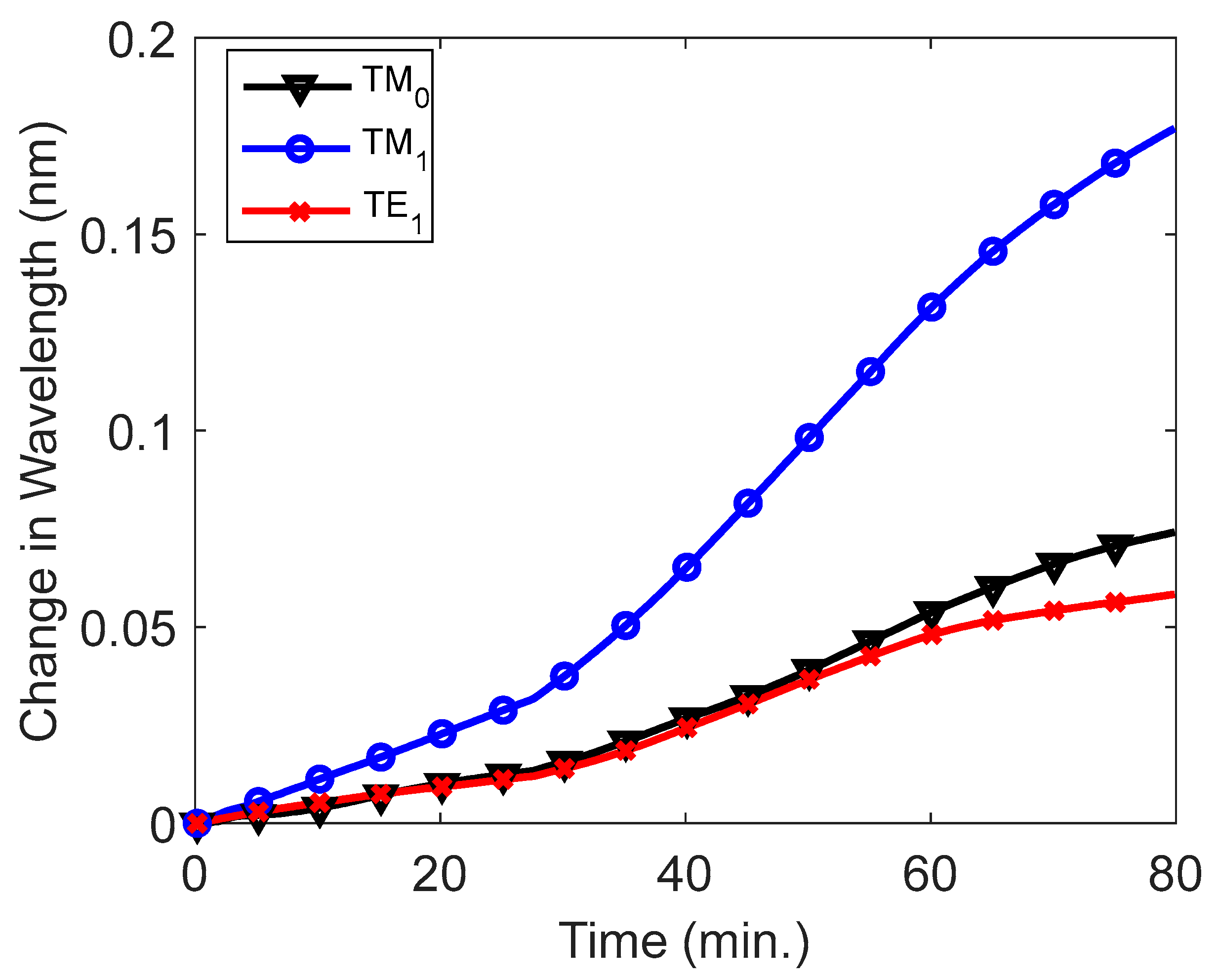
Figure 8 shows the increase in the resonant shifts for the three modes of interest over time: during incubation in the Con A and PBS solution. This increase in resonant wavelength shift over time is due to the gradual accumulation of Con A on the surface of the GMR sensor. The spot of the sensor being monitored was altered at the 80-min mark. Thus, monitoring the development of a biolayer in a single spot on the sensor was stopped and data collection ceased after 80 min. Using the measured shifts of the resonant modes in Figure 8, the sensor variables are calculated. The algorithm output shows the progressive accumulation of Con A on the sensor surface (Figure 9).
The biolayer index of refraction increases gradually until the ~70-min mark. After ~70 min the biolayer index of refraction stabilizes, and the shift is within the 0.006 RIU resolution of the lookup table. The biolayer thickness increases until the ~50-min mark. Thereafter, the biolayer thickness stabilizes, and the shift is within the 3 nm resolution of the lookup table.
3.4. Measured Resonance Shifts and Inversion for Yeast Incubation
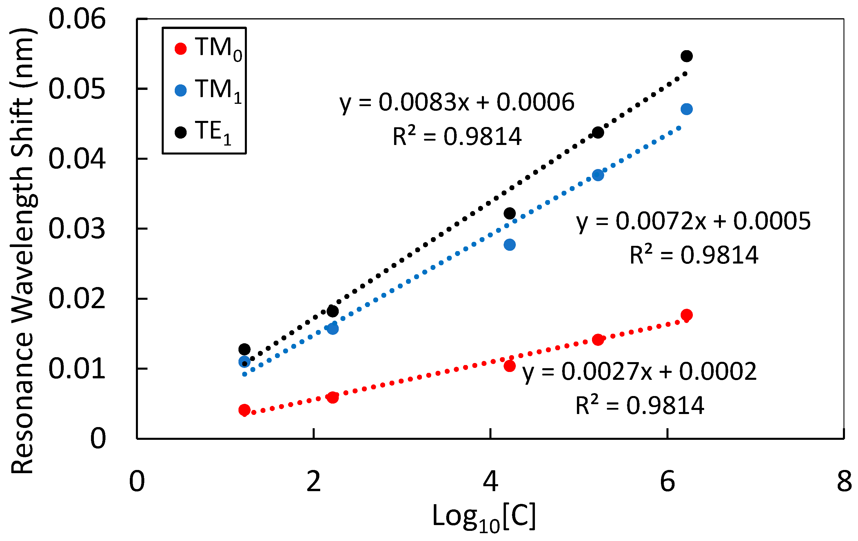
In our previous work with yeast cell detection, we calculated the limit of detection (LOD) to indicate the capability of the sensor used in that work [4]. Scaling the data collected in that work, by comparing the bulk sensitivity of the sensor in this work to the bulk sensitivity of the sensor used by Abdallah et al. (107 nm/RIU), we produce the graph of Log10[Concentration] (or Log10[C]) vs. resonant wavelength shift in Figure 10. The unit of concentration is cells/mL.
The yeast cell detection for a concentration range of 1.2–6.2 Log10[C] has sensitivities of 0.0027 nm/ Log10[C] for the TM0 mode, 0.0072 nm/Log10[C] for the TM1 mode, and 0.0084 nm/ Log10[C] for the TE1 mode. The formula used for limit of detection is LOD = (3.3σ)/S: S is the slope of the response curve, and σ (0.005) is the standard deviation [4,35]. The LOD values for yeast cells in PBS are 6.09 Log10[C] (TM0), 2.28 Log10[C] (TM1), and 1.97 Log10[C] (TE1).
During incubation in the mixture containing yeast in PBS, with a concentration of cells/mL, the polysaccharides on the cell wall of the yeast cells preferentially bind to Con A. Table 3 lists the measured resonant shifts for yeast detection for the TM0, TM1, and TE1 modes. The inversion algorithm determines the output sensor variable value changes, quantified in Table 3.
The resonant wavelength shifts are smaller than those produced by Con A, with changes in sensor variables correspondingly smaller. This is in line with data collected by Abdallah et al. [4]. The resonant mode with the greatest sensitivity to changes in the biolayer is the TM1 mode, and the mode with the least biolayer sensitivity is the TE1 mode, as illustrated by the data in Table 3.
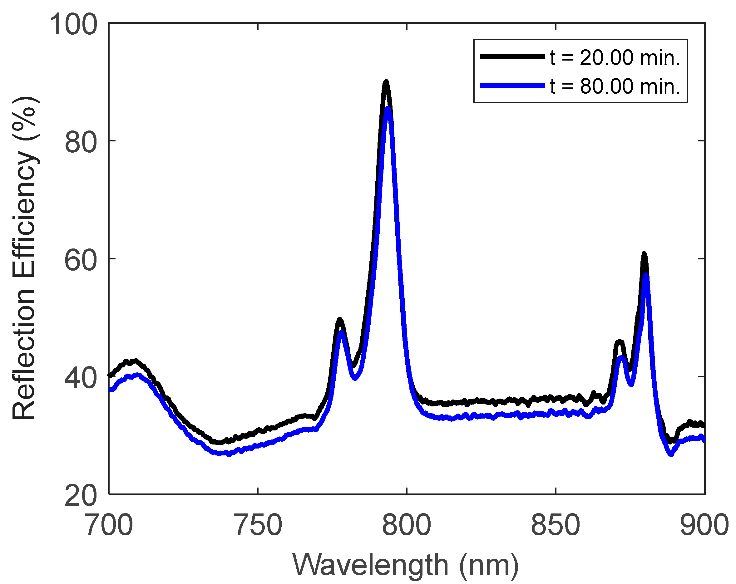
While the sensor is incubating in the yeast and PBS mixture, the resonance shifts are measured for the time interval from ~20 min to ~80 min, in ~10 s increments, and the changes in the biofilm and bulk are quantified. We have included the spectrum of the measurements at 20 min and 80 min in Figure 11.
4. Conclusions
Shifts in the wavelength of three resonant modes produced by a GMR sensor are used to simultaneously quantify the change in biolayer thickness, biolayer index of refraction, and bulk index of refraction. Extracting shifts in value for these three sensor variables using one spectral measurement, is an improvement in the field of biosensing. In past work, GMR sensors were used to monitor the bulk index of refraction and only one biolayer variable at a time.
The sensor used in this work is functionalized, with the protein Con A, for detection of Yarrowia yeast cells. During analyte accumulation, a set of three measured resonant wavelength shifts are used as inputs in a lookup table, and the outputs are three sensor variable value shifts: bulk index of refraction, biolayer thickness, and biolayer index of refraction. A label-free process that uses a single spectral measurement to determine changes in biolayer and bulk sensor variables is novel in practice. The multiparametric sensor, demonstrated via experiment and simulation in this work, can be used to quickly obtain detailed information about the sensor environment and the accumulation of a desired analyte over time. The key to our study is the use of a lookup table and an inversion algorithm to simultaneously monitor three sensor variables (two biolayer and one bulk) as biomolecules are captured on a sensor surface; this is a feat that has not been accomplished in past research—based on our review of the literature.
The simulation of the 2023 reflection spectra, each with a different variable value set, is an automated process using rigorous numerical models. This process can be applied to other sensors of interest and the number of variable value sets can be chosen freely, greatly exceeding the modest set count applied here. Implementing our inversion method with sensors that have a high sensitivity is expected to lead to a more accurate inversion; this would be important future work.
Author Contributions
Conceptualization, R.M. and J.A.B.-V.; methodology, J.A.B.-V.; writing-original draft preparation J.A.B.-V.; writing-review and editing, R.M.; funding acquisition, R.M. All authors have read and agreed to the published version of the manuscript.
Funding
This research was supported, in part, by the UT System Texas Nanoelectronics Research Superiority Award funded by the State of Texas Emerging Technology Fund as well as by the Texas Instruments Distinguished University Chair in Nanoelectronics endowment.
Institutional Review Board Statement
Not applicable.
Informed Consent Statement
Not applicable.
Data Availability Statement
The data presented in this study are available on request from the corresponding author.
Acknowledgments
The authors thank M. G. Abdallah, S. Das, and K. J. Lee for technical assistance. Parts of this research were conducted in the UT Arlington Shimadzu Institute Nanotechnology Research Center.
Conflicts of Interest
The authors declare no conflict of interest.
References
- Edmonds, P.; Cooney, J.J. Identification of Microorganisms Isolated from Jet Fuel Systems. Am. Soc. Microbiol. 1967, 15, 411–416. [Google Scholar] [CrossRef] [PubMed]
- Jung, C.M.; Broberg, C.; Giuliani, J.; Kirk, L.L.; Hanne, L.F. Characterization of JP-7 Jet Fuel Degradation by the Bacterium Nocardioides Luteus Strain BAFB. J. Basic Micro Biol. 2002, 42, 127–131. [Google Scholar] [CrossRef]
- Wawro, D.; Koulen, P.; Ding, Y.; Zimmerman, S.; Magnusson, R. Guided-mode resonance sensor system for early detection of ovarian cancer. In Proceedings of the Optical Diagnostics and Sensing X: Toward Point-of-Care Diagnostics, San Francisco, CA, USA, 25–26 January 2010; International Society for Optics and Photonics: Bellingham, WC, USA, 2010; Volume 7572, pp. 85–90. [Google Scholar] [CrossRef]
- Abdallah, M.G.; Buchanan-Vega, J.A.; Wenner, B.R.; Allen, J.W.; Allen, M.S.; Gimlin, S.; Weidanz, D.W.; Magnusson, R. Attachment and Detection of Biofouling Yeast Cells Using Biofunctionalized Resonant Sensor Modality. IEEE Sens. J. 2020, 21, 5995–6002. [Google Scholar] [CrossRef]
- Passman, F. Microbial contamination and its control in fuels and fuel systems since 1980—A review. Int. Biodeterior. Biodegrad. 2013, 81, 88–104. [Google Scholar] [CrossRef]
- Magnusson, R.; Wawro, D.; Zimmerman, S.; Ding, Y. Resonant Photonic Biosensors with Polarization-Based Multiparametric Discrimination in Each Channel. Sensors 2011, 11, 1476–1488. [Google Scholar] [CrossRef] [PubMed] [Green Version]
- Wawro, D.D.; Tibuleac, S.; Magnusson, R.; Liu, H. Optical fiber endface biosensor based on resonances in dielectric waveguide gratings. In Biomedical Diagnostic, Guidance, and Surgical-Assist Systems Ii; SPIE: San Jose, CA, USA, 2000; pp. 86–94. [Google Scholar] [CrossRef]
- Ding, Z.; Liu, P.; Chen, J.; Dai, D.; Shi, Y. On-chip simultaneous sensing of humidity and temperature with a dual-polarization silicon microring resonator. Opt. Express 2019, 27, 28649–28659. [Google Scholar] [CrossRef] [PubMed]
- Hossain, N.; Justice, J.; Lovera, P.; O’Riordan, A.; Corbett, B. Dual resonance approach to decoupling surface and bulk attributes in photonic crystal biosensor. Opt. Lett. 2014, 39, 6213–6216. [Google Scholar] [CrossRef] [PubMed]
- Cunningham, B.; Lin, B.; Qiu, J.; Li, P.; Pepper, J.; Hugh, B. A plastic colorimetric resonant optical biosensor for multiparallel detection of label-free biochemical interactions. Sens. Actuators B Chem. 2002, 85, 219–226. [Google Scholar] [CrossRef]
- Saleem, M.R.; Ali, R.; Honkanen, S.; Turunen, J. Bio-molecular sensors based on guided mode resonance filters. IOP Conf. Ser. Mater. Sci. Eng. 2016, 146, 012030. [Google Scholar] [CrossRef] [Green Version]
- Peterlinz, K.A.; Georgiadis, R. Two-Color Approach for Determination of Thickness and Dielectric Constant of thin Films Using Surface Plasmon Resonance Spectroscopy. Opt. Commun. 1996, 130, 260–266. [Google Scholar] [CrossRef]
- Johnston, K.S.; Karlsen, S.R.; Jung, C.C.; Yee, S.S. New analytical technique for characterization of thin films using surface plasmon resonance. Mater. Chem. Phys. 1995, 42, 242–246. [Google Scholar] [CrossRef]
- Adam, P.; Dostálek, J.; Homola, J. Multiple Surface Plasmon Spectroscopy for Study of Biomolecular Systems. Sens. Actuators B Chem. 2006, 113, 774–781. [Google Scholar] [CrossRef]
- de Bruijn, H.E.; Altenburg, B.S.; Kooyman, R.P.; Greve, J. Determination of thickness and dielectric constant of thin transparent dielectric layers using surface plasmon resonance. Opt. Commun. 1991, 82, 425–432. [Google Scholar] [CrossRef] [Green Version]
- Bahrami, F.; Aitchison, J.S.; Mojahedi, M. Multimode spectroscopy using dielectric grating coupled to a surface plasmon resonance sensor. Opt. Lett. 2014, 39, 3946–3949. [Google Scholar] [CrossRef] [PubMed]
- Shi, Q.; Zhao, J.; Liang, L. Two-dimensional photonic crystal slab biosensors using label free refractometric sensing schemes: A review. Prog. Quantum Electron. 2020, 77, 100298. [Google Scholar] [CrossRef]
- Das, S.; Samudrala, S.C.; Lee, K.J.; Abdallah, M.G.; Wenner, B.R.; Allen, J.W.; Allena, M.S.; Magnusson, R.; Vasilyev, M. SiN-Microring-Resonator-Based Optical Biosensor for Neuropeptide Y Detection. IEEE Photonics Technol. Lett. 2021, 33, 888–891. [Google Scholar] [CrossRef]
- Abdallah, M.G.; Buchanan-Vega, J.A.; Lee, K.J.; Wenner, B.R.; Allen, J.W.; Allen, M.S.; Gimlin, S.; Weidanz, D.W.; Magnusson, R. Quantification of Neuropeptide Y with Picomolar Sensitivity Enabled by Guided-Mode Resonance Biosensors. Sensors 2019, 20, 126. [Google Scholar] [CrossRef] [PubMed] [Green Version]
- Cooper, M.A. Current Biosensor Technologies in Drug Discovery. Drug Discov. 2006, 7, 68–82. [Google Scholar]
- Chandrasekar, R.; Lapin, Z.J.; Nichols, A.S.; Braun, R.M.; Fountain, A.W., III. Photonic Integrated Circuits for Department of Defense-Relevant Chemical and Biological Sensing Applications: State-of-the-Art and Furture Outlooks. Opt. Eng. 2019, 58, 020901. [Google Scholar] [CrossRef]
- Wang, W.; Qi, L. Light Management with Patterned Micro- and Nanostructure arrays for Photocatalysis, Photovoltaics and Optoelectronic and Optical Devices. Adv. Funct. Mater. 2019, 29, 1807275. [Google Scholar] [CrossRef]
- Guo, X. Surface plasmon resonance based biosensor technique: A review. J. Biophotonics 2012, 5, 483–501. [Google Scholar] [CrossRef] [PubMed]
- Chinowsky, T.M.; Yee, S.S. Quantifying the information content of surface plasmon resonance reflection spectra. Sens. Actuators B Chem. 1998, 51, 321–330. [Google Scholar] [CrossRef]
- Homola, J. Present and future of surface plasmon resonance biosensors. Anal. Bioanal. Chem. 2003, 377, 528–539. [Google Scholar] [CrossRef]
- Fannin, A.L.; Wenner, B.R.; Allen, J.W.; Allen, M.W.; Magnusson, R. Properties of Mixed Metal-Dielectric Nanogratings for Application in Resonant Absorption, Sensing, and Display. Opt. Eng. 2017, 56, 121905. [Google Scholar] [CrossRef]
- Magnusson, R.; Wang, S.S. New principle for optical filters. Appl. Phys. Lett. 1992, 61, 1022–1024. [Google Scholar] [CrossRef]
- Schmid, J.H.; Sinclair, W.; García, J.; Janz, S.; Lapointe, J.; Poitras, D.; Li, Y.; Mischki, T.; Lopinski, G.; Cheben, P.; et al. Silicon-on-insulator guided mode resonant grating for evanescent field molecular sensing. Opt. Express 2009, 17, 18371–18380. [Google Scholar] [CrossRef] [Green Version]
- Tibuleac, S.; Wawro, D.; Magnusson, R. Resonant diffractive structures integrating waveguide-gratings on optical fiber endfaces. In Proceedings of the 1999 IEEE LEOS Annual Meeting Conference Proceedings, LEOS’99, 12th Annual Meeting. IEEE Lasers and Electro-Optics Society 1999 Annual Meeting (Cat. No. 99CH37009), San Francisco, CA, USA, 8–11 November 1999. [Google Scholar] [CrossRef]
- Magnusson, R. The Complete Biosensor. Biosens. Bioelectron. 2013, 4, 1–2. [Google Scholar] [CrossRef]
- Moharam, M.G.; Gaylord, T.K.; Grann, E.B.; Pommet, D.A. Formulation for stable and efficient implementation of the rigorous coupled-wave analysis of binary gratings. J. Opt. Soc. Am. A 1995, 12, 1068–1076. [Google Scholar] [CrossRef]
- RSoft Photonic Device Tools (Diffract MOD Synopsys). Available online: https://www.synopsys.com/photonic-solutions (accessed on 17 August 2022).
- Dusane, D.H.; Nancharaiah, Y.V.; Venugopalan, A.P.; Kumar, A.R.; Zinjarde, S.S. Biofilm Formation by a Biotechnologicallly Important Tropical Marine Yeast Isolate, Yarrowia Lipolytica NCIM 3589. Water Sci. Technol. 2008, 58, 1221–1229. [Google Scholar] [CrossRef]
- Tkacz, J.S.; Cybulska, E.B.; Lampen, J.O. Specific Staining of Wall Mannan in Yeast Cells with Fluorescein-Conjugated Concanavalin A. J. Bacteriol. 1971, 105, 1–5. [Google Scholar] [CrossRef]
- U.S. Food Drug Administration. Available online: https://www.fda.gov/regulatory-information/search-fda-guidance-documents/q2b-validation-analytical-procedures-methodology (accessed on 4 December 2020).
Figure 1.
(a) The sensor used in this work consists of a silicon nitride (Si3N4) grating and homogeneous layer on a quartz substrate. The orange horizontal line at the substrate/homogeneous layer interface represents a light source directed upward. The grating parameters are as follows: fill factor (F) = 0.42, grating depth (dg) = 260 nm, homogeneous layer depth (dh) = 500 nm, and period (Λ) = 500 nm. (b) The RCWA simulated zero-order TM reflection spectrum from 700 to 900 nm for homogeneous layer thicknesses 0, 300, 400, and 500 nm. (c) The same for the TE spectrum. TE polarization has the electric field vector normal to the plane of incidence, whereas TM polarization has the magnetic field vector normal to the plane of incidence.

Figure 2.
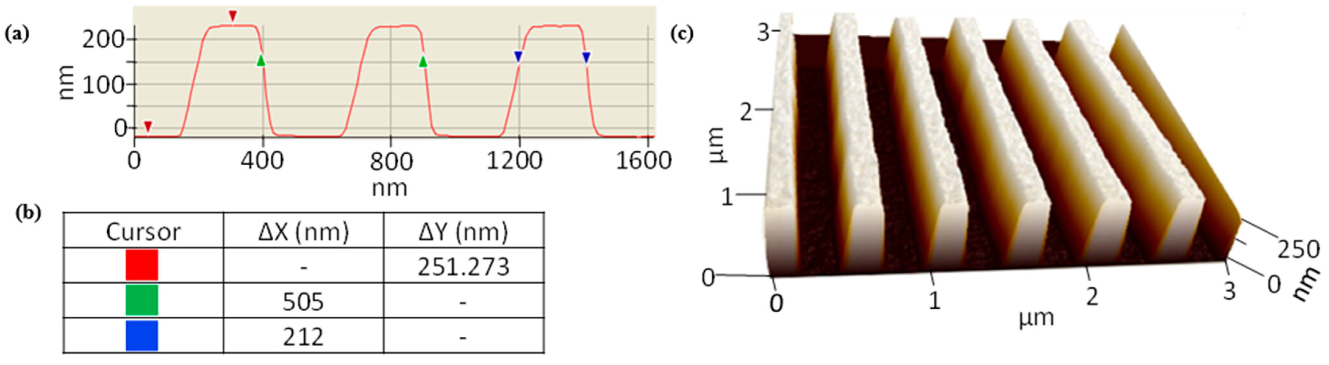
(a) An atomic force microscope (AFM) generated profile of the sensor grating. The colored arrows indicate the positions used to measure grating depth (red), period (green), and fill factor (blue). (b) A table with horizontal (ΔX) and vertical (ΔY) measurements based upon the colored arrow locations in (a): red indicates the grating depth, green indicates the period, and blue indicates the grating width. The cursor locations indicate the grating depth (dg = 251 nm), period (Λ = 505 nm), and fill factor (F = 0.42). The fabricated parameters are close to the design parameters which are dg = 260 nm, Λ = 500 nm, and F = 0.42. (c) An AFM generated 3D rendering of the sensor grating.
Figure 2.
(a) An atomic force microscope (AFM) generated profile of the sensor grating. The colored arrows indicate the positions used to measure grating depth (red), period (green), and fill factor (blue). (b) A table with horizontal (ΔX) and vertical (ΔY) measurements based upon the colored arrow locations in (a): red indicates the grating depth, green indicates the period, and blue indicates the grating width. The cursor locations indicate the grating depth (dg = 251 nm), period (Λ = 505 nm), and fill factor (F = 0.42). The fabricated parameters are close to the design parameters which are dg = 260 nm, Λ = 500 nm, and F = 0.42. (c) An AFM generated 3D rendering of the sensor grating.

Figure 3.
Schematic of the sensor layout. The broadband light from the source is sent through the fiber optic cable, the converging lens, and the aperture. The light then interacts with the GMR sensor and travels back through the optical elements to reach the spectrometer.
Figure 3.
Schematic of the sensor layout. The broadband light from the source is sent through the fiber optic cable, the converging lens, and the aperture. The light then interacts with the GMR sensor and travels back through the optical elements to reach the spectrometer.

Figure 4.
Simulated bulk index of refraction shifts and the resultant resonant wavelength shifts for the TM and TE resonant modes: the biolayer thickness for these simulations is 0 nm. Each resonant mode is plotted with its best fit line of corresponding color.
Figure 4.
Simulated bulk index of refraction shifts and the resultant resonant wavelength shifts for the TM and TE resonant modes: the biolayer thickness for these simulations is 0 nm. Each resonant mode is plotted with its best fit line of corresponding color.

Figure 5.
A plot of the simulated (a) TM0 resonance wavelength shifts for a given biolayer index of refraction and biolayer thickness for the biosensor shown in Figure 1a; each sheet of simulation data represents a different value of bulk index of refraction (buffer) as indicated in the legend. This plot is also produced for the (b) TM1 and (c) TE1 modes of light.

Figure 6.
Measured unpolarized reflection spectrum of our bare GMR biosensor, with deionized (DI) water background, whose AFM is shown in Figure 2c. From lowest to highest wavelength, the peaks are due to TM1, TE1, TM0, and TE0 resonant modes as labeled on the figure.
Figure 6.
Measured unpolarized reflection spectrum of our bare GMR biosensor, with deionized (DI) water background, whose AFM is shown in Figure 2c. From lowest to highest wavelength, the peaks are due to TM1, TE1, TM0, and TE0 resonant modes as labeled on the figure.

Figure 7.
Experimentally measured reflection spectrum during sensor incubation in a Con A and PBS solution (1 mg/mL). The spectra displayed are at beginning incubation time 0.17 min and at final incubation time 80.00 min.
Figure 7.
Experimentally measured reflection spectrum during sensor incubation in a Con A and PBS solution (1 mg/mL). The spectra displayed are at beginning incubation time 0.17 min and at final incubation time 80.00 min.

Figure 8.
Experimentally measured resonance wavelength shifts during sensor incubation in a Con A and PBS solution (1 mg/mL). The TM0, TM1, and TE1 modes are labeled in the legend as black, blue, and red, respectively.
Figure 8.
Experimentally measured resonance wavelength shifts during sensor incubation in a Con A and PBS solution (1 mg/mL). The TM0, TM1, and TE1 modes are labeled in the legend as black, blue, and red, respectively.

Figure 9.
Changes in the (a) biolayer index of refraction and (b) biolayer thickness during the incubation of the sensor in Con A. During this process, the change in the bulk refractive index (Δnbulk) is calculated to be 0 RIU.
Figure 9.
Changes in the (a) biolayer index of refraction and (b) biolayer thickness during the incubation of the sensor in Con A. During this process, the change in the bulk refractive index (Δnbulk) is calculated to be 0 RIU.

Figure 10.
Scaled GMR sensor response from a series dilution of yeast cells in suspension with PBS. This data is based on our past work published in Abdallah et al. [4].
Figure 10.
Scaled GMR sensor response from a series dilution of yeast cells in suspension with PBS. This data is based on our past work published in Abdallah et al. [4].

Figure 11.
Experimentally measured reflection spectrum during sensor incubation in a yeast and PBS solution ( cells/mL). The spectra displayed are at incubation times 20.00 min and at 80.00 min.
Figure 11.
Experimentally measured reflection spectrum during sensor incubation in a yeast and PBS solution ( cells/mL). The spectra displayed are at incubation times 20.00 min and at 80.00 min.

Figure 12.
Resonance wavelength shifts while the sensor is incubated in a yeast and PBS solution ( cells/mL). The TM0, TM1, and TE1 modes are labeled in the legend as black, blue, and red, respectively.
Figure 12.
Resonance wavelength shifts while the sensor is incubated in a yeast and PBS solution ( cells/mL). The TM0, TM1, and TE1 modes are labeled in the legend as black, blue, and red, respectively.

Figure 13.
Changes in the (a) biolayer refractive index and (b) biolayer thickness during the incubation of the sensor in yeast. During this process, the change in the bulk refractive index (Δnbulk) is calculated to be 0 RIU.
Figure 13.
Changes in the (a) biolayer refractive index and (b) biolayer thickness during the incubation of the sensor in yeast. During this process, the change in the bulk refractive index (Δnbulk) is calculated to be 0 RIU.


Table 1.
Simulation Input and Algorithm Output.
| Simulation Input | Algorithm Output | ||||
|---|---|---|---|---|---|
| Δnbio (RIU) | Δdbio (nm) | Δnbulk (RIU) | Δnbio (RIU) | Δdbio (nm) | Δnbulk (RIU) |
| 0.010 | 2.0 | 0 | 0.009 | 2.0 | 0 |
| 0.058 | 11.0 | 0 | 0.062 | 11.0 | 0 |
| 0.086 | 15.5 | 0 | 0.087 | 15.5 | 0 |
| 0.086 | 20.0 | 0 | 0.090 | 19.0 | 0 |
| 0.058 | 2.0 | 0.048 | 0.057 | 2.0 | 0.048 |
| 0.077 | 11.0 | 0.048 | 0.075 | 12.5 | 0.048 |
| 0.010 | 15.5 | 0.048 | 0.012 | 17.0 | 0.048 |
| 0.010 | 20.0 | 0.048 | 0.009 | 18.5 | 0.048 |
| 0.086 | 2.0 | 0.096 | 0.087 | 2.0 | 0.096 |
| 0.038 | 11.0 | 0.096 | 0.034 | 11.0 | 0.096 |
| 0.010 | 15.5 | 0.096 | 0.009 | 15.5 | 0.096 |
| 0.010 | 20.0 | 0.096 | 0.006 | 19.0 | 0.096 |
Table 2.
Experimental Input and Algorithm Output for Con A Detection.
| Experimental Input | Algorithm Output | ||||
|---|---|---|---|---|---|
| Δλ TM0 (nm) | Δλ TM1 (nm) | Δλ TE1 (nm) | Δnbio (RIU) | Δdbio (nm) | Δnbulk (RIU) |
| 0.074 | 0.18 | 0.058 | 0.047 | 7.2 | 0 |
Table 3.
Experimental Input and Algorithm Output for Yeast.
| Experimental Input | Algorithm Output | ||||
|---|---|---|---|---|---|
| Δλ TM0 (nm) | Δλ TM1 (nm) | Δλ TE1 (nm) | Δnbio (RIU) | Δdbio (nm) | Δnbio (RIU) |
| 0.051 | 0.061 | 0.016 | 0.02 | 6.7 | 0 |
Publisher’s Note: MDPI stays neutral with regard to jurisdictional claims in published maps and institutional affiliations. |
© 2022 by the authors. Licensee MDPI, Basel, Switzerland. This article is an open access article distributed under the terms and conditions of the Creative Commons Attribution (CC BY) license (https://creativecommons.org/licenses/by/4.0/).
Share and Cite
MDPI and ACS Style
Buchanan-Vega, J.A.; Magnusson, R. Multiparametric Guided-Mode Resonance Biosensor Monitoring Bulk and Surface-Film Variations. Chemosensors 2022, 10, 541. https://doi.org/10.3390/chemosensors10120541
AMA Style
Buchanan-Vega JA, Magnusson R. Multiparametric Guided-Mode Resonance Biosensor Monitoring Bulk and Surface-Film Variations. Chemosensors. 2022; 10(12):541. https://doi.org/10.3390/chemosensors10120541
Chicago/Turabian StyleBuchanan-Vega, Joseph A., and Robert Magnusson. 2022. "Multiparametric Guided-Mode Resonance Biosensor Monitoring Bulk and Surface-Film Variations" Chemosensors 10, no. 12: 541. https://doi.org/10.3390/chemosensors10120541
Note that from the first issue of 2016, this journal uses article numbers instead of page numbers. See further details here.