Dynamic Analysis of a Particle Motion System

1
Department of Mathematics and Sciences, Hebei Institute of Architecture and Civil Engineering, Zhangjiakou 075000, Hebei Province, China
2
School of Mathematics and Statistics, Beijing Institute of Technology, Beijing 100081, China
*
Author to whom correspondence should be addressed.
Mathematics 2019, 7(1), 7; https://doi.org/10.3390/math7010007
Submission received: 22 November 2018
/
Revised: 15 December 2018
/
Accepted: 16 December 2018
/
Published: 21 December 2018
Abstract
:This paper formulates a new particle motion system. The dynamic behaviors of the system are studied including the continuous dependence on initial conditions of the system’s solution, the equilibrium stability, Hopf bifurcation at the equilibrium point, etc. This shows the rich dynamic behaviors of the system, including the supercritical Hopf bifurcations, subcritical Hopf bifurcations, and chaotic attractors. Numerical simulations are carried out to verify theoretical analyses and to exhibit the rich dynamic behaviors.
1. Introduction
There are some scholars who have studied the dynamic behaviors of particle motion. The results show that particle motion is a complex dynamic behavior in some case, such as chaotic motion. For instance, Abbott N. L. investigated the diffusion of a colloidal particle in a liquid crystalline solvent [1]. Chen C. and his colleague studied the chaotic particle dynamics in free-electron lasers and obtained that the particle motion becomes chaotic on a time scale. Here, the time scale is the characteristic time scale for radial-gradient-induced changes in the particle orbits, which is shown to be of the order of the beam transit time through a few wiggler periods [2]. Research showed that the chaos of a particle probing the black hole horizon had a universal upper bound for the Lyapunov exponent [3]. Since chaos began to be studied, it has been a common belief that understanding and utilizing the rich dynamics of a nonlinear system have an important impact on modern technology. Therefore, it also promotes the study of chaos, and some useful results have been obtained. For example, Sprott J. C. and Xiong A. [4] presented a method for classifying basins of attraction and quantifying their size for any dissipative dynamical system, and the results were useful to describe the basin of attraction and quantifying its shape and size for both theoretical and practical reasons. By using the Pynamical software package, Boeing G. [5] investigated visualization methods of nonlinear dynamical systems’ behavior and indicated that these methods can help researchers discover, examine, and understand the behaviors of nonlinear dynamical systems, including bifurcations, the path to chaos, fractals, and strange attractors. Bradley E. and Kantz H. [6] illustrated that the results of nonlinear time-series analysis can be helpful in understanding, characterizing, and predicting dynamical systems. In fact, chaos has many manifestations in many different situations [7]. Meanwhile, many systems will appear with multiple equilibrium points under some parameter conditions, and the increase of the equilibrium points or multi-equilibrium points may lead to richer dynamic behaviors of the system [8,9,10]. For these reasons, we will formulate a particle motion model under external force and discuss the Hopf bifurcation and chaotic behaviors of the system.
In this paper, we will formulate a new model for particle motion and the stability of equilibrium points. The continuous dependence on initial conditions of the system’s solution and Hopf bifurcation are investigated in Section 2. To further study the complex dynamic behaviors of particle motion, simulations including Lyapunov exponents, Poincaré maps and phase portraits of the chaotic attractor for the system are given in Section 3. A summary of our results and further discussion are presented in Section 4.
2. Model
There are rich dynamic behaviors in some cases, such as in sheared suspensions [11], in creeping flow [12], and around a weakly-magnetized Schwarzschild black hole [13]. This shows that the particle motion becomes complex because of the existence of external force, and the particle system has different dynamic behaviors under different external forces [14,15,16]. Here, we assume that a particle with unit mass is moving on a horizontal smooth plane , and the forces on the particle in p and q direction are and , respectively, where:
, , , and are all positive parameters. The dot expresses the derivative with respect to the time variable t. Then, the particle motion equations are described by:
2.1. Symmetry and Dissipation
Obviously, System (1) is symmetric with coordinate transformations:
The divergence of (1) is:
Thus, the system is dissipative. This indicates that the volume element as , then all the trajectories of the system (1) are ultimately in an attractor.
2.2. Existence and Uniqueness of the Solution
We first rewrite the system (1) as follows:
where:
, .
Let
and . The existence and uniqueness of the solution are studied in the region where . The solution of (2) with initial conditions is:
where:
Next, we denote the right-hand side of (3) by , then:
here:
Therefore,
The supremum norm is defined for the class of continuous function by:
and for a matrix , which is defined by . Thus, we obtain:
where:
The following theorem is obtained.
Theorem 1.
The sufficient condition for the existence and uniqueness of the solution of (1) with initial conditions in the region is .
2.3. Continuous Dependence on Initial Conditions
Based on the results in Section 2.1, we have:
where:
and are all the initial conditions to (2) and . Under the condition of Theorem 1, the following inequality is obtained:
hence . In conclusion, , such that implies that .
Theorem 2.
There is continuous dependence on the initial conditions of the solution of (1) under the condition of Theorem 1.
2.4. Equilibrium and Stability
It is easy to visualize that (1) always has three equilibrium points, i.e.,
When , (1) has equilibria as follows:
where:
By calculations, the characteristic equations at equilibrium points are obtained as follows:
Obviously, , , and have roots with positive real parts, and , , and are unstable. In the following, we will discuss the bifurcations at the rest of the equilibrium points.
2.5. Hopf Bifurcation
In this subsection, the Hopf bifurcation of System (1) is investigated by using the theories in [10].
When has a pair of pure imaginary roots , becomes:
then we get:
By calculations,
Therefore, the eigenvalues of Jacobian matrix at are:
By straightforward computations, we obtain the eigenvectors with respect to , i.e.,
where:
Let , and denote the real and imaginary parts of , then:
For , the eigenvectors are obtained:
Next, we use the following transformation:
Then, the system (1) becomes:
where the items can be seen in Appendix A.
According to the center manifold theorem [17], there exists a center manifold for (1) as follows:
for sufficiently small . We assume that:
where the items can be seen in Appendix A. Then:
Therefore, it is obtained that:
where the items and can be seen in Appendix A.
Therefore, applying the method in [17], we can compute the first-order fine focus as follows:
where the items and can be seen in Appendix A.
Theorem 3.
The supercritical Hopf bifurcation of the system (1) occurs if , and the subcritical Hopf bifurcation occurs if .
The same approach can be used to study the Hopf bifurcation at the other equilibrium .
3. Simulation
In this section, the example of Hopf bifurcations for the system is given, and it shows that chaotic phenomena occur in the system with some parameter values. Firstly, we fix the parameters as follows:
The eigenvalues of the Jacobian matrix at the equilibrium point are and , and the Hopf bifurcation occurs in the system (1). Based on Theorem 3, we get , then the Hopf bifurcation at the equilibrium point of system (1) is non-degenerate, and the bifurcating periodic solution is stable. Because of the symmetry of the system (1), the same type of Hopf bifurcation occurs at the equilibrium . The phase diagrams in the p-u plane and the q-v plane of system (1) with initial values are given in Figure 1 and Figure 2, respectively. It is shown that the system has a stable limit cycle around the equilibrium point. Moreover, the eigenvalues of the Jacobian matrix at the equilibria , , and are:
and , respectively. Thus, is a stable-focus point with a four-dimensional unstable manifold, and , are all stable-focus points with a three-dimensional stable manifold and a one-dimensional unstable manifold.
Next, we assume the parameters as follows:
In this case, the system (1) has nine equilibrium points. Table 1 indicates the eigenvalues of the corresponding Jacobian matrix and the equilibria type and shows the unstable manifold and stable manifold at the equilibrium points of the particle motion system.
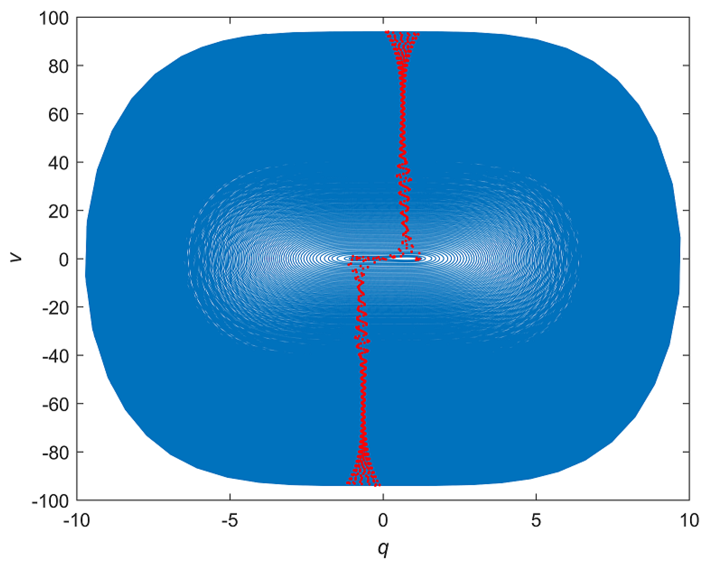
It has been long supposed that the existence of chaotic behavior in the microscopic motions is responsible for their equilibrium and non-equilibrium properties [18], and the increase of the equilibrium points or multi-equilibrium points may lead to abundant dynamic behaviors of the system [8,9,10]. From the above results, it is shown that the system (1) has multi-equilibrium points with a stable manifold and an unstable manifold. Therefore, the particle motion system has rich dynamic behaviors. The Lyapunov exponents are , , , and by using the method in [19]; thus, the system (1) is chaotic. In addition, the chaotic phenomena can also be reflected by the Poincaré maps [20]. Therefore, the chaotic attractor in the plane of System (1) with parameters , , , and initial values is shown in Figure 3a, and the Poincaré mapping on the section hyperplane is given in Figure 3b. The chaotic attractor in the plane of System (1) with parameters , , , and initial values is shown in Figure 4a, and the Poincaré mapping on the section hyperplane is given in Figure 4b. Here, the Runge–Kutta method of order four is employed with the time step of from to . This shows that the particle motion trajectories and the velocities of the particle in both directions are complex and the particle motion chaotic. Hence, the particle motion system shows chaotic behavior. To further illustrate the strange attractors of System (1), Figure 5 and Figure 6 show the chaos phase portrait of and and the corresponding Poincaré map by taking the same parameters and initial values as Figure 3.
4. Conclusions
In this paper, a particle motion model is formulated by introducing external forces. The dynamic behaviors of the system are investigated, including the symmetry, the existence and uniqueness of the solution, and the continuous dependence on initial conditions. The range of the parameter where the solution of the system shows continuous dependence on initial conditions can be determined from Theorems 1 and 2. Consequently, the range of parameter values of the system where the system does not exhibit chaotic behavior can be determined in theory. The results provide great help in controlling the dynamic behavior of the particle motion system. By using the center manifold theorem and simulations, the Hopf bifurcations at the equilibrium and chaotic behavior are studied. This illustrates that the particle motion system has rich dynamic phenomena and also indicates the influence of the external force on the particle motion trajectories. Compared to [21,22], different results are obtained, such as Theorems 1 and 2, and the dynamic behaviors of the particle motion system are investigated by applying different methods such as the method in [17] and the Poincaré section. These results are helpful for further understanding the state of particle motion under external force. How to effectively control the chaotic behavior and bifurcation phenomena of particle motion will be our next research direction.
Author Contributions
All authors have equally contributed to this work. All authors revised and edited the final version of the manuscript.
Funding
The project was supported by the Youth Science Foundations of Education Department of Hebei Province (No. QN2016265), the Hebei Special Foundation “333 talent project” (No. A2016001123), and the Scientific Research Funds of Hebei Institute of Architecture and Civil Engineering (Nos. 2016XJJQN03, 2016XJJYB05).
Acknowledgments
The authors would like to thank the editor and referees for their positive and constructive comments, which are all valuable and very helpful for improving this paper.
Conflicts of Interest
The authors declare no conflict of interest.
Appendix A
(1) Expressions of in Section 2.5:
where:
, ,
, ,
,
,
,
,
, ,
,
, ,
,
,
.
,
,
,
.
(3) Expressions of and in Section 2.5:
(4) Expressions of and in Section 2.5:
References
- Abbott, N.L. Colloid Science Collides with Liquid Crystals. Science 2013, 342, 1326–1327. [Google Scholar] [CrossRef] [PubMed]
- Chen, C.; Davidson, R.C. Chaotic particle dynamics in free-electron lasers. Phys. Rev. A 1991, 43, 5541. [Google Scholar] [CrossRef] [PubMed]
- Hashimoto, K.; Tanahashi, N. Universality in chaos of particle motion near black hole horizon. Phys. Rev. D 2017, 95, 024007. [Google Scholar] [CrossRef] [Green Version]
- Sprott, J.C.; Xiong, A. Classifying and quantifying basins of attraction. Chaos 2015, 25, 22–30. [Google Scholar] [CrossRef] [PubMed]
- Boeing, G. Visual analysis of nonlinear dynamical systems: Chaos, fractals, self-similarity and the limits of prediction. System 2016, 4, 37–54. [Google Scholar] [CrossRef]
- Bradley, E.; Kantz, H. Nonlinear time-series analysis revisited. Chaos 2015, 25, 097610. [Google Scholar] [CrossRef] [PubMed] [Green Version]
- Sander, E.; Yorke, J.A. The Many Facets of Chaos. Int. J. Bifurcat. Chaos 2015, 25, 1530011. [Google Scholar] [CrossRef]
- Yuan, F.; Wang, G.; Wang, X. Extreme multistability in a memristor-based multi-scroll hyperchaotic system. Chaos 2016, 26, 507–519. [Google Scholar] [CrossRef]
- Zhou, P.; Yang, F. Hyperchaos, chaos, and horseshoe in a 4D nonlinear system with an infinite number of equilibrium points. Nonlinear Dyn. 2013, 76, 473–480. [Google Scholar] [CrossRef]
- Liu, X.; Shen, X.S.; Zhang, H. Multi-scroll chaotic and hyperchaotic attractors generated from chen system. Int. J. Bifurcat. Chaos 2012, 22, 1250033. [Google Scholar] [CrossRef]
- Pine, D.J.; Gollub, J.P.; Brady, J.F.; Leshansky, A.M. Chaos and threshold for irreversibility in sheared suspensions. Nature 2005, 438, 997–1000. [Google Scholar] [CrossRef] [PubMed] [Green Version]
- Enkeleida, L.; Petia, M.V. Periodic and chaotic orbits of plane-confined micro-rotors in creeping flows. J. Nonlinear Sci. 2015, 25, 1111–1123. [Google Scholar]
- AlZahrani, A.M.; Frolov, V.P.; Shoom, A.A. Critical escape velocity for a charged particle moving around a weakly magnetized Schwarzschild black hole. Phys. Rev. D 2013, 87, 084043. [Google Scholar] [CrossRef]
- Kuwana, C.M.; Oliveiraz, J.A.; Leonel, E.D. A family of dissipative two-dimensional mappings: Chaotic, regular and steady state dynamics investigation. Phys. A 2014, 395, 458–465. [Google Scholar] [CrossRef]
- Oliveira, D.F.; Leonel, E.D. Parameter space for a dissipative Fermi-Ulam model. New J. Phys. 2011, 13, 123012. [Google Scholar] [CrossRef]
- Costa, D.R. A dissipative Fermi-Ulam model under two different kinds of dissipation. Commun. Nonlinear Sci. 2015, 22, 1263–1274. [Google Scholar] [CrossRef]
- Carr, J. Applications of Centre Manifold Theory; Springer: New York, NY, USA, 1981. [Google Scholar]
- Gaspard, P.; Briggs, M.E.; Francis, M.K.; Sengers, J.V.; Gammon, R.W.; Dorfman, J.R.; Calabrese, R.V. Experimental evidence for microscopic chaos. Nature 1998, 6696, 865–868. [Google Scholar] [CrossRef]
- Wolf, A.; Swift, J.B.; Swinney, H.L.; Vastano, J.A. Determining Lyapunov exponents from a time series. Physica D 1985, 16, 285–317. [Google Scholar] [CrossRef] [Green Version]
- Awrejcewicz, J.; Olejnik, P. Stick-slip dynamics of a two-degree-of-freedom system. Int. J. Bifurcat. Chaos 2013, 13, 843–861. [Google Scholar] [CrossRef]
- Li, J.; Wu, H.; Mei, F. Dynamic analysis for the hyperchaotic system with nonholonomic constraints. Nonlinear Dyn. 2017, 90, 2557–2569. [Google Scholar] [CrossRef]
- Chang, C.; Ge, Z. Complete identification of chaos of nonlinear nonholonomic systems. Nonlinear Dyn. 2010, 60, 551–559. [Google Scholar] [CrossRef]
Figure 1.
The phase diagram in the p-u plane.
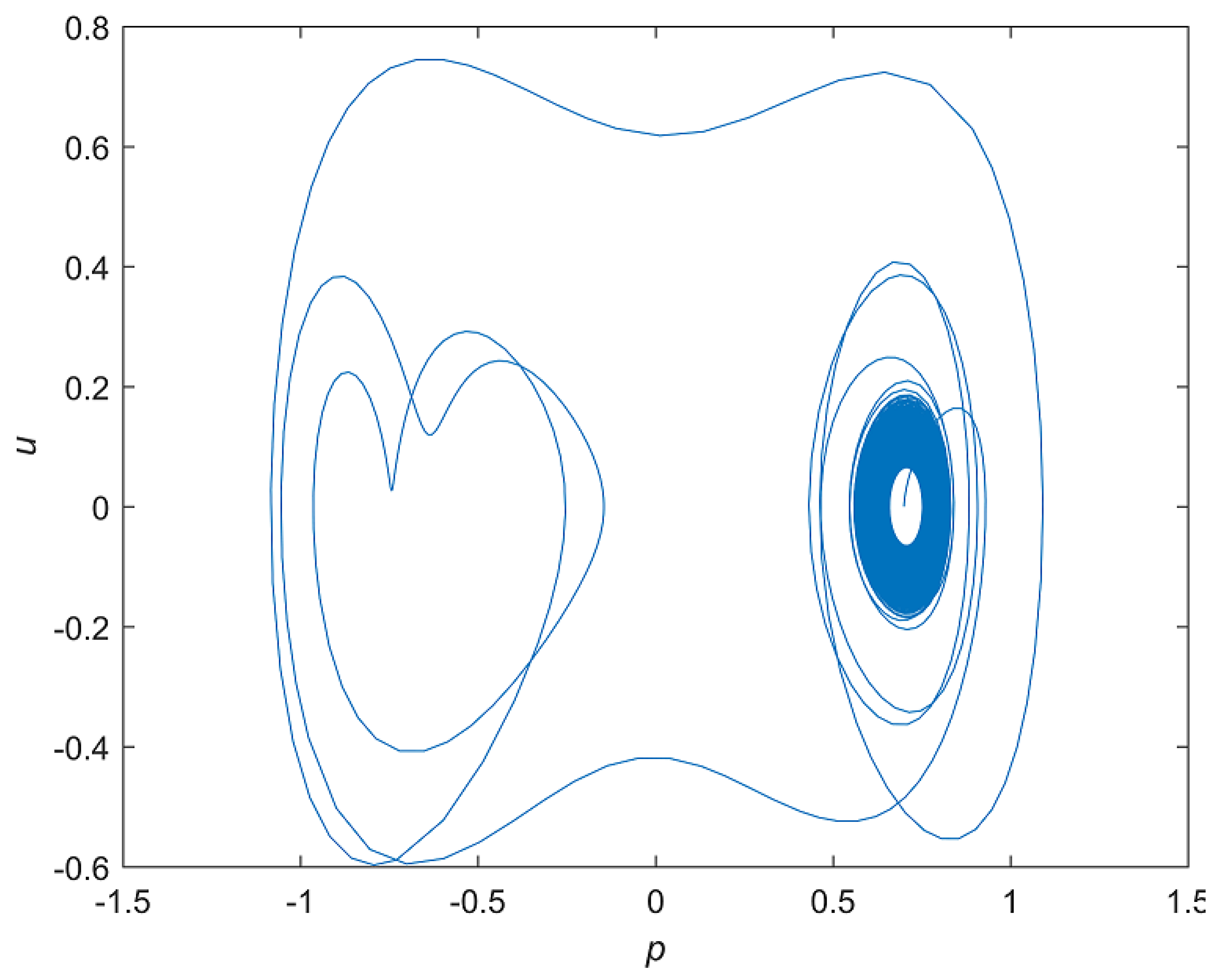
Figure 2.
The phase diagram in the q-v plane.
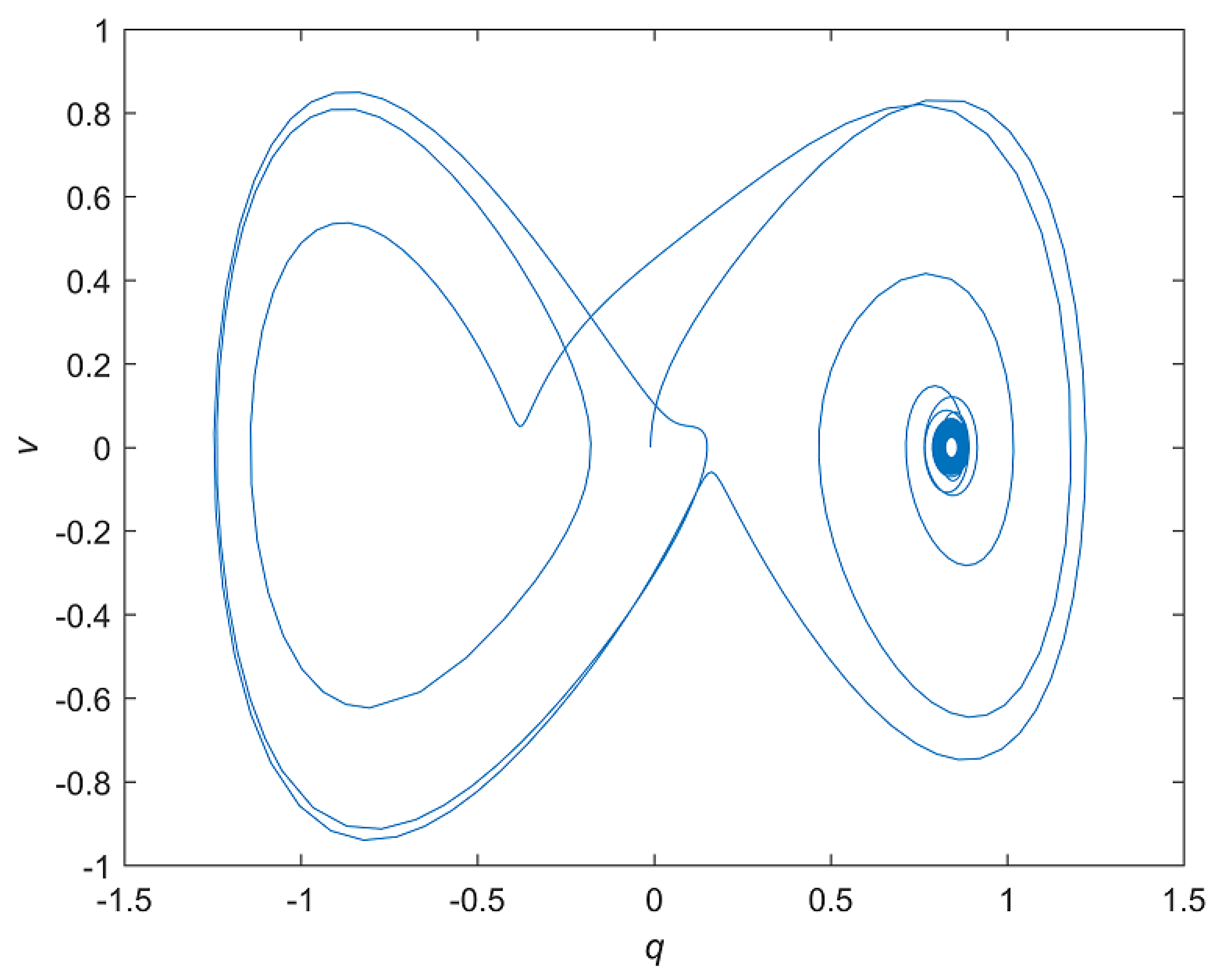
Figure 3.
(a) The chaotic attractor in the p-q plane; (b) The Poincaré mapping on the section .
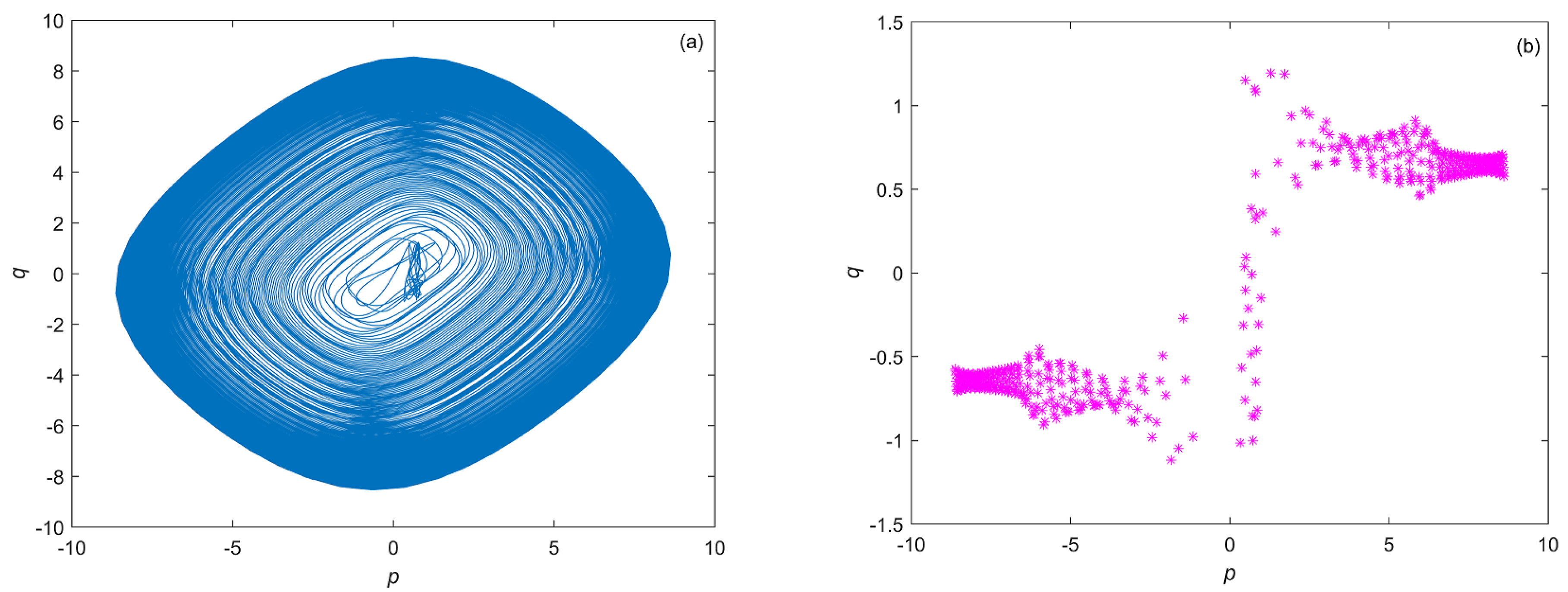
Figure 4.
(a) The chaotic attractor in the u-v plane; (b) The Poincaré mapping on the section .

Figure 5.
p-u phase portrait and the corresponding Poincaré map (red points) on the section .
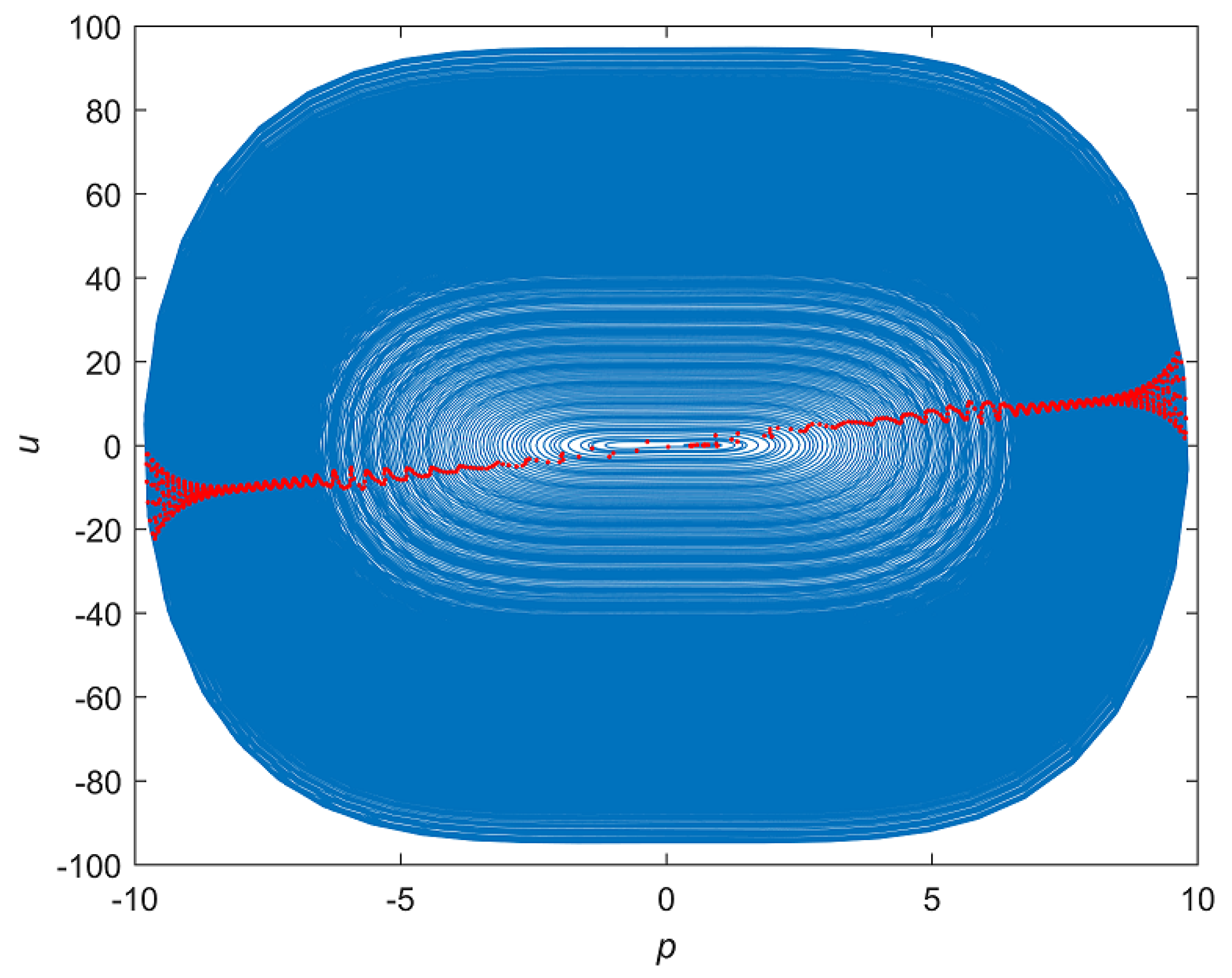
Figure 6.
q-v phase portrait and the corresponding Poincaré map (red points) on the section .

Table 1.
The eigenvalues of the corresponding Jacobian matrix and the equilibria type.
| Equilibrium Points | Eigenvalues of the Jacobian Matrix | Equilibria Type |
|---|---|---|
| , , | saddle-focus point | |
| , , | saddle-focus point | |
| , , | saddle-focus point | |
| , , | saddle-focus point | |
| , , | saddle-focus point | |
| , | focus point | |
| , | focus point | |
| , | focus point | |
| , | focus point |
© 2018 by the authors. Licensee MDPI, Basel, Switzerland. This article is an open access article distributed under the terms and conditions of the Creative Commons Attribution (CC BY) license (http://creativecommons.org/licenses/by/4.0/).
Share and Cite
MDPI and ACS Style
Cui, N.; Li, J. Dynamic Analysis of a Particle Motion System. Mathematics 2019, 7, 7. https://doi.org/10.3390/math7010007
AMA Style
Cui N, Li J. Dynamic Analysis of a Particle Motion System. Mathematics. 2019; 7(1):7. https://doi.org/10.3390/math7010007
Chicago/Turabian StyleCui, Ning, and Junhong Li. 2019. "Dynamic Analysis of a Particle Motion System" Mathematics 7, no. 1: 7. https://doi.org/10.3390/math7010007
Note that from the first issue of 2016, this journal uses article numbers instead of page numbers. See further details here.