SPGD: Search Party Gradient Descent Algorithm, a Simple Gradient-Based Parallel Algorithm for Bound-Constrained Optimization

Abstract

Nature-inspired metaheuristic algorithms remain a strong trend in optimization. Human-inspired optimization algorithms should be more intuitive and relatable. This paper proposes a novel optimization algorithm inspired by a human search party. We hypothesize the behavioral model of a search party searching for a treasure. Motivated by the search party’s behavior, we abstract the “Divide, Conquer, Assemble” (DCA) approach. The DCA approach allows us to parallelize the traditional gradient descent algorithm in a strikingly simple manner. Essentially, multiple gradient descent instances with different learning rates are run parallelly, periodically sharing information. We call it the search party gradient descent (SPGD) algorithm. Experiments performed on a diverse set of classical benchmark functions show that our algorithm is good at optimizing. We believe our algorithm’s apparent lack of complexity will equip researchers to solve problems efficiently. We compare the proposed algorithm with SciPy’s optimize library and it is found to be competent with it.

1. Introduction

Optimization is an evergreen field of engineering. Domains like marketing, economics, science, and finance are full of optimization problems (OPs). An arsenal of powerful algorithms is available for optimization, but the search for a better algorithm seems never to end. There are two main types of optimization algorithms: exact and heuristic/stochastic methods [1]. Stochastic methods are preferred over exact methods as they are approximate methods and can provide near-optimal solutions with less computational effort [1]. In real-world problems like machine learning, it is sufficient to have near-optimal solutions to achieve desired results, and avoid overfitting. In this paper, we consider OPs subject to simple bounds on the variables. The bound-constrained optimization (BCO) problem is to minimize a single objective function of the D dimension subjected to simple bounds on the variables [2]:

$$\mathrm{Min}f\left(\overline{X}\right)$$

(1)

where, $f$: ${ℝ}^D\to ℝ$ is a real valued function; $\overline{X}=\left(x_1,x_2,\dots ,x_d\right) €{ℝ}^D$ is a D dimensional vector such that,

$$\overline{LB}\le \overline{X}\le \overline{UB}$$

(2)

Vectors $\overline{LB}$ and $\overline{UB}$ represent lower and upper bound on $\overline{X}$ [2].

Many novel approaches are being introduced in the literature for optimization. Nature-inspired algorithms, especially evolutionary algorithms, are popular stochastic optimization methods. Most of these algorithms are complex and are often used by researchers as black-box optimizers ignoring their internal working [3]. A simple and robust optimization algorithm, which is easy to understand, can serve as a great quick start for researchers to tackle OPs with confidence.

Genetic algorithms (GA), particle swarm optimization (PSO), and differential evolution are well-established evolutionary algorithms. Evolutionary algorithms search from multiple points and hence are inherently parallel [1]. Several modifications and hybridization to the evolutionary algorithms have also been reported [4]. Gradient-based PSO is one such hybrid optimization algorithm that combines stochastic PSO for search diversification and deterministic gradient descent (GD) to intensify the search. The authors of [5] present a hybridization approach that combines deterministic local search optimization methods like Nelder-mead with simulated annealing, a metaheuristic global OP algorithm. The gradient-based genetic algorithm [1] is another similar hybrid algorithm that uses GD for exploitation and GA for exploration, specifically for constrained optimization. Since GD is highly efficient in local optimization, it is hybridized commonly with a global optimization algorithm (generally gradient-free), and they are designed to complement each other. Our proposed algorithm also uses GD for exploitation and an exploration scheme based on the decaying epsilon greedy strategy from the multi-armed bandit (MAB) problem [6]. We run a fixed number of parallel GD instances from multiple starting points in the hope of finding the global optimum. After a fixed number of iterations, new starting points are generated strategically based on past experiences to push the instances conducive to a global optima basin. Nevertheless, SPGD disseminates similarity to the GA approach, which is discussed briefly in Section 2.4.

Nature-inspired algorithms for optimization are numerous. The authors in [7,8] present an exhaustive list of nature-inspired optimization algorithms. Ant colony optimization, artificial fish swarm algorithm, artificial bee colony algorithm, monkey algorithm, and krill herd algorithm are some of the many (See

Table 1. A brief discussion on several nature-inspired OP algorithms.

Nature-Inspired Algorithm	Comments
Ant Colony Optimization (ACO) [9]	It is inspired by the pheromone-laying phenomenon of ants. Artificial ants simulate the pheromone behavior by recording position information and using it in the subsequent iterations to guide to the optimum possibly.
Artificial Fish Swarm Optimization (AFSO) [10]	The schooling behavior of fishes inspires AFSO, particularly their swimming, preying, following, and random behaviors. These movements serve as guidance to explore the function surface to be optimized.
Moth-Flame Optimization Algorithm (MFO) [11]	Moths can navigate in a straight line for long distances by maintaining a fixed angle with the moon as the reference. Artificial lights can deceive the moths into entering into a deadly spiral path. This navigation behavior is simulated to perform optimization.
Monkey Algorithm (MA) [12]	The movement pattern of monkeys inspires the MA. Climbing, watch-jump, and the somersault process are the three movement patterns employed to search through the function surface. It is suitable for higher-dimensional OP problems.
Grey Wolf Optimizer (GWO) [13]	The GWO mimics grey wolves’ hunting strategy, which involves search, encircling, and finally hunting. Alpha, beta, delta, and omega wolves are the four types that dictate the leadership ladder and are simulated to navigate the search space to find the optimum.
Bat Algorithm (BA) [14]	The BA is based on the echolocation capabilities of microbats. Virtual bats move through the objective function space depending on their velocity, frequency, and loudness, searching for their prey/optimum.
Bacterial Foraging Algorithm (BFA) [15]	The way in which bacterium E. coli searches for nutrients is termed chemotaxis. The BFA simulates this chemotaxis with virtual bacterium moving in the search space.
Whale Optimization Algorithm (WOA) [16]	Humpback whales hunt their prey in a spiral motion called the bubble-net feeding strategy. The WOA simulates the movement pattern depicted by the whales during the bubble-net strategy to search through the objective function surface.
Artificial Bee Colony Optimization (ABC) [17]	In ABC, possible solutions are represented as food sources, and two types of artificial bees search for the food source. Employed bees perform exploitation while scout bees explore new food sources. Information exchange happens through the bee dancing phenomena.
Krill-Herd Optimization Algorithm (KH) [18]	Krill is a marine animal whose foraging behavior inspired the KH algorithm. Individual krill and their foraging activity influence the krill-herd movement. Further random diffusion happens, which helps in exploration.
Teaching Learning Based Optimization (TLBO) [19]	TLBO is a human-inspired two-phase OP algorithm. This algorithm does not require algorithm-specific hyperparameters. Common hyperparameters like the number of generations and population size are alone needed.
League Championship Algorithm (LCA) [20]	Artificial human teams play a league of matches in the LCA for several iterations. Team formation represents a solution, and team strength represents fitness (objective function value). The formation evolves in each iteration to attain peak fitness.
Water Cycle Algorithm (WCA) [21]	The WCA is inspired by the natural phenomena of the water cycle. Rivers and streams flow downhill to reach the sea. The sea is the most downhill location and hence represents the optimum. The water flow serves as the inspiration to guide the search in the objective function surface.
Social Spider Optimization (SSO) [22]	SSO mimics the cooperative behavior depicted by social spiders to search for the optimum. Male and female spiders exhibit different collective behaviors. SSO avoids premature convergence and escapes the local optimum efficiently.
Cuckoo Search (CS) [23]	The breeding behavior of cuckoo birds and the Levy flight behavior of birds, in general, serve as the inspiration for this algorithm. The cuckoo lays eggs. Surviving eggs become mature cuckoos and move to a better location to lay eggs. This migration pattern is simulated to find the optimum of the objective function.

for a brief discussion on several nature-inspired algorithms). Most of these algorithms are inspired by the foraging behavior of animals. Animals, when searching for foods and resources, depict a systematic and strategic approach towards the search. Animals do not possess human-level intelligence, but they depict complex swarm intelligence when searching for food resources [7]. Strategic cooperation between the animals and their capability to adapt the search methodology concerning the change in the environment has paved the way for various ideas to solve complex OPs [7].

In this paper, rather than relying on animals for inspiration, we choose humans. Intuitively, an algorithm based on human behavior should be easier to comprehend. Fundamentally, SPGD is a population-based optimization algorithm, where the population is interpreted as a group of humans searching for a treasure. According to [8], the number of human-inspired algorithms is very few (a mere 6%) than other cadres of nature-inspired algorithms. Since humans occupy the pinnacle of the food pyramid, technically, drawing ideas from human behavior should be advantageous. Be it through a team of players playing a sport [20,24] or a group of students learning from a teacher [19], humans exhibit cooperation and individual adaptability to achieve the goal. In this paper, we assume a truly cooperative task where individuals prioritize the team’s goal rather than their own performance [25,26]. This ensures collectivism [27,28]. In contrast, in a competitive cooperative task, individuals try to outperform one another while trying to achieve the overall goal. The true cooperation behavioral model fits the proposed SPGD algorithm.

Though humans are morphologically similar, they are cognitively different. This is not the case with animals. There is not much difference between two monkeys in the monkey algorithm [29] or between two wolves in the wolf pack algorithm [7]. However, every human has a different set of skills and capabilities. This intrinsic difference in humans is desired and is exploited synergistically by teams. The difference in human capabilities is captured through the learning rate we set in our SPGD algorithm. In GD, the learning rate dictates how far we move in the direction of the steepest descent [30]. In SPGD, we run multiple independent instances of GD with different learning rates. Multiple GD instances simulate a group of people searching for the treasure at their own pace. Here, the learning rate can logically be interpreted as the ability of a person to assess the surroundings and how quickly he or she moves towards the treasure.

Hyperparameter tuning is a cumbersome, if not a tricky, process. Most of the optimization algorithms have step size or learning rate as one of their primary hyperparameters. In GD, the learning rate is the only hyperparameter. To quote the authors of [30], “Choosing a proper learning rate can be difficult” in GD. Different approaches to set the learning rate exists in the literature. Annealing, adaptive learning rates, and performing a grid search are some of the approaches [30,31]. Sophisticated GD versions like ADAM, AdaGrad, and Adadelta are efficient adaptive learning rate GD algorithms, which are quite complex and often used as black-box optimizers [30]. The vanilla GD algorithm with constant learning rate is simple and easy to understand [32] but is not preferred for real-world tasks. This is because at a higher learning rate, it oscillates, while at a low learning rate, it takes too long to converge [33]. To quote the authors of [31] “use of any fixed step length is problematic”. So, getting a learning rate that is “Just Right” is difficult. However, by combining multiple GD instances with different constant learning rates, SPGD makes the process of choosing the appropriate learning rate transparent to the user while providing a competitive performance for global optimization. Effectively, SPGD circumvents the problem of learning rate tuning in a straightforward manner.

In SPGD, we assign learning rates systematically to the GD instances (uniformly distributed from 1 to 0.001). At a given time, we have multiple GD instances searching the function space from multiple points at their own pace. Though each of these instances is a simple constant learning rate GD instance, together, they are more. The assemble phase of the DCA enables the instances to share vital information to coordinate and search the function space smartly, just like a human search party. Very large constant learning rates that are generally not used (such as 0.9, 0.8...) have their role in SPGD; they explore the function space aggressively and can quickly secure vital location information pointing to the global minimum, which is later exploited by other GD instances. SPGD leverages the foundational premises of group dynamics ”the whole is greater than the sum of its parts” [27]. The hyperparameters of SPGD (such as the number of GD instances, the number of GD steps to be taken) are straightforward and are not tricky to tune.

To summarize, we propose a novel parallel GD-based optimization algorithm named SPGD, which is arguably simple, explained by the search party metaphor, and uses the epsilon greedy strategy from MAB to balance exploration and exploitation. Additionally, SPGD eliminates the need for tuning the learning rate. The remainder of this paper is structured as follows: Section 2 presents the SPGD algorithm. Section 3 details the experiments performed on the benchmark functions and presents a discussion of the results. Section 4 concludes the paper.

GD—A Brief Recap

Before we proceed further, we will briefly review the vanilla GD algorithm underpinning the proposed SPGD algorithm. GD is a popular term in the field of machine learning (ML) [31]. GD and its flavors are widely used for training ML models. The constant learning rate GD is one of the introductory OP algorithms that is easier to understand [32]. SPGD uses this simple constant learning rate GD as its building block. GD is based on the theory that the gradient of a function is oriented in the direction where the function value increases maximally. For minimization, the negation of the gradient is utilized. For completeness, we present the pseudocode of the vanilla GD algorithm here as Algorithm 1.

Algorithm 1: Constant Learning Rate GD.

Input: Objective function $f$; Learning rate $\alpha$ Output: Vector $\overline{X}€R^D$ representing the location of the minimum found. Initialize ${\overline{X}}_0€R^D$ with random weights t = 1 Repeat until convergence:  ${\overline{X}}_{t+1}$ = ${\overline{X}}_t-\alpha \ast$ ${▽}_{\overline{X}}f\left(X_t\right)$  # ${▽}_{\overline{X}}f\left(\right)$ Represents gradient of objective function.  t = t+1 Return $\overline{X}$

To test convergence, $|{\overline{X}}_{t+1}-{\overline{X}}_t|$ $\le \epsilon$ is the condition practically used (where, $\epsilon$ is a small number). However, theoretically, the algorithm converges when ${\overline{X}}_{t+1}$ = ${\overline{X}}_t$. This happens when ${▽}_{\overline{X}}f\left(X_t\right)=0$.

2. SPGD Algorithm

This section develops the behavioral model of a search party (SP) with the help of group dynamics theory [27]. We use this model as the inspiration to build the SPGD algorithm. According to the authors of [34], a search party means “a group of persons conducting an organized search for someone or something lost or hidden”. Let us synthesize a situation and analyze how an SP might plausibly coordinate to carry out a search operation.

Consider an imaginary island that houses a treasure (say a chest of gold coins) somewhere deep within it. Clearly, the search for the treasure is constrained within the geographical boundaries of the island (BCO). We assume that the gold coins are scattered randomly in clusters over the island’s surface in various places. This assumption captures the multi-modal aspect of the nonconvex optimization. There is a possibility of mislabeling a cluster of scattered coins as the main treasure, which should not happen. The goal is to find the chest of gold coins hidden among the scattered coins. The chest of gold coins resembles the global minimum.

Given the above scenario, a team of people, namely the SP, enters the island to find the treasure. Members of the SP uniformly agree to share the treasure equally among them once it is found. This assumption helps achieve a sense of perceived unity and maintains group cohesiveness [27,35]. Further, this assumption eliminates any form of status differentiation within the members [27], which in turn might encourage participants to make “sacrifices for the common good” [25]. The SP members randomly spread out in different directions and start their search (multi-point parallel search). An individual looks around his surroundings and moves towards the direction where he sees the most scattered coins. This mimics GD. Each individual’s observational and physical capacity differs (different learning rate). Some people might explore the island aggressively by running from one group of scattered coins to another, hoping the other will be better. In contrast, others might take slower steps while closely observing the surroundings. It is intuitive to expect more scattered coins near the actual treasure stash, so effectively the search is guided by the number of scattered coins an individual encounters.

The SP members are well-connected through some communication platform (say cellular phones with GPS). Whenever an individual encounters a bigger cluster of coins, he updates its location on the platform to share this information among his peers. Effectively, the location of the current largest cluster of coins known is globally kept track of in the platform. In SPGD, we keep track of the current best minima encountered so far in a globally shared variable.

Since we assume a truly cooperative task from a particular person’s perspective, the fact that other individuals are searching for the treasure creates a sense of “diffusion of responsibility” [27]. This sense might stir a person to drop his current search track and instead explore the search space from some other point. To quantify, say periodically (every 15 min approx.), some individuals get greedy/excited and decide to reposition themselves in the location where the largest cluster of scattered coins is found so far and start searching from there. This intensifies the search.

In contrast, other individuals might drop their current trail of search out of boredom and start afresh from another random location (exploration). Note that this new random location may not be completely random (not drawn from a uniform distribution) and is most likely to be around the vicinity of the known largest cluster of coins due to human intuition [25] (triangular distribution captures this aspect, see Section 2.3). The remaining portion of meticulous individuals continues their search from as, and where, they are. Changing the current track of search out of boredom, though it looks irresponsible, nevertheless maintains the cooperative spirit of the group and in fact is necessary for diversifying the search process.

The above behavioral model, we believe, captures the group dynamics of the search party plausibly.

2.1. Divide, Conquer, Assemble, and Repeat (DCA)

From the SP’s behavioral model, we abstract an intelligent paradigm, which is the fundamental driver of the SPGD algorithm. This section and the following subsections provide a gradual transition from the notion of the SP searching for a treasure to a metaphor-free OP algorithm (SPGD) searching for the global optimum.

The SP’s main activities can be summarized in three main steps:

• The SP’s members search the island from different locations at their own pace. This indicates a division of labor.
• Every member of the SP does nothing but a meticulous search for the treasure.
• Periodically, some SP members assemble at the most tempting location (as of now) of the island and resume their search from there.

The three steps clearly correspond to divide, conquer, and assemble (DCA). The assemble phase further contains two more actions, which are detailed in the following subsection. The assemble phase essentially provides strategically better starting locations for the subsequent iterations of the search.

The divide and conquer (D&C) paradigm [36] is a popular algorithmic technique in which we repeatedly divide the problems into subproblems until the subproblems can be trivially solved (conquer). Then, the sub solutions are combined to form the solution of the main problem. The steps of D&C are quite different from those of the DCA approach. In DCA, divide refers to the division of the workload among the multiple GD instances. It is essentially parallelism. Conquer refers to the search for the treasure or the GD steps taken by the instances. In SPGD, multiple gradient descent instances divide the search space among themselves. They parallelly search (conquer) the function surface by taking steps in the opposite direction of the gradient calculated at the current location.

2.2. Exploration vs. Exploitation

A good optimization algorithm should achieve the right balance between exploration and exploitation. The authors of [37] explain the exploration vs. exploitation dilemma from a human perspective. Ref. [38] conducts an interesting experiment in which human subjects are made to do a treasure hunt in a virtual environment to study humans’ exploration vs. exploitation trade-off amidst uncertainty. In optimization, exploitation directs the search towards the nearest minima, whereas exploration/diversification helps to escape the local minima. In our SPGD algorithm, during the assemble phase, a particular GD instance may end up taking one of the three available actions. It may decide to reposition itself at the location of the current best minima found so far and start searching in that proximity (hoping the global optimum will be close). This action is pure exploitation. Secondly, an instance might decide to drop its current search trails, jump to some other random location, and restart its search; this is pure exploration. Lastly, an instance might decide to continue its search as and where it is. This third action is “majorly” exploitative. Here, the GD instance does not explore aggressively (by jumping to another random location); instead, it intensifies the search by remaining on its track. The assemble phase of SPGD essentially balances exploration and exploitation.

Note that GD is naturally exploitation-oriented [1] (taking steps in the opposite direction of the gradient calculated at the current location). The act of repositioning the GD instances to some other location is the means adopted by SPGD to bring in exploration. The SP behavioral metaphor suggests two kinds of repositioning. Repositioning to a random new location is a genuine act of exploration (inspired by curiosity), and hence we call it pure exploration. Whereas repositioning the GD instances greedily to the most tempting location (current best minima) is a meta-exploitative action, and we call it pure exploitation. The term pure exploitation/exploration intuitively helps differentiate the first two actions from the assembly phase’s third action.

At a given time, for each GD instance, which action is to be taken out of the three will actually determine the balance between exploration and exploitation. The multi-armed bandit (MAB) is a classic problem that addresses the exploration vs. exploitation dilemma in the reinforcement learning setting. In SPGD, each instance can be assumed to be an independent agent facing a three-armed bandit problem. It makes sense to initially explore the objective function surface and eventually exploit it when nearing the target, i.e., the global optimum [39]. The decaying epsilon greedy strategy is perfect for achieving this. Epsilon denotes the degree to which we choose to explore [39]. Starting with a higher epsilon and decaying it linearly with iterations gives a graceful transition from all exploration to exploitation. The exact implementation of the decaying epsilon strategy can be found in the next subsection.

To recapitulate, the GD instances in the SPGD always exploit the gradient of the function surface to direct the search towards the local optima. The actions of the assemble phase (inspired by the SP metaphor) periodically and strategically reposition the GD instances to possibly more advantageous locations to bring in the much-needed explorative behavior. These actions help the otherwise completely exploitative GD instances escape the local optima and possibly guide the search towards the global optimum.

2.3. Defining the Algorithm

This section defines the necessary mathematical terms to model the SP’s search operation as an algorithm for global optimization.

The island where the search takes place is assumed to be a Euclidean space denoted by X. Its associated vector space is

$$\overline{X},\overline{X}€R^D$$

(3)

where D is the dimension of the Euclidean space. ‘D’ is the number of parameters of the objective function that needs to be optimized.

The position of the ith member of SP is denoted by the vector

$${\overline{X}}_i=\left(x_{i1},x_{i2},\dots ,x_{iD}\right)$$

(4)

where $x_{ij}$ is the location of the ith member along the jth coordinate axes.

The island has well-defined geographical boundaries. The vectors

$$\overline{LB}=\left(l_1,l_2, \dots , l_d\right)€{ℝ}^D\mathrm{and}\overline{UB}=\left(u_1,u_2, \dots , u_d\right)€{ℝ}^D$$

(5)

are the lower bound and upper bound vectors, respectively, which define the boundary of the island along each dimension. The boundary of the ith coordinate axes is given by the ordered pair ($l_i,u_i$), where $l_i$ is the lower extreme and $u_i$ is the upper extreme of the search space along the ith dimension. Effectively, the vectors $\overline{LB}$ and $\overline{UB}$ define the D-dimensional hyper region within which the search for the global minima should take place.

Let $f\left(\overline{X}\right)$ represent the concentration of scattered coins at a particular location $\overline{X}$.

$$f\left(\overline{X}\right)=-\left(Number of scattered coins found at \overline{X} \right)$$

(6)

The negation is required since we deal with function minimization (this can be trivially converted to a maximization problem if required). The lower the magnitude of $f\left(\overline{X}\right)$, the higher the number of scattered coins found at $\overline{X}$. The goal is to find the location where $f\left(\overline{X}\right)$ is the lowest, i.e., the location of the treasure chest (global minima). If we denote the treasure chest location with:

$${\overline{X}}_{*}\mathrm{subject}\mathrm{to}\overline{LB}\le {\overline{X}}_{*}\le \overline{UB}$$

(7)

then ${\overline{X}}_{*}$ is the parametric solution to our global optimization problem.

With this background, we now present the SPGD algorithm.

In Algorithm 2, for action two and three, we use triangular distribution [40,41] for generating new random locations instead of uniform distribution. After completing every episode, we have a (monotonously) increasingly better estimate of the global minima location. This incrementally better location estimate should be utilized to guide the search. Unlike uniform distribution, in which sample points are uniformly generated between the supplied extremes, triangular distribution generate more points around the mode. According to [42], triangular distribution “is based on a knowledge of minimum, maximum and an inspired guess as to the modal value.” In our case, the current best minima location known serves as the “inspired guess” for generating the random starting locations for the upcoming episode. Thus, by assigning LB, UB, and CBML as the minimum, maximum, and modal values, respectively, for the triangular distribution, the new random starting points are generated closer to the best minima found so far. Instead of traditional randomness, the triangular distribution provides a “guided randomness,” which in some sense combines both exploration and exploitation synergistically.

The Grad_Descent subroutine (Algorithm 3) in SPGD uses numerical differentiation to calculate the gradient. In the #EXPLOITATION segment of the SPGD algorithm (Algorithm 2), it can be seen that 10% of the time, we choose to explore. We find that adding a small bit of randomness in the otherwise purely exploitative assemble phase gives good performance in experimentation. Further, at the Ep/2th episode, we perform two events. First, the Learning_Rate [N] array is reassigned with evenly spaced numbers between 0.1 to 0.0001. This reassignment smoothens the initial aggressiveness of the GD instances and results in a concentrated fine-grained search for the remaining episodes. Next, we update the $\overline{LB}$ and $\overline{UB}$ vector to focus the search circle. We use the previously obtained CBML information for this update. Both these steps together intensify the search.

SPGD converges if for a certain number of episodes (NSEp) there is no improvement in the value of CBML. We look at the CBML of each of the past NSEp episodes, and if the standard deviation of those values is zero, then the algorithm converges. Zero standard deviation means that CBML has not been updated for the past NSEp episodes. Since we use the vanilla constant learning rate GD, the chances of getting stuck in the local minima are very high. At the end of an episode, the assemble phase comes into play to possibly pull out the GD instances stuck in the local minima. If the assemble phase does not improve the CBML for a certain number of episodes (NSEp), then we converge the algorithm, hoping that the search circle has pitched itself around the optimum and it has found the global minima.

It is representative of stochastic metaheuristic OP algorithms to take a large number of iterations to find the optimum, especially in the non-convex setting [5]. GD algorithms are also specifically known for being heavily iterative [43]. SPGD, which is the combination of both, takes [N $\times$ Ep_(Converge) $\times$ Nip] number of iterations (where Ep_(Converge) is the particular episode at which SPGD converges). This can be parallelized into N instances with [Ep_(Converge) $\times$ Nip] iteration per instance. Note that the parallel GD instances have to synchronize at the end of every episode to perform the operations of the assemble phase.

Algorithm 2: SPGD.

Input: Objective Function, $f$; Dimension of objective function, D; Lower and Upper bound vectors, $\overline{LB}$ and $\overline{UB}$; Number of GD Instances/Threads/Humans, N; Number of Episodes, Ep; Number of Iterations per Episode, Nip; Number of Stable Episodes, NSEp; Output: Best $\overline{X}$ representing the location of the global optimum. i.e.: CBML (current best minima location) and $f$ (CBML) INIT: Init_Loc[N] # Generate and store N random Locations $\overline{X}€R^D$ such that $\overline{LB}\le \overline{X}\le \overline{UB}$. Learning_Rate[N] #An Array containing N evenly spaced numbers between the interval (0.9,0.001) GLOBAL: CBML = Ø # At any point in time, the best location $\overline{X}$ encountered so far will be stored in this variable. Epsilon = 0.9 Decay = Epsilon/Ep Minima_List = Ø #The CBML found in every episode will be stored in this list. For i = 1:N  Create Thread_i.  Pass Grad_Descent ( i, Init_Loc[i], Learning_Rate[i]) as the target function to Thread_i For j = 1:Ep  Start all N threads parallelly #, Each thread will run Grad_Descent for Nip steps  Join all N threads # Wait for all the threads to complete execution CToss = Generate a random number between (0,1) #Assemble Step Begins  #Exploration vs Exploitation Trade-off Based on MAB  IF (CToss ≤ Epsilon): #EXPLORATION   For Each Thread_k, k = 1:N    temp1 = Generate a random number between (0,1)    IF(temp1 > 0.5):     #ACTION 2, Pure Exploration     Init_Loc[k] = Triangular_Distribution(LB, CBML, UB)    ELSE:     #Action 3     Continue As and Where you are  ELSE: #EXPLOITATION   For Each Thread_k, k = 1: N    temp2 = Generate a random number between (0,1)    IF(temp2 > 0.1):     #ACTION 1 Pure Exploitation viz Assemble     Init_Loc[k] = CBML    ELSE:     #ACTION 2     Init_Loc[k] = Triangular_Distribution(LB, CBML, UB)  IF (j == Ep/2):   Learning_Rate[N] = Assign N evenly spaced numbers between 0.1 to 0.0001   For Each Dimension, d=1:D    Look through the Minima_List to find out the min and maximum    location (for each dimension) and overwrite LB[d] and UB[d] respectively  IF (There is no improvement for the past NSEp episodes):   Break and Return: CBML    Minima_list.append(CBML)  Epsilon = Epsilon − Decay Return: CBML

Algorithm 3: Grad_Descent (Thread_Id, Weight[i], Learning_rate[i]):

For i: = 1:Nip  Old_Weight = Weight  # ${▽}_{\overline{X}}f\left(\right)$ Represents gradient of objective function.  Weight = Old_Weight − Learning_rate[Thread_Id] * ${▽}_{\overline{X}}f\left(Old\_Weight\right)$  IF (Weight < $\overline{LB}$ OR Weight > $\overline{UB}$): # If new weight is out of bounds   Weight = Generate a random Location (uniformly) $\overline{X}€R^D$ such that $\overline{LB}\le \overline{X}\le \overline{UB}$ IF ($f$ (Weight) < $f$ (CBML)):   CBML = Weight END Grad_Descent

In summary, the SPGD algorithm runs multiple GD instances with different constant learning rates. A global shared variable keeps track of the best minima encountered so far. This information is bootstrapped to generate better random starting points for every episode. At the end of each episode, the epsilon-greedy strategy comes into play, and different GD instances stochastically end up taking one out of the three available actions. The epsilon-greedy strategy ensures a good balance between exploration and exploitation, ensuring a competitive optimization performance.

2.4. A GA Perspective to SPGD

With careful observation, it can be seen that SPGD has many traits of a classical genetic algorithm. This section explores these similar traits. We do not aim to establish SPGD as a full-fledged memetic algorithm. Rather, we demonstrate its resemblance to GA.

If a particular GD instance and its current location and learning rate can be inferred as a chromosome, then the multiple GD instances together constitute the GA’s population. The location or the weight vector (${\overline{X}}_i$) is a gene of the ith chromosome (i.e., the ith GD instance). The objective function’s value $f\left({\overline{X}}_i\right)$, at a location where the ith chromosome is currently positioned, can be taken as its fitness value.

If we define the mutation of our chromosome as changing its current location to some other random location, then the explorative action 2 represents mutation. Action 2 alters/replaces the gene value $\overline{X}$ with a new random location vector. The assemble action (action 1) is essentially taking the fittest chromosome’s gene ($\overline{X}$), and this gene (best location found so far) replaces the genes of other chromosomes participating in the assemble action. This can be interpreted as a crossover operation, where the location gene of the fittest chromosome is recombined with other chromosomes of different learning rates.

Typically, the genetic operators of GA-based global optimization algorithms are quite involved. These genetic operators are carefully designed since they determine the performance of the algorithm [1,44]. In our case, despite these similarities to GA, the actions of SPGD should not be interpreted as dedicated genetic operators, as they were not designed in that perspective. Further, SPGD is fundamentally not driven by the survival of the fittest paradigm [45]. Instead, it is driven by collaboration and coordination between the individuals. The information collected by each individual is shared strategically among themselves at the end of every episode to guide the search smartly. However, the fact that SPGD is similar to a classical paradigm like GA should strengthen the certainty of SPGD in optimizing BCOs. The further implications of this similarity are that there is no need to set algorithm-specific parameters like mutation rate, crossover rate, elitism, etc. Yet, we virtually reap the benefits pertaining to those genetic operations without undergoing the nuances of designing such complex genetic operators.

3. Numerical Experiments

In this section, we test the proposed algorithm with classical benchmark functions. We perform an empirical study to evaluate for which combination of algorithmic parameters SPGD performs better in general. Then, we compare the SPGD algorithm with the state-of-the-art global optimization algorithms from the SciPy library.

3.1. Empirical Analysis of SPGD Parameter Sensitivity

In order to see the effectiveness of an optimization algorithm, it is necessary to analyze how well it performs on different classical benchmark functions. The test functions to be benchmarked should be chosen diversely to ensure robustness.

Table 2. Classical benchmark functions and their properties.

Function Id	Function Name	Dimension	Global Minimum	Characterstics	Search Range
F1	Ackley	2	0	MM, NS	(−35, 35)
F2	Beale	2	0	UM, NS	(−4.5, 4.5)
F3	Eggholder	2	−959.6407	MM, NS	(−512, 512)
F4	Goldstein-Price	2	3	MM, NS	(−2, 2)
F5	Matyas	2	0	UM, NS	(−10, 10)
F6	Schaffer N.4	2	0.292579	UM, NS	(−100, 100)
F7	Tripod	2	0	MM, NS	(−100, 100)
F8	Colville	4	0	UM, NS	(−10, 10)
F9	Griewank	5	0	MM, NS	(−600, 600)
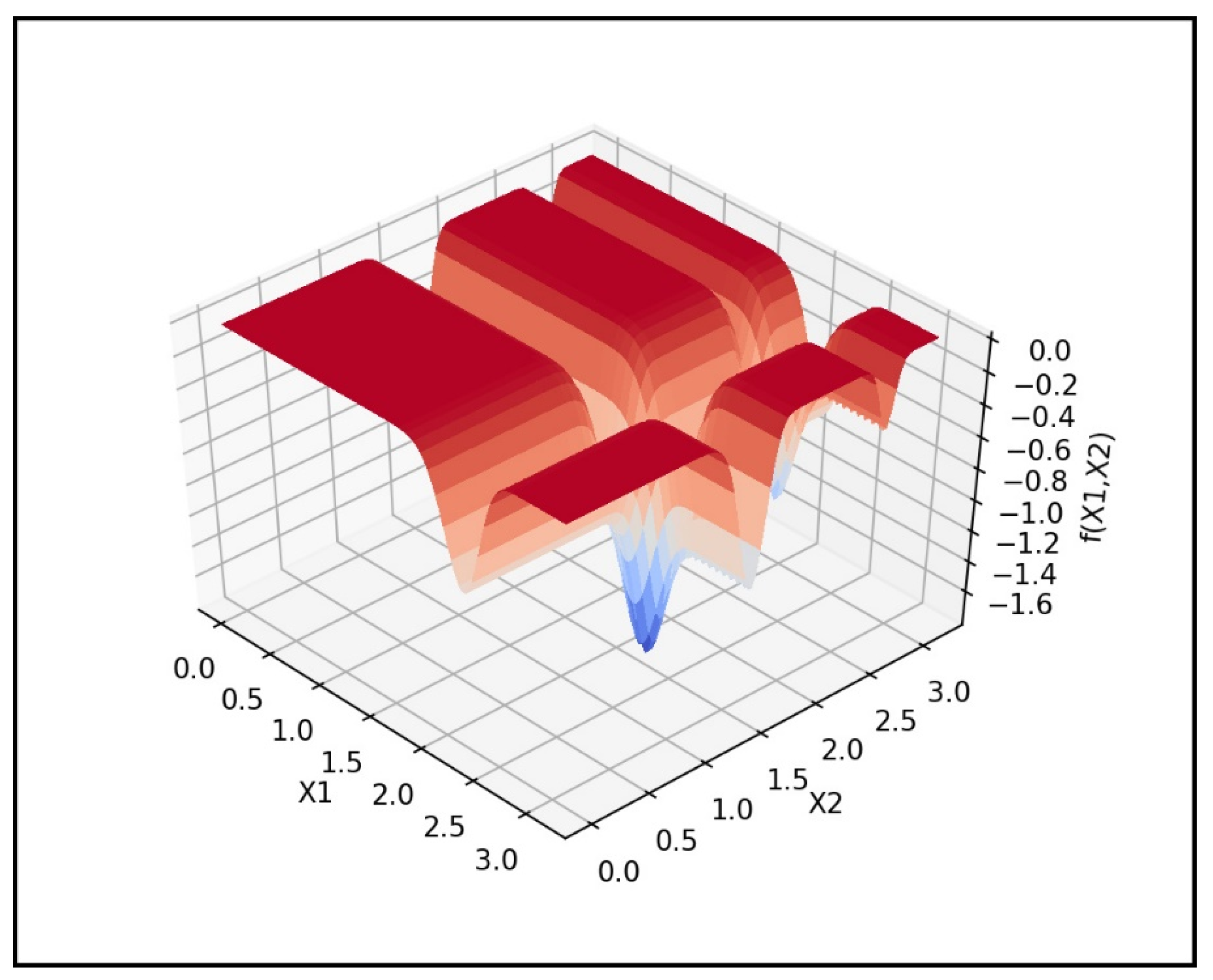
F10	Michalewicz (m = 10)	5	−4.687658	MM, S	(0, 3.14)
F11	Rosenbrock	10	0	UM, NS	(−30, 30)
F12	Rotated Hyper Ellipsoid	10	0	UM, NS	(−65.536, 65.536)
F13	Zakharov	10	0	UM, NS	(−5, 10)
F14	Rastrigin	20	0	MM, S	(−5.12, 5.12)

lists the 14 benchmark functions we have carefully curated and their associated properties. All the chosen functions are continuous and differentiable except F14 (which is discontinuous and non-differentiable). Since SPGD uses numerical differentiation, it can also handle non-differentiable functions [1]. The 14 benchmark functions were taken from [46,47].

Multi-modal functions (MM) with many local minima, non-separable (NS), and high-dimensional functions are well known to be challenging to optimize. Functions with profound flatness do not disseminate helpful information to direct the search process and are difficult to optimize (e.g., F5), especially for gradient-based algorithms [46]. According to [46], the following are certain classes of function, which are difficult to optimize:

• Functions in which the global minima is very close to the local minima (F6).
• Functions with a narrowed curved valley (F2, F8, F11).
• Functions in which the area that contains the global optimum is small with respect to the whole function space (F10).
• Functions with a significant magnitude difference between their hypersurface and domain (F4).

Further, in [47] there is a compiled list of classical benchmark functions that classify the functions into six categories (based on geometry), namely [47]: many local minima (F1,F3,F9,F14,F6), bowl-shaped (F12), valley-shaped (F11), steep-ridges (F10), plate-shaped (F5, F13), and others (F2, F8). Our assorted test suite includes at least one function from the various types mentioned above, thus ensuring diversity.

The proposed SPGD algorithm has four primary hyperparameters, namely, the number of GD instances/threads (N), number of episodes (Ep), number of iterations/GD steps per episodes (Nip), and number of stable episodes (NSEp). We test the SPGD on the benchmark functions for different combinations of these hyperparameters. This experiment aims to see how these hyperparameter choices influence SPGD.

Table 3. Various hyperparameter combinations of SPGD.

Name of The Hyperparameter Combination	Number of GD Instances (N)	Number of Episodes (Ep)	Number of Iterations per Episodes (Nip)	Number of Stable Episodes (NSEp)	Number of Iterations at Worst Case (IF Ep(Converge) = N)
C1	100	50	20	10	100,000
C2	50	50	20	10	50,000
C3	25	50	30	10	37,500
C4	25	50	20	10	25,000
C5	25	50	25	5	25,000

lists the various combinations we have chosen to test. C1 is the most computationally costly combination out of all. In the worst case (if SPGD does not converge), C1 can take 100,000 iterations. We halve the number of individuals in C2. For the remaining combinations, we set the n = 25 to see how SPGD performs with fewer individuals. In C3, we increase Nip to 30, while in C5, we reduce NSEp to five to study the corresponding effect on performance and convergence.

To test the sensitivity of the aforementioned hyperparameters for each benchmark function, we perform 50 independent runs with different initial random seeds. All experiments (in this and the upcoming sections) are performed in python 3 (Jupyter Notebook) over the Asus TUF–FX504 laptop computer with Intel i5-8300H CPU @ 2.30 GHz and 8 GB RAM, running Windows 10 operating system. The python implementations of the functions in Table 2 are taken from [48].

The best, worst, mean, standard deviation (SD), and success rate (SR) are popular metrics to evaluate an OP algorithm’s performance on the benchmark functions. According to [7], best, mean, and SD are used to evaluate the accuracy and efficiency of the OP algorithm. In contrast, SR and worst are used to evaluate the convergence speed and robustness of the algorithm. A lower SD also indicates robustness [49]. SR is defined as the ratio of successful runs out of the 50 runs [7]. A single run of an OP algorithm is deemed successful if it manages to find the global optimum within an acceptable error margin. The error measure is adopted from [8], which is “(f(x) − f(x*)), where x is the best solution obtained by algorithms in one run and x* is the well-known global optimum of each benchmark function” [8]. If (f(x) − f(x*)) < 10⁻⁶ for a run, then it is declared as a successful run. The average number of episodes taken to converge (Mean_ Ep_(Converge)) is tabulated to observe the convergence performance of SPGD. With these evaluation criteria, we benchmark the test functions with SPGD for various combinations of its hyperparameters.

Table 4. Results of numerical experiments performed on the selected benchmark functions for various hyperparameter combinations of SPGD.

Function Id	Hyper Parameter Combination	Best	Worst	Mean	SD	SR	Mean_Ep(Converge)
F1 (Ackley)	C1	0	0	0	0	1	16
	C2	0	0	0	0	1	15.9
	C3	0	0	0	0	1	16
	C4	0	0	0	0	1	16.46
	C5	0	0	0	0	1	10.92
F2 (Beale)	C1	0	7.57467 × 10−5	1.51734 × 10−6	1.07118 × 10−5	0.98	36.16
	C2	0	6.0145 × 10−4	2.38475 × 10−5	1.0895 × 10−4	0.94	45.6
	C3	0	1.05487 × 10−5	0	2.41421 × 10−6	0.92	45.76
	C4	0	2.20053 × 10−3	7.19695 × 10−5	3.4012 × 10−4	0.86	47.4
	C5	0	5.29452 × 10−3	1.29834 × 10−3	1.58691 × 10−3	0.34	22.18
F3 (EggHolder)	C1	−959.640662	−935.337951	−956.512989	7.4296201	0.0	25.76
	C2	−959.640662	−894.578898	−945.252029	21.331546	0.0	33.86
	C3	−959.640588	−786.525994	−931.834921	32.667300	0.0	30.16
	C4	−959.639814	−786.525994	−927.660588	34.371745	0.0	30
	C5	−959.636808	−786.525994	−925.475682	38.169414	0.0	13.58
F4 (Gold-Stein Price)	C1	3.0	3.0	3.0	0	1	11
	C2	3.0	3.0	3.0	0	1	34.22
	C3	3.0	3.0	3.0	0	1	11.16
	C4	3.0	3.0	3.0	0	1	11.14
	C5	3.0	3.0	3.0	0	1	6
F5 (Matyas)	C1	0	0	0	0	1	16.57
	C2	0	0	0	0	1	22.02
	C3	0	0	0	0	1	26.78
	C4	0	0	0	0	1	23.1
	C5	0	0	0	0	1	17.48
F6 (Schaffer)	C1	0.29257863	0.29257863	0.29257863	0	1	22.42
	C2	0.29257863	0.29257863	0.29257863	0	1	25.58
	C3	0.29257863	0.29257863	0.29257863	0	1	28.12
	C4	0.29257863	0.29257876	0.29257863	0	1	30.12
	C5	0.29257863	0.29261529	0.29257941	5.18320 × 10−6	0.96	21.96
F7 (Tripod)	C1	0	0.02197657	0.00091925	0.00322785	0.18	37.6
	C2	0	0.11337406	0.00637666	0.01931453	0.14	37.02
	C3	0	0.12792996	0.00730648	0.02230414	0.1	35.34
	C4	0	0.08701752	0.00514379	0.01680644	0.04	36.62
	C5	2.25691 × 10−5	0.22906872	0.03468707	0.05019722	0	18.74
F8 (Colville)	C1	0	0	0	0	1	16.22
	C2	0	0	0	0	1	16.92
	C3	0	0	0	0	1	16.78
	C4	0	0	0	0	1	17.38
	C5	0	1.58140399	0.03205936	0.22360284	0.96	12.56
F9 (Griewank)	C1	0	0.00986467	0.00034521	0.00172647	0.96	40.65
	C2	0	0.16277361	0.01084491	0.03119835	0.8	44.76
	C3	0	0.39174897	0.01843029	0.06740692	0.72	43.61
	C4	0	0.12318531	0.00808213	0.02397737	0.74	47.1
	C5	0	5.82227555	0.15844181	0.86088410	0.7	39.86
F10 (Michaelwicz)	C1	−4.687658	−3.52489854	−4.48758298	0.29075257	0.26	44.86
	C2	−4.687658	−3.52498727	−4.38087234	0.3646653	0.18	46.28
	C3	−4.6876581	−3.4938926	−4.32720985	0.3697356	0.18	45.9
	C4	−4.6876581	−3.22626745	−4.2453005	0.3777910	0.1	47.44
	C5	−4.6868078	−2.13186393	−3.08535244	0.64314420	0	16.78
F11 (Rosenbrock)	C1	0	9.97379 × 10−5	1.99475 × 10−6	1.41050 × 10−5	0.98	41.56
	C2	0	7.92577600	0.15851552	1.1208739	0.98	29.5
	C3	0	0.02173848	0.00043476	0.00307428	0.98	39.14
	C4	0	2.33355643	0.05058394	0.33060934	0.96	42.98
	C5	0	99824.3438	2544.21169	14557.6125	0.66	32.06
F12 (Rotated Hyper Ellipsoid)	C1	0	0	0	0	1	22.22
	C2	0	0	0	0	1	23.98
	C3	0	0	0	0	1	21.26
	C4	0	0	0	0	1	24.12
	C5	0	1.85962 × 10−5	0	2.62984 × 10−7	0.96	16.3
F13 (Zakharov)	C1	0	0	0	0	1	44.96
	C2	0	0	0	0	1	48.46
	C3	0	0	0	0	1	46.84
	C4	0	0	0	0	1	49.04
	C5	0	58.1560150	6.75172438	15.3146739	0.54	30.42
F14 (Rastrigin)	C1	0	0	0	0	1	12
	C2	0	0	0	0	1	12.34
	C3	0	0	0	0	1	11.76
	C4	0	0	0	0	1	13.4
	C5	0	0	0	0	1	8.44

shows the results of SPGD in terms of the discussed evaluation metrics. Values below 10⁻⁶ are shown as 0.

To quote [50], “Derivative based learning techniques do not fare well for finding global optimal solutions of the nonlinear problems having many local optimal solutions,” despite this, SPGD performs decently well. For functions F1, F4, F5, F6, F8, and F11-F14, SPGD consistently gives an SR close to 1 (or at least greater than 0.9), SD < 1, and mean closer to the optimum for almost all (except C5) of the hyperparameter combinations. An SR greater than 0.9 indicates that, nine times, out of 10 runs, SPGD will most likely find the exact optimum. For functions F2, F3, F7, and F9, SPGD gives a competitive performance compared to other OP algorithms (see Section 3.2). This indicates that SPGD, in general, is accurate, efficient, robust, and has good convergence capability.

Let us inspect other test functions for which SPGD does not give perfect optimal performance. F11, a difficult function to optimize [47,50,51], despite having a good SR (⪆0.9), has a very high worst value for all hyperparameter combinations. This is because of its narrow parabolic-shaped flat valley [52], which misdirects the SPGD to converge in a suboptimal minimum in a few of the runs. This results in a high worst value which correspondingly increases its mean value and SD. Note that increasing the number of GD steps (Nip = 30) in C3 improves the performance significantly for F11. Functions F2, F5, and F13 have profound flatness, and flatness does not disseminate directional information to guide the search [46]. F2 additionally has frequent direction changes in the function [46], with its minimum located in a narrow-curved valley [51] which causes GD to oscillate [31]. For F5 and F13, SPGD performs well; while for F2, the worst value is high for certain combinations, but still, its SR is quite satisfactory (⪆0.8).

Functions F3 and F9 are highly multi-modal, non-separable, and are even difficult to be optimized by other OP algorithms (see Section 3.2). For F9, the number of local minima increases exponentially with increasing dimensionality [53]. Despite this, the mean value and SD are closer to zero, with SR ⪆0.7 for most hyperparameter combinations.

F10 is another multi-modal function with numerous valleys and ridges, which are very difficult for SPGD to optimize. It has D! (dimension = D) local minima (in our case 5! = 120) [52]. Added to steep valleys and ridges [54], F10 also has numerous flat surfaces (see Figure 1). The combination of multi-modality with flatness and ridges makes F10 particularly difficult for GD-based algorithms to optimize.

For all unimodal functions, SPGD performs near optimally, except F2, for which SPGD slightly underperforms due to the reasons discussed earlier. Nevertheless, for F2, the mean value is very close to the optimum. This good performance with UM functions shows that SPGD is good with its exploitation capabilities. For MM functions F1, F4, and F14, SPGD performs optimally. In comparison, other MM functions, F3, F9, and F10, are quite challenging functions in general and in specific for GD-based algorithms. However, SPGD yields competitive performance for these functions (see Section 3.2). Hence, SPGD balances exploration and exploitation effectively.

Regarding the hyperparameter combinations (from Table 3), it can be observed that SPGD performs the best for the C1 combination, which is quite expected since C1 is the most computationally costly combination. Halving the population to 50 very slightly reduces the performance for F2, F3, F7, F9, and F10 alone. For the remaining combination, the population is set to 25 to keep the computational cost minimal.

Between C3, C4, and C5, the difference is, in C3, Nip is set to 30, while in C5, NSEp is decreased to 5 to solicit the corresponding effects. Increasing the number of GD steps boosts SR and other metrics for F2, F3, F10, and F11. Interestingly for F9, C3 performs marginally inferior compared to C4; this might be due to the oscillatory nature of GD [31]. It should be noted that increasing the GD steps almost always results in a better performance but not necessarily. C5 drastically reduces the number of episodes taken to converge for all 14 benchmark functions at the cost of performance degradation. For several functions (F2, F8, F9, F11, F13), the degradation is quite significant, and this is due to pre converging in fewer episodes on suboptimal values.

The episode at which SPGD (for combination C4) converges for each of the independent 50 runs is plotted as a box plot in Figure 2 for each test function. The Ep_Converge deviates significantly for most of the functions except F1, F4, F8, F9, and F14. A small NSEp should be preferred when the problem is to be optimized quickly or in situations where a suboptimal solution is adequate.

With this experiment, we conclude that the combination C4 strikes a good balance between reasonable performance and computational cost. C4 is the most computationally economical combination yet yields a practically satisfactory performance (low SD, high SR, mean closer to optimum) for most of the benchmark functions (F1, F2, F4-F6, F8, F11-F14). We fix this combination of hyperparameters as the default choice for the SPGD algorithm. The experiments performed in the subsequent sections use this default combination. In the next subsection, we compare SPGD with other popular OP algorithms.

3.2. Comparison

It is requisite to study how the proposed algorithm performs compared to other established, commonly used OP algorithms. We choose to compare the proposed SPGD algorithm with the global optimization algorithms in the scipy.optimize package [55] of the widely used [56] opensource “SciPy” library. SciPy is the state-of-the-art, high-level, continuously developed python library for performing scientific and numeric computation [57]. SciPy is known for its user-friendly [58] interfaces, which in turn serve as a great quick start to solve applied mathematical and engineering problems even for “non-professional programmers” [57].

For global optimization, the scipy.optimize package provides the implementation of five assorted OP algorithms. The five algorithms, along with their default values for hyperparameters, can be found in

Table 5. Hyperparameters for the five global optimization algorithms from the SciPy library additionally with PSO.

S.NO	Algorithm	Hyperparameters with Default Values
1	Basinhopping (BH) [59]	func, x0, niter = 100, T = 1.0, stepsize = 0.5, minimizer_kwargs = None, take_step = None, accept_test = None, callback = None, interval = 50, disp = False, niter_success = None, seed = None
2	Simplicial Homology Global Optimization (SHGO) [60]	func, bounds, args = (), constraints = None, n = None, iters = 1, callback = None, minimizer_kwargs = ’SLSQP’, options = None, sampling_method = ‘simplicial’
3	Dual Annealing (DAE) [61]	func, bounds, args = (), maxiter = 1000, local_search_options = {}, initial_temp = 5230.0, restart_temp_ratio = 2 × 10−5, visit = 2.62, accept = −5.0, maxfun = 10,000,000.0, seed = None, no_local_search = False, callback = None, x0 = None
4	Differential Evolution (DE) [62]	func, bounds, args = (), strategy = ‘best1bin’, maxiter = 1000, popsize = 15, tol = 0.01, mutation = (0.5, 1), recombination = 0.7, seed = None, callback = None, disp = False, polish = True, init = ‘latinhypercube’, atol = 0, updating = ‘immediate’, workers = 1, constraints = (), x0 = None
5	Brute [63]	func, ranges, args = (), Ns = 20, full_output = 0, finish = <function fmin>, disp = False, workers = 1
6	Particle Swarm Optimization (PSO) [64,65]	fun, x0, confunc = None, friction = 0.8, max_velocity = 5., g_rate = 0.8,l_rate = 0.5, max_iter = 1000, stable_iter = 100, ptol = 1 × 10−6, ctol = 1 × 10−6, callback = None

. We have additionally included the PSO algorithm whose implementation closely mimics the scipy.optimize interface. It can be seen from Table 5 that most of these algorithms have quite a lot of hyperparameters, significantly more than our proposed SPGD algorithm. The details of the hyperparameters can be seen in the corresponding references [59,60,61,62,63,64]. SHGO is a deterministic algorithm [65]. Note that basinhopping and PSO do not have the ‘bounds’ parameter. The corresponding implication is that they might go out of the prescribed bounds (LB, UB) for some test problems. For Both these algorithms we need to specify a D-dimensional starting point. Uniform distribution is used to randomly generate a starting point (within the prescribed bounds) for each of the 50 independent runs (with random seeds). For PSO, the number of particles is set to 100, and thus 100 random starting points are generated, whereas, for basinhopping, a single point is generated.

We have decided to compare SPGD to these algorithms with their default values of hyperparameters. This is mainly done for two reasons. Firstly, the algorithms chosen to be compared are very diverse, ranging from brute force to evolutionary (DE), annealing (DAE)-based, algebraic topology (SHGO)-based, particle-based, and gradient-free algorithms. This diversity implies that some algorithms might need more resources for some problems (population, iterations, etc.) to perform optimally, while others might differ with specific nuances to cater for. Secondly, since SciPy is meant to be a high-level quick-to-use library, scientists will tend to use it as a black-box optimizer for quick experimentation without getting lost in the intricacy of the underlying OP algorithms [57]. As a consequence, no efforts to change the default hyperparameters might be made. So, it makes sense to ”practically” compare these algorithms in their most likely to be used default configurations.

Table 6. Comparative results of SPGD-C4 with state-of-the-art algorithms from the global optimization suite of the SciPy library.

Function Id	Algorithm	Best	Worst	Mean	SD	SR
F1 (Ackley)	BH	0	1.36472421	0.13514784	0.25274851	0.68
	SHGO	0	0	0	0	1
	Dual_Ann	0	0	0	0	1
	DiffEvoul	0	0.2801272	0.0056025	0.0396159	0.98
	Brute	0.78352294	0.78352294	0.78352294	0	0
	PSO	0	0	0	0	1
	SPGD	0	0	0	0	1
F2 (Beale)	BH	0	0	0	0	1
	SHGO	0	0	0	0	1
	Dual_Ann	0	0	0	0	1
	DiffEvoul	0	0.7336411	0.0146728	0.1037525	0.98
	Brute	0	0	0	0	1
	PSO	0	0	0	0	1
	SPGD	0	0.00220053	7.196953 × 10−5	0.00034012	0.86
F3 (EggHolder)	BH #	−1102.97164	−88.3042594	−546.101393	222.441807	0
	SHGO	−935.337951	−935.337951	−935.337951	0	0
	Dual_Ann	−959.640662	−888.949125	−931.473470	29.64637	0
	DiffEvoul	−959.640662	−786.52599	−910.403744	49.9705672	0
	Brute #	−976.911000	−976.911000	−976.911000	0	0
	PSO #	−976.911000	−716.67150	−893.762654	69.4243212	0
	SPGD	−959.639814	−786.525994	−927.660588	34.3717458	0
F4 (Gold-Stein Price)	BH	3.0	3.0	3.0	0	1
	SHGO	3.0	3.0	3.0	0	1
	Dual_Ann	3.0	3.0	3.0	0	1
	DiffEvoul	3.0	3.0	3.0	0	1
	Brute	3.0	3.0	3.0	0	1
	PSO	3.0	3.0	3.0	0	1
	SPGD	3.0	3.0	3.0	0	1
F5 (Matyas)	BH	0	0	0	0	1
	SHGO	0	0	0	0	1
	Dual_Ann	0	0	0	0	1
	DiffEvoul	0	0	0	0	1
	Brute	0	0	0	0	1
	PSO	0	0	0	0	1
	SPGD	0	0	0	0	1
F6 (Schaffer)	BH	0.29257863	0.49741695	0.42685063	0.07275457	0.14
	SHGO	0.50113378	0.50113378	0.50113378	0	0
	DualAnn	0.29257863	0.29387375	0.29260453	0.00018315	0.98
	DiffEvoul	0.29257863	0.29258103	0.29257869	0	0.98
	Brute	0.36131449	0.36131449	0.36131449	0	0
	PSO	0.29257863	0.29257863	0.29257863	0	1
	SPGD	0.29257863	0.29257876	0.29257863	0	1
F7 (Tripod)	BH	0	2.000000008	0.820000004	0.84972984	0.46
	SHGO	1.00000001	1.00000001	1.00000001	0	0
	DualAnn	0	1.000064264	0.620001309	0.49031536	0.38
	DiffEvoul	0	2.000000694	0.80000008	0.75592899	0.4
	Brute	1.00003641	1.00003641	1.00003641	0	0
	PSO	0	2.000000003	0.56000000	0.61145527	0.5
	SPGD	0	0.0870175274	0.0051437912	0.01680644	0.04
F8 (Colville)	BH	0	0	0	0	1
	SHGO	0	0	0	0	1
	Dual_Ann	0	0	0	0	1
	DiffEvoul	0	0	0	0	1
	Brute	0	0	0	0	1
	PSO	0	7.84998268	0.6040938	1.3746632	0.46
	SPGD	0	0	0	0	1
F9 (Griewank)	BH	0.24868915	132.830121	17.4293518	22.128654	0
	SHGO	0	0	0	0	1
	DualAnn	0	0.066493	0.0220203	0.0154676	0.1
	DiffEvoul	0	0.05662099	0.0136467	0.0106129	0.14
	Brute	1.19740690	1.19740690	1.19740690	0	0
	PSO	0.00985728	0.30542824	0.08472009	0.0560294	0
	SPGD	0	0.12318531	0.00808213	0.02397737	0.74
F10 (Michaelwicz)	BH #	−4.74614390	−3.33129293	−4.38273363	0.3484707	0.1
	SHGO	−3.53609746	−3.53609746	−3.53609746	0	0
	DualAnn	−4.68765817	−4.68765817	−4.68765817	0	1
	DiffEvoul	−4.68765817	−4.3748963	−4.6408507	0.0651459	0.38
	Brute	−4.6876580	−4.6876580	−4.6876580	0	1
	PSO	−4.64589536	−2.6401023	−3.8328507	0.5415107	0
	SPGD	−4.6876581	−3.22626745	−4.2453005	0.3777910	0.1
F11 (Rosenbrock)	BH	0	0	0	0	1
	SHGO	0	0	0	0	1
	DualAnn	0	0	0	0	1
	DiffEvoul	0	3.98658234	0.55812114	1.3973353	0.86
	Brute	Memory Error
	PSO	0.62903529	458.440177	53.6217016	93.8592738	0
	SPGD	0	2.33355643	0.05058394	0.33060934	0.96
F12 (Rotated Hyper Ellipsoid)	BH	0	0	0	0	1
	SHGO	0	0	0	0	1
	DualAnn	0	0	0	0	1
	DiffEvoul	0	0	0	0	1
	Brute	Memory Error
	PSO	0	0.03187133	0.00107759	0.005112	0.76
	SPGD	0	0	0	0	1
F13 (Zakharov)	BH	0	0	0	0	1
	SHGO	20.5109595	20.5109595	20.5109595	0	0
	DualAnn	0	0	0	0	1
	DiffEvoul	0	0	0	0	1
	Brute	Memory Error
	PSO	0	1.26451010	0.09737653	0.21157360	0.02
	SPGD	0	0	0	0	1
F14 (Rastrigin)	BH	4.97479528	26.8638491	11.541520	4.2641043	0
	SHGO *	Maximum Time Limit Exceeded
	DualAnn	0	0	0	0	1
	DiffEvoul	8.95463151	46.7629849	21.2125049	7.7342163	0.0
	Brute	Memory Error
	PSO	28.4366707	98.5430492	55.253022	15.376534	0
	SPGD	0	0	0	0	1

^# The minima location found is out of bounds. We ignore these results. * After 6 h of processing time, no output is printed even for a single run, and hence terminated.

shows the results of SPGD (C4) and the other six OP algorithms for the 14 test functions in terms of metrics discussed in the previous subsection. Values below 10⁻⁶ are shown as zero.

It is not easy to distill one single algorithm as successful out of all others from Table 6. Let us take one crucial evaluation metric, SR, to majorly gauge the performance to make things simple. As the name suggests, SR measures how often the algorithm is successful/finds the optimum. As mentioned in the previous section, an SR greater than 0.9 strongly indicates the practical applicability of an OP algorithm. We make another table,

Table 7. The list of test functions for which each algorithm yields an SR greater than 0.9.

Algorithms	Functions	Number of Functions
BH	F2, F4, F5, F8, F11, F12, F13	7
SHGO	F1, F2, F4, F5, F8, F9, F11, F12	8
DAE	F1, F2, F4, F5, F6, F8, F10, F11, F12, F13, F14	11
DE	F1, F2, F4, F5, F6, F8, F12, F13	8
Brute	F2, F4, F5, F6, F8, F10	6
PSO	F1, F2, F4, F5, F6	5
SPGD	F1, F4, F5, F6, F8, F11, F12, F13, F14	9

, which lists the number of functions for which each algorithm yields a success rate greater than 0.9.

From Table 7, it can be observed that DAE performs the best out of all others in its default configuration. SPGD performs the second best. DE and SHGO are successful for eight test functions. SHGO is known to work well with low-dimensional problems and not so well with high-dimensional functions [60,65]. For F14 (20-dimensional), after 6 h of execution SHGO, it does not return any results for even a single run. Similarly, Brute also performs well for low-dimensional functions, and for high-dimensional functions (>10-dimensional), Brute does not execute due to memory error. Since PSO and BH do not have the ”bounds” parameter, they go out of bounds for some functions (F3 and F10).

Functions F3, F7, and F9 (except for SHGO) did not make it into Table 7. This shows how complex these three functions are. F3 and F9 have a large parametric solution space. Further, for F3, the global optimum lies at the extreme corner [66]. On closer observation, it can be seen that SPGD indeed performs well for these two functions. For F3, DAE again performs better in mean and SD, and SPGD closely follows as the second best. For F9, SHGO performs the best with an SR of perfect 1. In comparison, SPGD gives an SR of 0.74, which is way higher than all other algorithms.

F7 is non-differentiable, is discontinuous, has a sizeable parametric search space, and has two local minima at ($x_1$ = −50, $x_2$ = 50) and ($x_1$ = 50, $x_2$ = 50) with corresponding function values as 1 and 2 [67]. The global minimum is located at ($x_1$ = 0, $x_2$ = −50). SR of SPGD for F7 is very low compared to other algorithms, but SPGD outperforms all other algorithms in worst, mean, and SD. If we look at the worst value of F7 for all other algorithms, it is either 1 or 2, implying that those algorithms have been trapped in one of the two local optima. The worst value of SPGD for F7 is 0.0870175274 (occurs at $x_1$ = 0.08701752, $x_2$ = −50, which is very close to the global minima location). This shows that SPGD does not get caught in the local minima even in a single run. Though SPGD locates the valley containing the global minima in every single run, it fails to pinpoint the exact location of the global minima (since the gradient information obtained through numerical differentiation is unreliable as the function is non-differentiable and discontinuous); this is the reason behind the low SR. Nevertheless, F7 supports the claim that SPGD has a highly competitive capacity to escape local optimums, thus exhibiting a good balance between exploration and exploitation.

To summarize, considering the positive performance for the functions F3, F7, and F9, SPGD gives a competitive performance to other OP algorithms of the SciPy suite. It is acknowledged that if the hyperparameters of these SciPy algorithms are tuned appropriately, they might yield much better performance and can outperform SPGD. Nevertheless, as discussed, we venture for a ”practical comparison”, in which SPGD indeed fares well.

3.3. Discussion

The extensive numerical experiments performed in this section show that the proposed algorithm is robust enough to solve various OP problems. In the comparison with SciPy’s advanced OP algorithms, SPGD is only bested by DAE. DAE outperforms SPGD for F2 and F10 in terms of SR. For F2, SPGD yields an SR of 0.86, which is relatively high, whereas F10, as discussed earlier, is fundamentally difficult for gradient-based algorithms. However, upon closer observation, it can be seen that even SPGD outperforms DAE for some functions like F9 and F7 (except SR) in terms of all the metrics. This indicates that DAE does not entirely overshadow SPGD, and it is a close call between SPGD and DAE. We re-emphasize that our motivation is to develop a quick-start, easy-to-understand OP algorithm that is competent enough to be used in practice. We believe that SPGD indeed caters to this.

The algorithm proposed in this paper runs multiple parallel instances of vanilla gradient descent guided by the “DCA” paradigm and inspired by the human search party metaphor. Simple vanilla GD obtains practical efficacy when run under the paradigm of DCA. Further, owing to the simplicity of the constant learning rate GD and the relatable human search party metaphor, we believe the proposed SPGD algorithm is arguably simple but robust enough to be used in solving OP problems.

4. Conclusions

A sheer number of global OP algorithms have been published in the literature. Most of them strive to give the best performance possible. Amidst this, our goal was to propose an OP algorithm that is simple (few straightforward hyperparameters), familiar, and easier to comprehend while satisfactory enough to be used in practice. Effectively, this would be an OP algorithm that can be used as a quick-start solution, but with the knowledge of what is happening under the hood. Constant learning rate GD is one of the preliminary OP algorithms, which is easier to understand [32]. SPGD coordinates multiple GD instances running parallel to find the global optimum based on the human search party metaphor. The numerical experiments have demonstrated SPGD’s potential to solve problems, and we believe they provide enough evidence for its existence.

References

- D’Angelo, G.; Palmieri, F. GGA: A modified genetic algorithm with gradient-based local search for solving constrained optimization problems. Inf. Sci. 2021, 547, 136–162. [Google Scholar] [CrossRef]
- Zhu, C.; Byrd, R.H.; Lu, P.; Nocedal, J. Algorithm 778: L-BFGS-B: Fortran subroutines for large-scale bound-constrained optimization. ACM Trans. Math. Softw. (TOMS) 1997, 23, 550–560. [Google Scholar] [CrossRef]
- Cong, Y.; Wang, J.; Li, X. Traffic Flow Forecasting by a Least Squares Support Vector Machine with a Fruit Fly Optimization Algorithm. Procedia Eng. 2016, 137, 59–68. [Google Scholar] [CrossRef] [Green Version]
- Mashwani, W.K. Comprehensive survey of the hybrid evolutionary algorithms. Int. J. Appl. Evol. Comput. (IJAEC) 2013, 4, 1–19. [Google Scholar] [CrossRef] [Green Version]
- Ferreiro, A.M.; García-Rodríguez, J.A.; Vázquez, C.; e Silva, E.C.; Correia, A. Parallel two-phase methods for global optimization on GPU. Math. Comput. Simul. 2019, 156, 67–90. [Google Scholar] [CrossRef]
- Sutton, R.S.; Barto, A.G. Reinforcement Learning: An Introduction; MIT Press: Cambridge, MA, USA, 2018. [Google Scholar]
- Wu, H.S.; Zhang, F.M. Wolf pack algorithm for unconstrained global optimization. Math. Probl. Eng. 2014, 2014, 465082. [Google Scholar] [CrossRef] [Green Version]
- Mohamed, A.W.; Hadi, A.A.; Mohamed, A.K. Gaining-sharing knowledge based algorithm for solving optimization problems: A novel nature-inspired algorithm. Int. J. Mach. Learn. Cybern. 2020, 11, 1501–1529. [Google Scholar] [CrossRef]
- Dorigo, M.; Maniezzo, V.; Colorni, A. Ant system: Optimization by a colony of cooperating agents. IEEE Trans. Syst. Man Cybern. Part B (Cybernetics) 1996, 26, 29–41. [Google Scholar] [CrossRef] [Green Version]
- Pourpanah, F.; Wang, R.; Lim, C.P.; Yazdani, D. A review of the family of artificial fish swarm algorithms: Recent advances and applications. arXiv 2020, arXiv:2011.05700. Available online: https://arxiv.org/abs/2011.05700 (accessed on 10 February 2022).
- Mirjalili, S. Moth-flame optimization algorithm: A novel nature-inspired heuristic paradigm. Knowl. Based Syst. 2015, 89, 228–249. [Google Scholar] [CrossRef]
- Zhao, R.Q.; Tang, W.S. Monkey algorithm for global numerical optimization. J. Uncertain Syst. 2008, 2, 165–176. [Google Scholar]
- Mirjalili, S.; Mirjalili, S.M.; Lewis, A. Grey wolf optimizer. Adv. Eng. Softw. 2014, 69, 46–61. [Google Scholar] [CrossRef] [Green Version]
- Yang, X.-S. A New Metaheuristic Bat-Inspired Algorithm. In Nature Inspired Cooperative Strategies for Optimization (NICSO 2010); Springer: Berlin/Heidelberg, Germany, 2010; pp. 65–74. [Google Scholar]
- Das, S.; Biswas, A.; Dasgupta, S.; Abraham, A. Bacterial Foraging Optimization Algorithm: Theoretical Foundations, Analysis, and Applications. Auton. Robot. Agents 2009, 3, 23–55. [Google Scholar]
- Mirjalili, S.; Lewis, A. The whale optimization algorithm. Adv. Eng. Softw. 2016, 95, 51–67. [Google Scholar] [CrossRef]
- Karaboga, D.; Akay, B. A comparative study of Artificial Bee Colony algorithm. Appl. Math. Comput. 2009, 214, 108–132. [Google Scholar] [CrossRef]
- Gandomi, A.H.; Alavi, A.H. Krill herd: A new bio-inspired optimization algorithm. Commun. Nonlinear Sci. Numer. Simul. 2012, 17, 4831–4845. [Google Scholar] [CrossRef]
- Rao, R. Review of applications of TLBO algorithm and a tutorial for beginners to solve the unconstrained and constrained optimization problems. Decis. Sci. Lett. 2016, 5, 1–30. [Google Scholar]
- Kashan, A.H. League Championship Algorithm (LCA): An algorithm for global optimization inspired by sport championships. Appl. Soft Comput. 2014, 16, 171–200. [Google Scholar] [CrossRef]
- Eskandar, H.; Sadollah, A.; Bahreininejad, A.; Hamdi, M. Water cycle algorithm—A novel metaheuristic optimization method for solving constrained engineering optimization problems. Comput. Struct. 2012, 110, 151–166. [Google Scholar] [CrossRef]
- Cuevas, E.; Cienfuegos, M.; Zaldivar-Navarro, D.; Perez-Cisneros, M.A. A swarm optimization algorithm inspired in the behavior of the social-spider. Expert Syst. Appl. 2013, 40, 6374–6384. [Google Scholar] [CrossRef] [Green Version]
- Yang, X.S.; Deb, S. Cuckoo search via Lévy flights. In Proceedings of the 2009 World Congress on Nature & Biologically Inspired Computing (NaBIC), Coimbatore, India, 9–11 December 2009. [Google Scholar]
- Moghdani, R.; Salimifard, K. Volleyball premier league algorithm. Appl. Soft Comput. 2018, 64, 161–185. [Google Scholar] [CrossRef]
- Rand, D.; Greene, J.D.; Nowak, M.A. Spontaneous giving and calculated greed. Nature 2012, 489, 427–430. [Google Scholar] [CrossRef] [PubMed]
- Grossack, M.M. Some effects of cooperation and competition upon small group behavior. J. Abnorm. Soc. Psychol. 1954, 49, 341. [Google Scholar] [CrossRef]
- Forsyth, D.R. Group Dynamics; Cengage Learning: Boston, MA, USA, 2018. [Google Scholar]
- Schwartz, S.H. Individualism-collectivism: Critique and proposed refinements. J. Cross-Cult. Psychol. 1990, 21, 139–157. [Google Scholar] [CrossRef]
- Khalil, A.M.; Fateen, S.-E.K.; Bonilla-Petriciolet, A. MAKHA—A New Hybrid Swarm Intelligence Global Optimization Algorithm. Algorithms 2015, 8, 336–365. [Google Scholar] [CrossRef] [Green Version]
- Ruder, S. An overview of gradient descent optimization algorithms. arXiv 2016, arXiv:1609.04747. Available online: https://arxiv.org/abs/1609.04747 (accessed on 10 February 2022).
- Watt, J.; Borhani, R.; Katsaggelos, A.K. Machine Learning Refined: Foundations, Algorithms, and Applications; Cambridge University Press: Cambridge, UK, 2020; Chapters 3, 3.5, 3.6. [Google Scholar]
- Wang, X. Method of steepest descent and its applications. IEEE Microw. Wirel. Compon. Lett. 2008, 12, 24–26. [Google Scholar]
- Wu, X.; Ward, R.; Bottou, L. Wngrad: Learn the learning rate in gradient descent. arXiv 2018, arXiv:1803.02865. Available online: https://arxiv.org/pdf/1803.02865.pdf (accessed on 10 February 2022).
- Search Party Definition and Meaning. Available online: https://www.dictionary.com/browse/search-party (accessed on 4 January 2022).
- Dion, K.L. Group cohesion: From “field of forces” to multidimensional construct. Group Dyn. Theory Res. Pract. 2000, 4, 7. [Google Scholar] [CrossRef]
- Cormen, T.H.; Leiserson, C.E.; Rivest, R.L.; Stein, C. Introduction to Algorithms; MIT Press: Cambridge, MA, USA, 2009. [Google Scholar]
- Cohen, J.D.; McClure, S.M.; Yu, A.J. Should I stay or should I go? How the human brain manages the trade-off between exploitation and exploration. Philos. Trans. R. Soc. B Biol. Sci. 2007, 362, 933–942. [Google Scholar] [CrossRef]
- Volchenkov, D.; Helbach, J.; Tscherepanow, M.; Kühnel, S. Treasure Hunting in Virtual Environments: Scaling Laws of Human Motions and Mathematical Models of Human Actions in Uncertainty. In Nonlinear Dynamics and Complexity; Springer International Publishing: Cham, Switzerland, 2014; pp. 213–234. [Google Scholar]
- Maroti, A. RBED: Reward Based Epsilon Decay. arXiv 2019, arXiv:1910.13701. Available online: https://arxiv.org/abs/1910.13701 (accessed on 10 February 2022).
- Numpy.Random.Triangular.—NumPy v1.21 Manual. Available online: https://numpy.org/doc/stable/reference/random/generated/numpy.random.triangular.html (accessed on 27 December 2021).
- Kotz, S.; Van Dorp, J.R. Beyond Beta: Other Continuous Families of Distributions with Bounded Support and Applications; World Scientific: Singapore, 2004; Chapter 1. [Google Scholar]
- Hesse, R. Triangle distribution: Mathematica link for Excel. Decis. Line 2000, 31, 12–14. [Google Scholar]
- Leng, J. Optimization techniques for structural design of cold-formed steel structures. In Recent Trends in Cold-Formed Steel Construction; Woodhead Publishing: Sawston, UK, 2016; pp. 129–151. [Google Scholar]
- Hong, T.P.; Wang, H.S.; Lin, W.Y.; Lee, W.Y. Evolution of appropriate crossover and mutation operators in a genetic process. Appl. Intell. 2002, 16, 7–17. [Google Scholar] [CrossRef]
- Goldberg, D.E.; Holland, J.H. Genetic Algorithms and Machine Learning. Mach. Learn. 1988, 3, 95–99. [Google Scholar] [CrossRef]
- Jamil, M.; Yang, X.-S. A literature survey of benchmark functions for global optimisation problems. Int. J. Math. Model. Numer. Optim. 2013, 4, 150–194. [Google Scholar] [CrossRef] [Green Version]
- Surjanovic, S.; Bingham, D. Virtual Library of Simulation Experiments: Test Functions and Datasets. 2013. Available online: http://www.sfu.ca/~ssurjano (accessed on 25 December 2021).
- Nathanrooy. Landscapes/Single_Objective.Py at Master Nathanrooy/Landscapes. GitHub. Available online: https://github.com/nathanrooy/landscapes/blob/master/landscapes/single_objective.py (accessed on 27 December 2021).
- Tansui, D.; Thammano, A. Hybrid nature-inspired optimization algorithm: Hydrozoan and sea turtle foraging algorithms for solving continuous optimization problems. IEEE Access 2020, 8, 65780–65800. [Google Scholar] [CrossRef]
- Abiyev, R.H.; Tunay, M. Optimization of High-Dimensional Functions through Hypercube Evaluation. Comput. Intell. Neurosci. 2015, 2015, 967320. [Google Scholar] [CrossRef] [Green Version]
- Tenne, Y.; Armfield, S.W. A memetic algorithm using a trust-region derivative-free optimization with quadratic modelling for optimization of expensive and noisy black-box functions. In Evolutionary Computation in Dynamic and Uncertain Environments; Springer: Berlin/Heidelberg, Germany, 2007; pp. 389–415. [Google Scholar]
- Molga, M.; Smutnicki, C. Test functions for optimization needs. Test Funct. Optim. Needs 2005, 101, 48. [Google Scholar]
- Cho, H.; Olivera, F.; Guikema, S.D. A derivation of the number of minima of the Griewank function. Appl. Math. Comput. 2008, 204, 694–701. [Google Scholar] [CrossRef]
- Blanchard, A.; Sapsis, T. Bayesian optimization with output-weighted optimal sampling. J. Comput. Phys. 2020, 425, 109901. [Google Scholar] [CrossRef]
- Optimization and Root Finding (Scipy.Optimize)—SciPy v1.7.1 Manual. Available online: https://docs.scipy.org/doc/scipy/reference/optimize.html (accessed on 27 December 2021).
- Pypi Stats. PyPI Download Stats—SciPy. 2021. Available online: https://pypistats.org/packages/scipy (accessed on 27 December 2021).
- Varoquaux, G.; Gouillart, E.; Vahtras, O.; Haenel, V.; Rougier, N.P.; Gommers, R.; Pedregosa, F.; Jędrzejewski-Szmek, Z.; Virtanen, P.; Combelles, C.; et al. Scipy Lecture Notes. Zenodo, 2015, ⟨10.5281/zenodo.31736⟩. ⟨hal-01206546⟩. Available online: https://hal.inria.fr/hal-01206546/file/ScipyLectures-simple.pdf (accessed on 24 January 2022).
- Nunez-Iglesias, J.; Van Der Walt, S.; Dashnow, H. Elegant SciPy: The Art of Scientific Python; O’Reilly Media, Inc.: Sebastopol, CA, USA, 2017. [Google Scholar]
- Basinhopping. Scipy.Optimize.Basinhopping—SciPy v1.7.1 Manual. Available online: https://docs.scipy.org/doc/scipy/reference/generated/scipy.optimize.basinhopping.html (accessed on 27 December 2021).
- SHGO. Scipy.Optimize.Shgo—SciPy v1.7.1 Manual. Available online: https://docs.scipy.org/doc/scipy/reference/generated/scipy.optimize.shgo.html (accessed on 27 December 2021).
- Dual_Annealing. Scipy.Optimize.Dual_Annealing—SciPy v1.7.1 Manual. Available online: https://docs.scipy.org/doc/scipy/reference/generated/scipy.optimize.dual_annealing.html (accessed on 27 December 2021).
- Differential Evolution. Scipy.Optimize.Differential_Evolution—SciPy v1.7.1 Manual. Available online: https://docs.scipy.org/doc/scipy/reference/generated/scipy.optimize.differential_evolution.html (accessed on 27 December 2021).
- Brute. Scipy.Optimize.Brute—SciPy v1.7.1 Manual. Available online: https://docs.scipy.org/doc/scipy/reference/generated/scipy.optimize.brute.html (accessed on 27 December 2021).
- PSOPy. PyPI. Available online: https://pypi.org/project/psopy/ (accessed on 24 December 2021).
- Stefan Endres (MEng, BEng (Hons) in Chemical Engineering. “Shgo”. Available online: https://stefan-endres.github.io/shgo/ (accessed on 25 December 2021).
- Aly, A.; Weikersdorfer, D.; Delaunay, C. Optimizing deep neural networks with multiple search neuroevolution. arXiv 2019, arXiv:1901.05988. Available online: https://arxiv.org/abs/1901.05988 (accessed on 10 February 2022).
- Yang, E.; Barton, N.H.; Arslan, T.; Erdogan, A.T. A novel shifting balance theory-based approach to optimization of an energy-constrained modulation scheme for wireless sensor networks. In Proceedings of the 2008 IEEE Congress on Evolutionary Computation (IEEE World Congress on Computational Intelligence), Hong Kong, China, 1–6 June 2008; pp. 2749–2756. [Google Scholar]