Unconventional GVNS for Solving the Garbage Collection Problem with Time Windows


Department of Informatics, Ionian University, 7 Tsirigoti Square, 49100 Corfu, Greece
*
Author to whom correspondence should be addressed.
Technologies 2019, 7(3), 61; https://doi.org/10.3390/technologies7030061
Submission received: 31 July 2019
/
Revised: 24 August 2019
/
Accepted: 26 August 2019
/
Published: 27 August 2019
(This article belongs to the Section Information and Communication Technologies)
Abstract
:GVNS, which stands for General Variable Neighborhood Search, is an established and commonly used metaheuristic for the expeditious solution of optimization problems that belong to the NP-hard class. This paper introduces an expansion of the standard GVNS that borrows principles from quantum computing during the shaking stage. The Traveling Salesman Problem with Time Windows (TSP-TW) is a characteristic NP-hard variation in the standard Traveling Salesman Problem. One can utilize TSP-TW as the basis of Global Positioning System (GPS) modeling and routing. The focus of this work is the study of the possible advantages that the proposed unconventional GVNS may offer to the case of garbage collector trucks GPS. We provide an in-depth presentation of our method accompanied with comprehensive experimental results. The experimental information gathered on a multitude of TSP-TW cases, which are contained in a series of tables, enable us to deduce that the novel GVNS approached introduced here can serve as an effective solution for this sort of geographical problems.
1. Introduction
Optimization problems can be classified according to the difficulty associated with the computation of the optimal solution among all the available and feasible solutions. They can be further categorized into two groups based on whether they can be formulated using variables taking values from a discrete or continuous domain. Ideally, discrete optimization is an optimization problem that has discreet variables, and in such a problem, the focus is placed on finding an object like a permutation, a graph or an integer from an infinite or finite set [1]. The problems associated with continuous variables are multimodal and constrained problems. Many real world problems deal with maximization or minimization of some quantity in order to optimize some outcome. To find the best solutions, calculus serves as the main tool for practical problems. Usually, the steps involved in solving optimization problems are: drawing of a diagram that depicts the scenario, assign symbols to the diagram, conduct an analysis of the diagram that relates to known and unknown variables, and use Calculus to find extreme values.
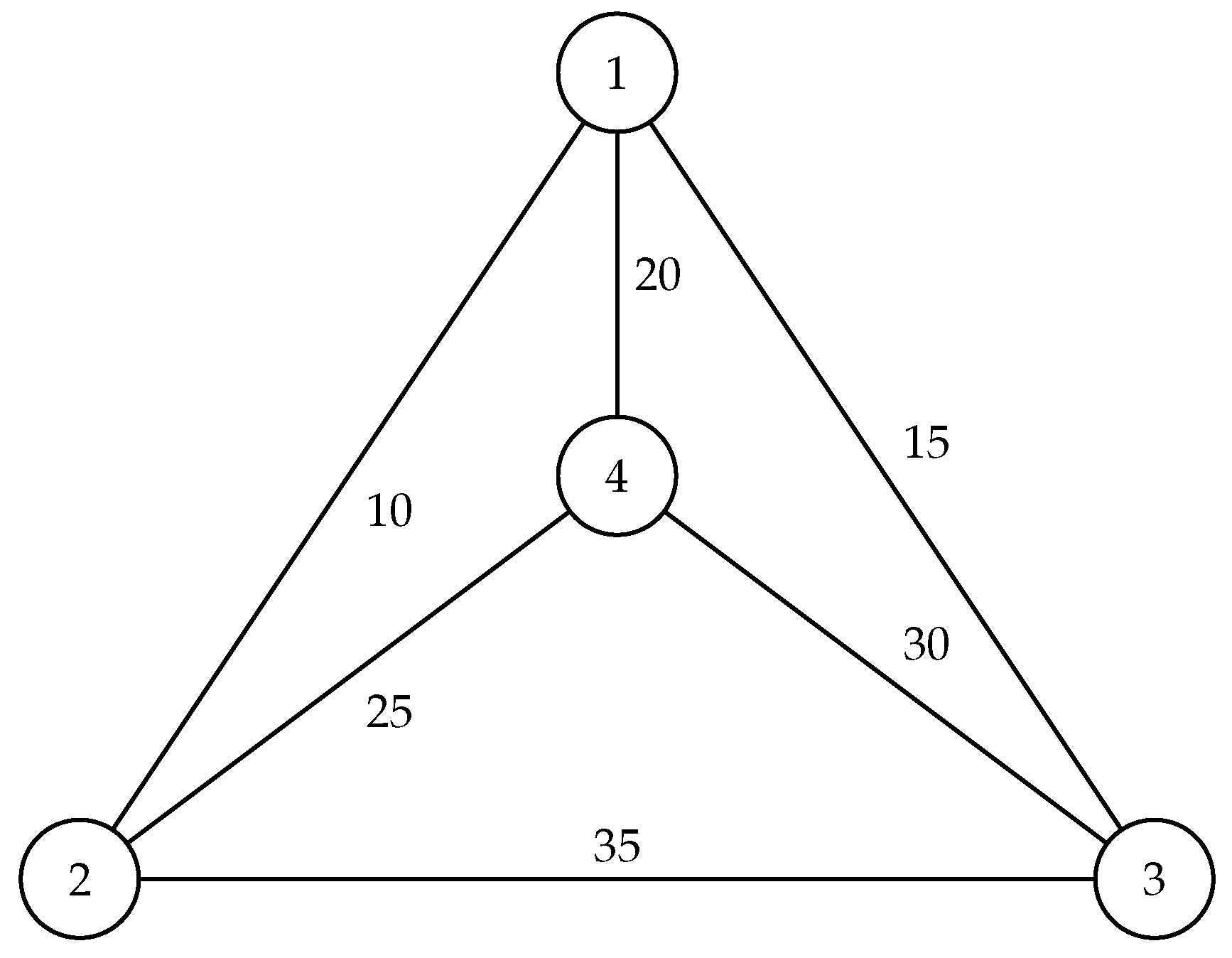
The Traveling Salesman Problem (TSP) is made up of various cities and a salesman. The salesman is obliged to visit all the cities beginning with the hometown and coming back to the same city [2]. The order in which the salesman travels is none of his concern, provided that he visits each city once and finishes at the place he began with. The cities connect each other through railway or road. The costs provide a description of the difficulty involved in traversing the edges of the underlying graph. The salesman seeks to ensure that the cost incurred in traveling remains the lowest possible. TSP is heralded as an algorithmic problem in the fields of operations research and computer science. The problem focuses on optimization whereby a better solution usually implies a faster, shorter and cheaper solution. As a mathematical problem, TSP is usually expressed in the form of a graph that describes the location of various nodes. Sir William Rowan Hamilton and Thomas Kirkman defined TSP during the 1800s, and it was first studied by Karl Menger during the 1930s at Harvard and Vienna [2]. The problem could be solved through various trials. As an algorithmic problem, its role is to find the shortest route between various locations and points that should be visited. As earlier noted, this is achieved by the salesman ensuring that the distance traveled and the travel costs remain as low as possible. Some of the applications of TSP are identification of hardware or network optimization methods. For decades, this problem has been extensively researched, and various solutions have been theorized. From the available solutions, the simplest is trying all possibilities, but it is worth noting that this is prohibitively time consuming and costly. TSP, being an NP hard problem, is not believed to possess a polynomial time solution. Practical solutions deploy heuristics that offer probability outcomes. Therefore, the produced results are often approximate rather than always optimal [2]. Instead of focusing on finding the best route, TSP usually deals with getting the cheapest solution. For example, the graph shown below Figure 1 would have a TSP tour being 1–2–4–3–1. As such, the tour’s cost would be .
The Traveling Salesman Problem with Time Windows incorporates additional constraints over the vanilla TSP; cities or clients must be visited within a specific time window. The added time constraints make the problem even more difficult. Solving the more difficult TSP-TW boils down to designing a minimum cost tour in such a way that each node is visited once at a specific time consistent with its allowable time window [3]. It should be mentioned that each node may also incorporate service time as well as travel time. The purpose of this paper is to model a real world problem as TSP with Time Windows and proceed to solve it with the proposed quantum inspired GVNS variation.
Many problems of practical importance, such as GPS-related ones, may be expressed as TSP instances. Typically, routing problems of this type need efficient solutions that must be found in a reasonable time interval. In an effort to obtain good solutions within an acceptable time interval, it is generally admissible to accept non optimal solutions computed by implementing heuristic and metaheuristic techniques [4]. Heuristics are fast approximation algorithms that can be categorized into heuristics of construction and heuristics of improvement. Initial feasible solutions are found by construction heuristics, whereas better solutions are obtained via the use of improvement heuristics. For this reason improvement heuristics are usually applied repeatedly. Metaheuristics are general optimization frameworks which permit the adaption of their internal parameters so as to become efficient algorithms able to solve particular of optimization problems.
In our view that major contribution of this work is the use of a quantum inspired General Variable Neighborhood Search metaheuristic approach for a GPS problem. In a short time interval, it is possible to obtain good or near-optimal solutions for the GPS application used for garbage trucks, which is modeled as a TSP example with Time Windows. The proposed method achieves efficient solutions for problem of practical importance. In order to better evaluate the proposed non-conventional GVNS algorithm, we also demonstrate the computational results for two variants of the conventional GVNS for the TSP with Time Windows and compare them with the results of the quantum inspired GVNS. In addition, we are presenting an illustrative example of the case study of garbage collection trucks routing in Corfu, Greece.
This paper is organized as follows. In Section 2, we present related works, in Section 3 we describe the GPS application and the specific problem we tackle with our implementation. Our method, metaheuristics and the Variable Neighborhood Search, are explained in detail in Section 4. Section 5 presents the experimental results of our implementation in a series of tables and figures and a real example of garbage collection with specific requirements including Time Windows for the city of Corfu is analyzed. Finally, conclusions and ideas for future work are discussed in Section 6.
2. Related Work
2.1. Research on TSP and TSP-TW
The TSP is an iconic combinatorial optimization problem. In the TSP we aim to compute a route for which the cost is the minimum, so that our fictional salesman can begin from a particular node, pass from every other node once, and finally return to the initial node. The term “Traveling Salesman Problem” first appeared between 1931 and 1932. It is perhaps worth mentioning that a 1832 German book [5] addressed the core of the TSP problem: “With a suitable choice and route planning, you can often save so much time to make some suggestions. [...] The most important aspect is to cover as many locations, without visiting a location for the second time.” The TSP was first expressed mathematically by Hamilton and Kirkman [5]. Given a graph a cycle is just a closed path beginning and ending at the same node, and passing through every other node just once. A Hamiltonian cycle is a cycle that satisfies the property that it contains all the vertices of the graph. Simply put, the Traveling Salesman Problem is to compute the most economical way to pass through every city and come back to the point of origin.
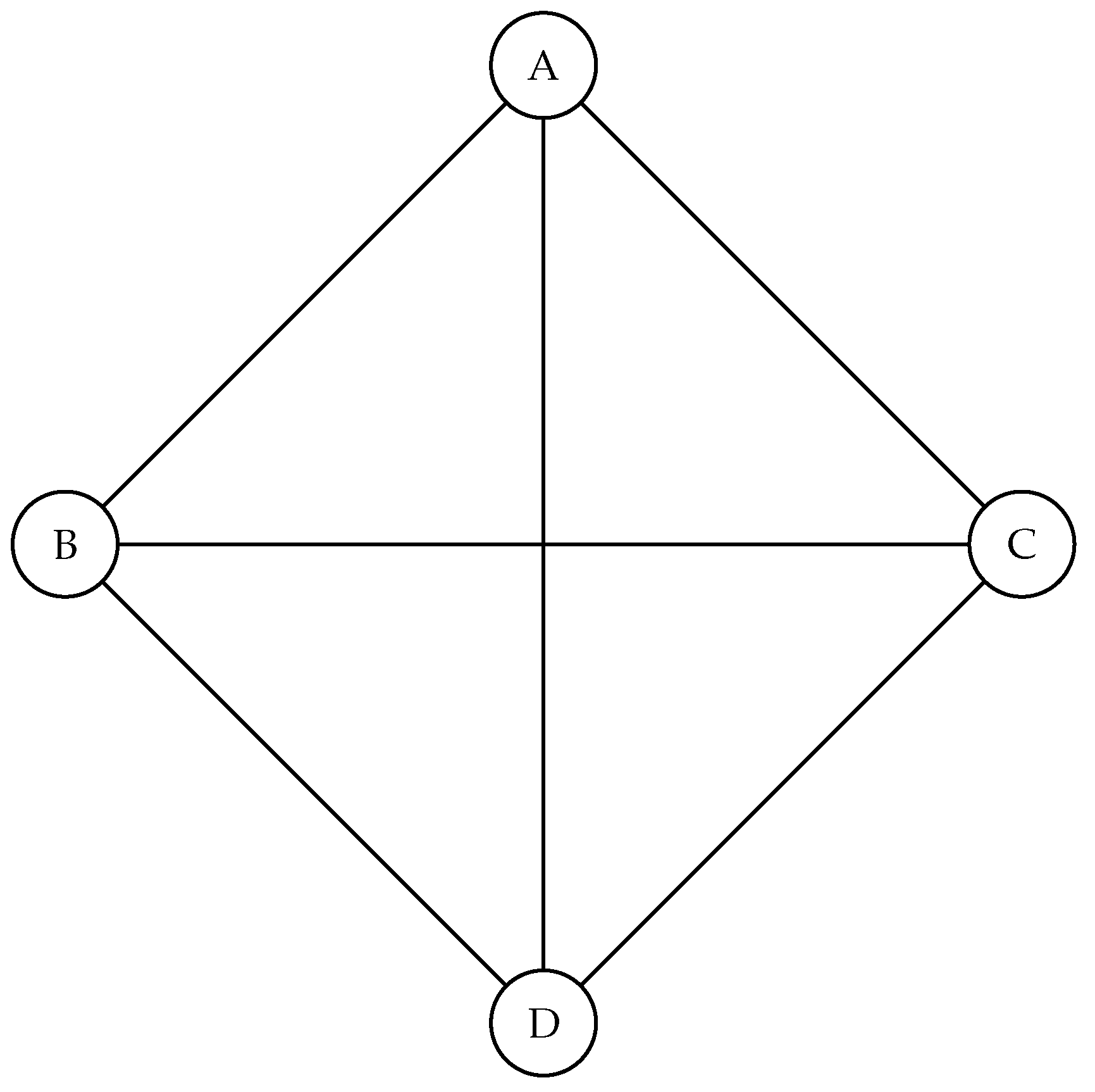
In the following graph Figure 2, a salesman has to visit all the cities named A, B, C and D. The problem entails finding the cheapest airline tickets and least travel time.
The Traveling Salesman Problem comes in two flavors: symmetric and asymmetric. The former can be modeled as a complete undirected graph , and the latter as a directed graph . Assuming that n denotes the number of cities (nodes), is the set of vertices, is the set of edges, and is the set of arcs. A cost matrix , which satisfies the triangle inequality for every , is defined for each edge or arc. In particular this is the case for problems where the vertices are points of the Euclidean plane, and is the Euclidean distance. The triangle inequality holds if the quantity represents the length of the shortest path from i to j in the graph G [6].
In the case of the symmetrical TSP, the number of all possible routes covering all cities and corresponding to feasible solutions is given by (recall that n stands for the number of cities). The Traveling Salesman Problem with Time Windows (TSP-TW) is a special case of the standard TSP in which the Traveling Salesman must pass through every city within a specific time interval (or “window”). This requirement imposes a rather strict additional time restriction. As expected, in this case not every TSP solution is automatically also a TSP-TW solution. As a consequence, the issue has become even intractable in reality. Indeed, in the standard TSP one can recognize an elegant symmetry in the sense that every permutation of cities is a viable solution. This symmetry is broken in the TSP-TW and, regrettably, even finding an initial admissible solution becomes very difficult [7]. Typically, in the TSP-TW the following input data are given: (i) a collection of cities (also referred to as customers), (ii) a specific customer called the depot, (iii) the service time to be spent on each customer, and (iv) the time window of each customer (i.e., the start time and the expiry time). Our task then is to compute the minimum cost path that begins and ends at the depot, such that each customer is visited before its expiry time.
Note that in the TSP-TW case how the depot is determined is critical, something that obviously does not hold in the standard TSP. We clarify that the Traveling Salesman is permitted to arrive at a customer before it is ready, resulting in unavoidable waiting. There are, of course, paths that prohibit the Traveling Salesman from complying with the time window of every customer. Those paths are referred to as infeasible, and those that permit full compliance with the time window of every customer are referred to as feasible paths. The complete range covered is the cost of the route.
2.2. Research on Algorithms for TSP and TSP-TW
Solving concrete, practical problems through CO techniques has always been a major goal in this field. Recently, many researchers have been actively seeking to improve on the standard methods of optimization by incorporating concepts and techniques derived from unconventional computing in an attempt to gain significant improvements. For instance, Talbi et al. [8] presented a new quantum inspired genetic algorithm for solving the TSP. Results of the proposed algorithm were found to be better than the ones obtained by standard genetic algorithms. Ascheuer et al. [9] addressed the asymmetric TSP-TW by implementing codes that were founded on three alternative integer programming formulations and more than ten heuristics. Papalitsas et al. [4] presented a General Variable Search heuristic that computes initial and feasible solutions for the TSP-TW. More importantly, the authors provided all the information relevant to TSP-TW, VNS and initialization methods. Gutin and Punnen [10] focused on the main algorithm’s behavior to sorting-based initialization procedures. The authors argued that the best way of finding solutions is understanding the algorithmic behavior since this would lay the foundations for determining the best solution out of those available. Finally, Jones and Adamatzky [11] demonstrated experimentally that using a sorting function as a standard function within their algorithm was not functional, and did fail to return a feasible solution in some of the cases.
Wang et al. [12] proposed an improved quantum inspired evolutionary algorithm (IQEA) for solving the TSP with Time Windows. Wu and Bao [13] contend that it is a hybrid algorithm of greed heuristics and quantum inspired evolutionary algorithm. The authors argue that the quantum inspired immune clonal algorithm is an emerging algorithm with vast potential for TSP-TW. Founded on the evolutionary game theory, the algorithm can solve a combination of optimization problems. Results from the study suggested that the proposed approach plays a crucial role in maintenance of good diversity, and attainment of superior performance. Chiang et al. [14] proposed a quantum inspired evolutionary algorithm (QEA), a quantum inspired Tabu search (QTS), which is founded on the classical Tabu search and quantum computation characteristics like superposition.
Da Cruz et al. [15] remark that evolutionary algorithms have been used for solving problems in diverse research fields since being put forth as an optimization method. Their success is attributed to the fact that they do not need prior information about the problem for them to be optimized and provide a high level of parallelism. Their results indicated that the algorithm could achieve better solutions when compared to other similar algorithms by significantly minimizing the time for convergence. Platel et al. [16] also argued that QEA applies various quantum computing principles for solving optimization problems. The paper established that QEA is an original algorithm belonging to the estimation class of distribution algorithms.
3. A GPS Application for Garbage Trucks Expressed as a TSP with Time Windows
Routing garbage trucks from the collection points to all dustbins on their routes is an important operation for the management of the day-to-day scheduling of the traffic of a city. Optimal routes are those that guarantee the minimum distance and transportation time. Unfortunately, finding optimal routes is time-consuming, particularly in metropolitan cities that have dense road networks. In contrast, through the exploitation of recent advances in the metaheuristics field, it is now possible to achieve efficient and almost optimal solutions within a short period for various practical cases. Our approach takes advantage of the improvement that can be gained by using the VNS metaheuristic procedure. The GVNS, taking into account the minimal computational time needed, could offer a better practical solution for such problems. Incorporating the improved VNS in the GIS should lead to the reduction the overall response time of the system and offer near-optimal solutions. Ideally, GIS technology tends to embed database operations like statistical and query analysis with the distinct geographic and visualization benefits that maps provide [17]. GIS enhances the spatial modeling of the network, enabling algorithms to assess and analyze its topology. Graphs are used for modeling spatial networks; arcs represent road segments, while nodes represent street segment intersections. Each arc encodes the cost of traversing it, as symbolized by the weight associated to it. A GIS normally offers various tools for analyzing spatial networks. It mainly provides tools for finding the minimum or shortest route via a network as well as heuristic procedures for finding the most efficient routes to various locations. Such problems are normally modeled as TSP instances. This implementation solves the TSP problem in an efficient way, and finds almost perfect solutions for various benchmark instances. Distance matrix calculations enable the computation of distances between nodes that represent destinations and origins, while allocation-location functions ascertain site locations, at the same time assigning demand to sites. These GIS capabilities for the analysis of spatial networks facilitate their use as decision support systems for vehicle routing [18]. The focus of this paper is finding near optimal solutions for the TSP-TW problem. Specifically, we will tackle the issue of garbage vehicle routing with time windows for solid waste collection. This work is inspired by our previous effort to treat the general garbage collection scenario by modeling it as the Travelling Salesman Problem [19]. As no polynomial time algorithm is expected for finding solutions to any form of the TSP, Keenan et al. [18] contend that one of the most popular approaches is the heuristics approaches. There are variations among heuristics in terms of performance, implementation difficulty and computation time.
To route a garbage truck from the depot to all dustbins and re-route it back, it is necessary to find the corresponding routes of the underlying TSP. The GIS will play a critical role in finding near optimal paths that approximate the minimum time needed for transportation. The GIS could also direct the driver to the generated routes. Transmission of the directions will be done to the garbage truck. How the routing is accomplished with respect to time constraints is quite crucial in this real-time system, and this could be guaranteed by metaheuristics. In this paper, we give a description of a system solving the garbage truck routing management problem. The basic ingredient of this solution is the quantum inspired metaheuristic that is applied to the TSP and is embedded to GPS/GIS. The approach used is a solution based on integrated waste management. Taking into account functional requirements and related studies (such as Asimakopoulos et al. [20]), the components of the application are constructed by smaller functional units and subsystems. For every subsystem, its operations and its relationships with the other subsystems are defined.
Bin Sensors are the equipment that provides an estimation of the waste bin fill level. This is critical for collecting, storing, and transmitting data regarding each bin. The main idea is to deliver the information that has been collected from the sensors to the central system. There are three components that can be installed on vehicles. The first component is the communicator responsible for the communication with the bin, the second is the storage procedure that stores data until it is transferred to the central system, and the third is the transfer procedure which rolls out data from the central system.
The Global System for mobile communication network will be used for applying all these operations: GPS navigation apps embedded in trucks, a central system, a map substructure, a data mining subsystem, and a routing optimization structure. The central system is the back-end system of our case study. All the spatial information generated for the route will be stored there. Also, data storage will entail information obtained/retrieved from other subsystems. A data mining subsystem is one used for estimating the bin’s fullness when there is lack of updated information. This work advocates a routing optimization structure as a major component that can offer optimal or near-optimal solutions over a short period.
Through the implementation of routing capabilities, a comparative advantage with respect to similar other attempts is noticed. Since this project is using a real-time system, it should have the capacity to provide prompt responses to such problems in view of the fact that the response period is quite important. Through the deployment of local search structures as well as GVNS for the problem, better results can be expected.
In this scenario that deals with time windows, each dumpster must be visited within a specific time frame. The experimental comparison corroborates the assumption that GVNS leads to results that are quite promising. Due to these improved routing solutions, lower amount of fuel is used. Consequently, the proposed method is also environmentally-friendly because fuel consumption directly affects the environment. From this foregoing, it is worth noting that this paper’s use of routing functionality is better than other methods due to two basic reasons. First, efficient solutions could be computed in a short period, thus making the application efficient since computation and re-computation can be repeatedly done for the same route. Secondly, this paper’s routing algorithm performs better than other classic methods including the NN [19], which are utilized for finding routes on GPS. As a result, the solutions obtained for all instances are very close to the optimal ones.
4. The Proposed Methodology
The garbage collection problem becomes more complex when garbage trucks are allowed to access certain bins only for some specific time frames during the day. A typical example of this situation happens in Corfu which is located in Greece. This irregularity is caused by the tourist period and the periodic traffic regulations imposed on some streets for specific hours during the day. Additionally, the old city of Corfu is an UNESCO monument characterized by great distinctiveness in terms of spatial planning and accessibility. Faithfully modeling this situation, transforms the classic garbage collection problem into a garbage collection problem with time windows. This scenario, from an algorithmic perspective, is adequately abstacted as the Traveling Salesman Problem with Time Windows.
In the rest of the paper we describe the approach we adopted to tackle the problem by utilizing the metaheuristic Variable Neighborhood Search. For a comprehensive assessment we present both a classic approach as well as a quantum inspired procedure for solving this problem.
4.1. Variable Neighborhood Search
Variable Neighborhood Search (VNS), proposed by Mladenovic and Hansen, is a metaheuristic designed for tackling combinatorial and global optimization [21,22] problems. The primary concept of this structure is a systematic shift of neighborhoods in an effort to arrive at an optimal (or close-to-optimal) solution [23]. VNS and its many extensions have demonstrated their effectiveness in addressing a number of combinatorial and global optimization problems [24,25]. A VNS heuristic is made up of three ingredients. The first is the shaking process (diversification phase) used to evade solutions that are only locally optimal. The second is the neighborhood change move, which establishes the next neighborhood that should be examined; in this part, the approval or refusal criterion is also applied to the last solution found. The third part is the improvement phase (intensification), which is accomplished through the traversal of the neighborhood structures using various local search movements. This exploration is primarily carried out by one of the following neighbourhood shift phases:
- Cyclic neighbourhood shift phase: whether or not there is an enhancement with regard to the present alternative, the search proceeds to the next neighbourhood structure in the list.
- Pipe neighbourhood shift phase: if there is an enhancement of the present solution in some neighbourhood, the exploration will continue in that neighbourhood.
- Skewed neighbourhood shift step: recognize as new incumbent solutions not only enhancing solutions but also some of those that are worse than the present incumbent solution. The aim of such a neighborhood change step is to permit the exploration of valleys far from the current solution. The solution of the current trial must be assessed considering not only the objective values of the trial and the incumbent solution, but also the distance between them.
Variable neighborhood search variants. Many variants of VNS have been developed and applied for solving hard optimization problems [26]. The Basic VNS (BVNS), the Variable Neighborhood Descent (VND), the General VNS (GVNS), and the Reduced VNS (RVNS) are the most commonly used variants. In the BVNS a diversification method and a local search operator are alternated. VND consists of an improvement procedure in which the neighborhood structures are explored systematically, and a neighborhood change step. There are different VND variants according to their neighborhood change step. The pipe-VND, which uses the pipe neighborhood change step, seems to be the most efficient method for the solution of computationally challenging problems [26]. General Variable Neighborhood Search (GVNS) is a VNS variant where a VND method is used as the improvement procedure. GVNS has been successfully tested in many applications, as several recent works have demonstrated [27,28].
4.2. Our Approach
This work studies the implementation of a GVNS metaheuristic for the TSP-TW that is inspired by the method described in [29]. In addition to the aforementioned conventional approach, we propose an unconventional GVNS scheme that solves the TSP with Time Windows using quantum inspired principles on the perturbation function. For those two separate implementations we also followed [30,31]. In this paragraph the design and implementation process will be discussed. The overview explained here is using the technique outlined in [29] that was designed for the TSP with time windows.
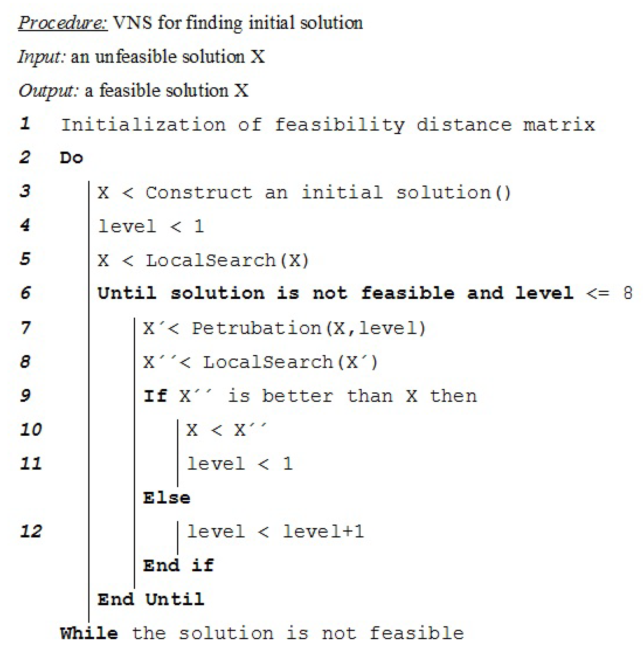
The method in Figure 3 is the main one and focuses on discovering a feasible solution by using GVNS. First of all, in line 1 we create a table that demonstrates (before the algorithm begins) which nodes are reachable from each other and which are not, taking into account the limitations imposed by the time windows and particularly the due time of the visited node. The core algorithm utilizes this method to exclude the possibility of reviewing paths that do not satisfy the time limitations. The method from line 2 to the end is reiterated until a feasible solution is discovered. A random or sorted solution is produced in the third row. The level is set to 1 in row four. The level controls the number of repetitions of the shake function. The shake function is responsible for escaping the current local minimum and accepting the produced solution. The highest level is 8 because it has been experimentally determined that this is the best value [29]. The first local search is conducted before the loop execution begins in case the problem can be solved immediately. The primary loop is executed while the variable level is less than 8 and an admissible solution has not been discovered. Inside the loop, a disordered solution is determined on the basis of the level value. At this point, if the new solution constructed after a local search is conducted, is better than the present one, we set it as the present preferred solution. If a new best solution is discovered, we will set the level to 1. If the solution after the local search is not better than the present one, then we enhance the value of the level parameter and proceed to the next cycle. We emphasize that the best solution is the one with the least number of violated nodes. If two solutions have the same number of violated nodes, we keep the best solution, that is the one with the least cost. We recall that a node is violated if it visited after its expiry time. The individual subroutines of the GVNS are described below.
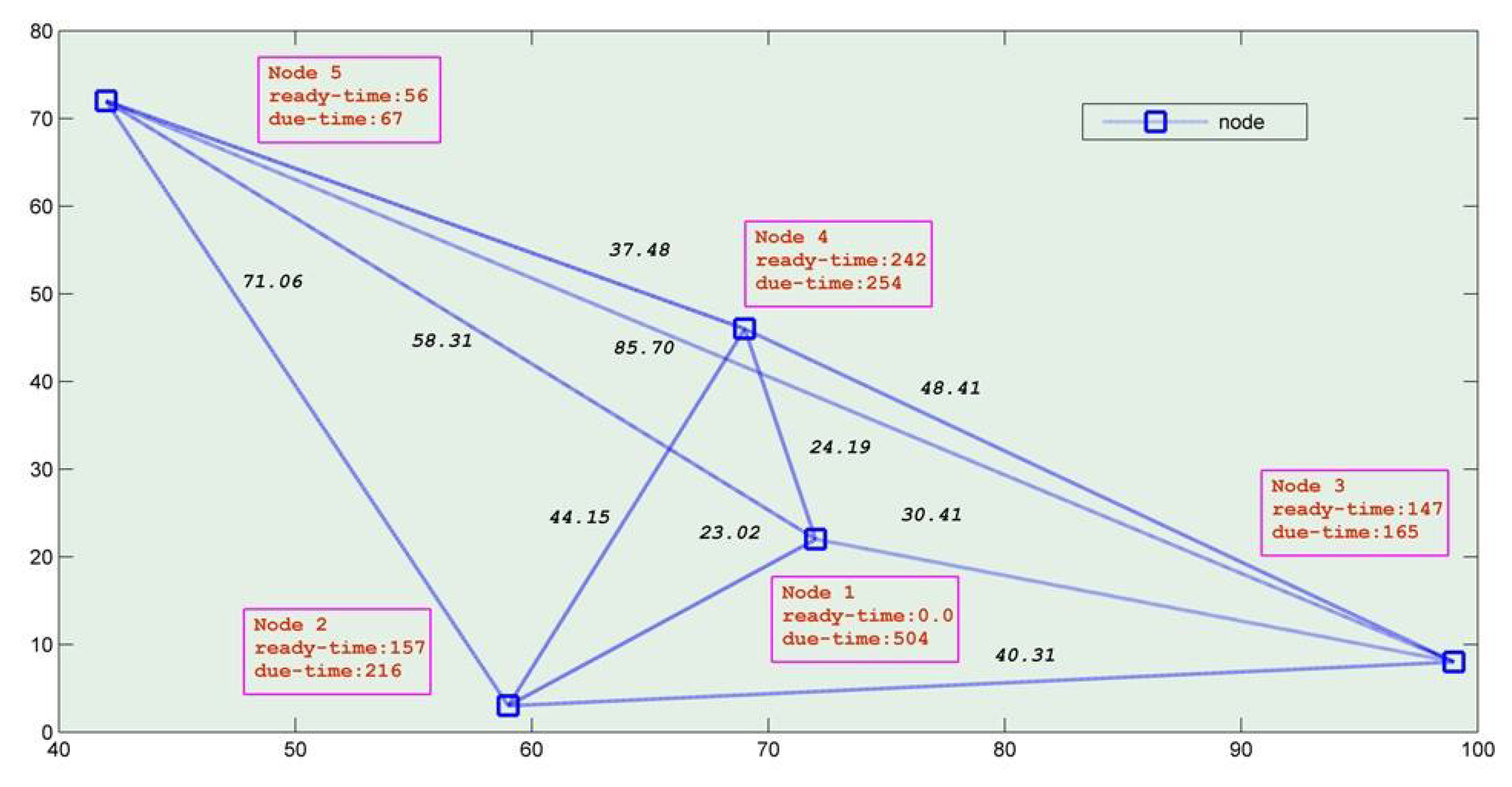
Figure 4 depicts a simple illustrated example of a TSP-TW showing with specific data values the simple modeling of the problem.
4.3. Perturbation, Neighborhood Structures
Local search is performed using a 1-shift method as a neighborhood structure. This approach is intended to improve the current solution by moving some nodes along with others in the sequence. If the current solution is not feasible, two types of nodes emerge: the violated nodes (those visited after due time) and the non-violated nodes (those nodes visited before due time). Consequently, the main neighborhood may be separated into two new sub-neighborhoods; in the first neighborhood, the movements consist of violated nodes, and in the second neighborhood of non-violated nodes. The existence of two neighborhoods implies that care must be given to the order of their exploration. The optimal order of neighborhood investigation is given below [29]:
- Move backwards the violated nodes back,
- Move forward the non-violated nodes,
- Move the non-violated nodes backwards, and
- Move forward the violated nodes.
This order performs better than others, where the term “better” is interpreted as the combination of neighborhoods that produces a feasible solution more quickly. The perturbation function process is used as a local minimum-shaking function-entrapment prevention procedure. In our execution, the algorithm conducts random node shifts (1-shifts) to some randomly chosen nodes in the present solution without taking into consideration any control condition to move to a better solution [4].
4.4. Quantum Inspired Perturbation
Quantum-inspired methods use concepts of quantum computing. Quantum computing is a field introduced relatively recently (in the 1980s) by Feynman, who said that effective simulation of an actual quantum system using a classical computer is not possible as there would be an exponential slowdown in the simulation of actual quantum processes [32,33].
The qubit is the quantum analogue of the classical bit. Similarly, the quantum register, which is a collection of qubits, is the quantum analogue of the classical processor register. In each call of this shaking method, a simulated quantum n-qubit register generates a normalized complex n-dimensional unit vector. In this context, normalized means that, if is the complex vector, then . The dimension n of the complex unit vector is greater than or equal to the dimension of the problem. The complex n-dimensional vector is converted into a real n-dimensional vector, the components of which are real numbers in the interval . If and are the ith components of the complex and real vectors respectively, then , i.e., is equal to the modulus squared of . Moreover, each of the real vector’s selected components corresponds to a current solution node.
Each node of the current solution uses the components as a flag. Sorting the first vector impacts the order in the solution vector owing to the correspondence in a tour between components and nodes, driving the exploration effort to another stage in the search space. That’s our third algorithm’s shaking technique [31].
5. Computational Results
5.1. Implementation Technology and Instances Used
Our implementation has been coded in JAVA. An important reason for choosing JAVA, is that to the best of our knowledge there exists no object-oriented implementation for this specific optimization problem. Furthermore, JAVA is a well known language, hence our algorithm will be accessible to a wide audience.
We tested all three different variants, including symmetrical instances, with different benchmark problems proposed by [34,35]. Each benchmark problem’s name has the following structure; letter n (i.e., number), followed by real amount of customers. Then, letter w (i.e., maximum window width) followed by the highest window length value. The file name n20w100 codes a problem with 20 clients and a maximum window length of 100.
5.2. Computational Results on Known Benchmarks
In this section we present the extensive comparative study of three different variations of our GVNS heuristic. The first one starts with a random solution while the main body of this procedure tries to improve our solution via four different variations of 1-shift heuristic. The second implementation starts with a sorted solution while using the same 1-shift heuristic (once again by producing four different movement by using the 1-shift heuristic). The third one starts with a quantum inspired method on the initial input while the improvement phase is still the same 1-shift based. The perturbation method is inspired from quantum computing.
Below, we present the computational results for the three separate variations of the GVNS scheme on some well-known benchmarks. Specifically, the computational results are presented in two tables, Table 1 and Table 2. A comparative study of the RSC GVNS variant and the QISC is shown at Table 1, and a similar comparison between the SSC conventional GVNS and the QISC is given in Table 2. The QISC results in both tables Table 1 and Table 2 are shown in bold since we wanted to emphasize the superiority of the quantum inspired variation for particular instances of the benchmarks. To this end, we highlight in Table 1 that in five out of ten in total benchmarks QISC produces better result than RSC, while in Table 2 QISC outperforms SSC on nine out of ten in total benchmarks. Table 3 includes all required abbreviations.
5.3. A Practical Test Case with Real Data
A practical case study where garbage collection with time windows can be applied, is the case study of city of Corfu, Greece. Corfu is particularly crowded during the summer season due to the extremely high tourist activity. As a consequence, many roads which are to be used by vehicles are closed and only pedestrians are allowed to pass for a specific time frame. So, those roads have a ready and due time for garbage trucks to have access there. This problem can be modeled as garbage collection with time windows and can be treated by solving the TSP with Time Windows.
We constructed the data set, which serves as a real world problem benchmark, with route information from Corfu and with routing information of the garbage trucks from the recycling station to each bin location and back to recycling station (depot), by using Google’s Direction API. The Directions API [36] is a service that calculates distances between locations using an HTTP request. This API provides many usage options to the user. On may inquire for directions for several modes of transportation, such as transit, driving, walking or cycling. Moreover, it can return multi-part directions using a series of waypoints. It can specify origins, destinations, and way-points as text strings, or as latitude/longitude coordinates, or as place IDs.
We have used all the above information in order to construct the tour of a garbage truck that has as a depot the recycling center of Corfu town, and a tour with nodes to some of the most important places where recycling dumpsters are located. To complete our example we have added time limitations regarding the visiting time of each node, as needed in order to fully simulate this problem. We have run this new real world problem using our quantum inspired version of the solver since it seems to provide better solutions than the other two conventional variations.
Our benchmark consists of 21 nodes, a depot (where the recycling center is located) and 20 nodes where recycling dumpsters are being placed. The coordinates of each node are listed in Table 4.
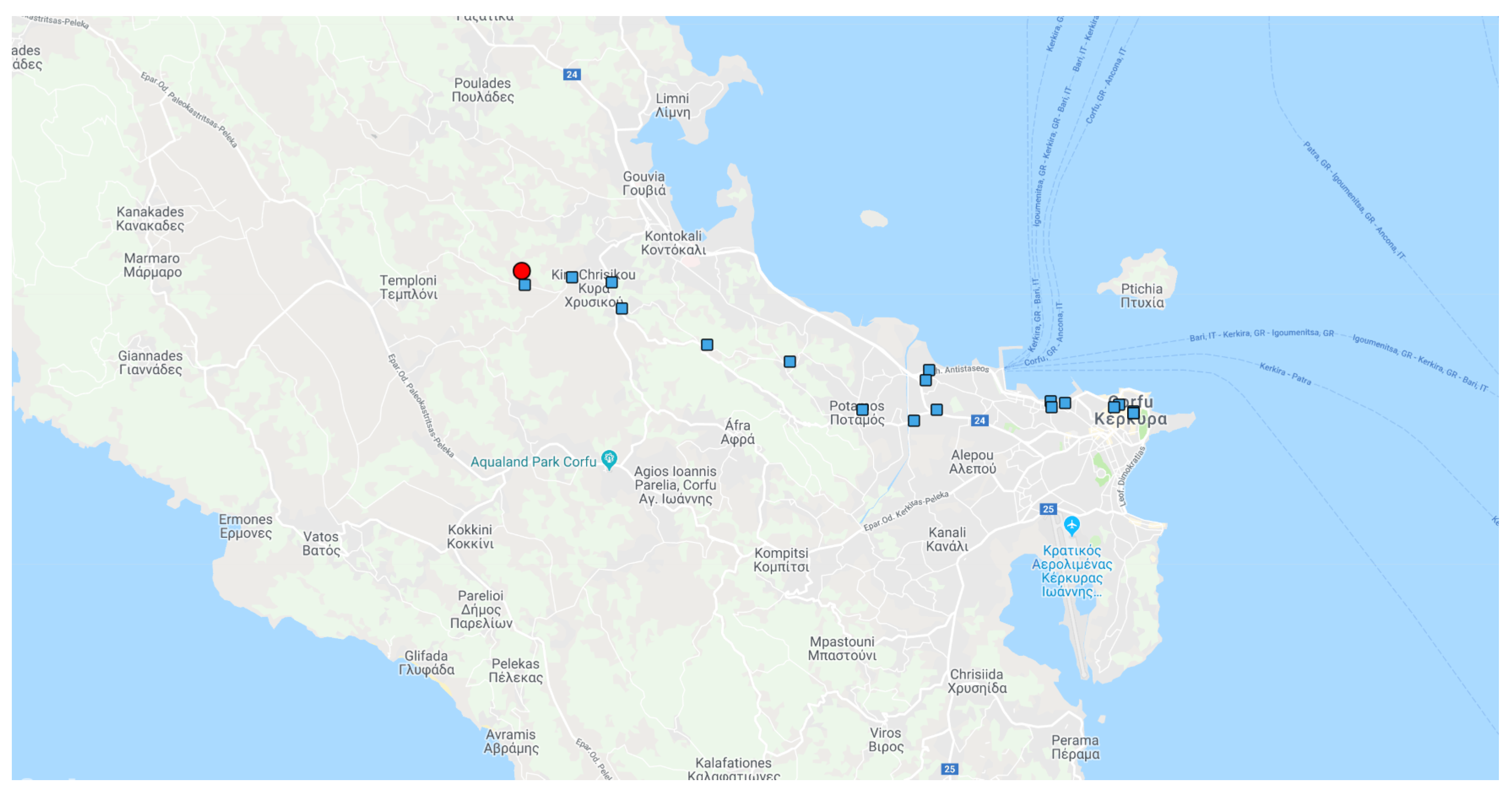
In addition to the above Table 4, we present the following graphic depiction in Figure 5, extracted from maps, showing where the depot and the other nodes are located so as to better illustrate the specific problem.
Using this benchmark as an input to our quantum inspired implementation, we have found out a feasible solution for our benchmark. The order of the nodes after the execution is the following: [0, 6, 2, 11, 19, 3, 4, 8, 5, 14, 15, 10, 9, 7, 20, 13, 18, 16, 0, 12, 17, 1], and the resulting cost of the produced solution is 319.0. The above results are quite promising and encourage us to apply our research on alternative optimization models to other real world problems as well.
6. Conclusions
This work studies the application of garbage collection routing with additional limitations on the time that every node is available to be visited by the garbage truck. The preferred method is a metaheuristic that is based on a novel quantum inspired variation of the GVNS. The underlying problem was modeled as a TSP with Time Windows, and solved by using a General Variable Neighborhood search variation. Due to our utilization of quantum computation methods, our metaheuristic differs from conventional approaches. In order to conduct an assessment of the efficiency of the approach, extensive experimental tests were carried out using established benchmarks.
Future work should include further investigation of alternative neighborhood structures usage, as well as neighborhood change in variable neighborhood descent under the GVNS framework. Similarly, one can explore modifications in the shaking function as a way of achieving better solutions, especially on larger benchmarks. Another venue to explore can be the deployment of a multi-improvement strategy. Finally, the application of our algorithm to other real world problems will be a direction for our next research steps.
Author Contributions
All authors have contributed substantially to this work.
Funding
This research received no external funding.
Conflicts of Interest
The authors declare no conflict of interest.
References
- Bonnans, J.F.; Shapiro, A. Perturbation Analysis of Optimization Problems; Springer Science & Business Media: Berlin, Germany, 2013. [Google Scholar]
- Feillet, D.; Dejax, P.; Gendreau, M. Traveling Salesman Problems with Profits. Transp. Sci. 2005, 39, 188–205. [Google Scholar] [CrossRef]
- Cheng, C.B.; Mao, C.P. A modified ant colony system for solving the travelling salesman problem with time windows. Math. Comput. Model. 2007, 46, 1225–1235. [Google Scholar] [CrossRef]
- Papalitsas, C.; Giannakis, K.; Andronikos, T.; Theotokis, D.; Sifaleras, A. Initialization methods for the TSP with Time Windows using Variable Neighborhood Search. In Proceedings of the 6th International Conference on Information, Intelligence, Systems and Applications (IISA 2015), Corfu, Greece, 6–8 July 2015. [Google Scholar]
- Voigt, B.F. Der Handlungsreisende, Wie er Sein Soll und was er zu Thun hat, um Aufträge zu Erhalten und Eines Glücklichen Erfolgs in Seinen Geschäften Gewiss zu zu Sein; Commis-Voageur: Ilmenau, Germany; Neu Aufgelegt Durch Verlag Schramm: Kiel, Germany, 1981. [Google Scholar]
- Johnson, R.; Pilcher, M.G. The Traveling Salesman Problem; Lawler, E.L., Lenstra, J.K., Kan, A.H.G.R., Shmoys, D.B., Eds.; John Wiley & Sons: Chichester, UK, 1985; 463p. Networks 1989, 19, 615–616. [Google Scholar] [CrossRef]
- Savelsbergh, M.W. Local search in routing problems with time windows. Ann. Oper. Res. 1985, 4, 285–305. [Google Scholar] [CrossRef] [Green Version]
- Talbi, H.; Draa, A.; Batouche, M. A new quantum-inspired genetic algorithm for solving the travelling salesman problem. In Proceedings of the 2004 IEEE International Conference on Industrial Technology, 2004. IEEE ICIT’04, Hammamet, Tunisia, 8–10 December 2004; Volume 3, pp. 1192–1197. [Google Scholar]
- Ascheuer, N.; Fischetti, M.; Grötschel, M. Solving the Asymmetric Travelling Salesman Problem with time windows by branch-and-cut. Math. Program. 2001, 90, 475–506. [Google Scholar] [CrossRef]
- Gutin, G.; Punnen, A.P. The Traveling Salesman Problem and Its Variations; Springer Science & Business Media: Berlin, Germany, 2006; Volume 12. [Google Scholar]
- Jones, J.; Adamatzky, A. Computation of the Travelling Salesman Problem by a Shrinking Blob. Natural 2014, 13, 1–16. [Google Scholar] [CrossRef]
- Wang, L.; Kowk, S.; Ip, W. Design of an improved quantum-inspired evolutionary algorithm for a transportation problem in logistics systems. J. Intell. Manuf. 2012, 23, 2227–2236. [Google Scholar] [CrossRef]
- Wu, Y.; Bao, J.J. New mixed quantum-inspired evolutionary algorithm for TSP. J. Comput. Appl. 2006, 10, 2433–2436. [Google Scholar]
- Chiang, H.P.; Chou, Y.H.; Chiu, C.H.; Kuo, S.Y.; Huang, Y.M. A Quantum-inspired Tabu Search Algorithm for Solving Combinatorial Optimization Problems. Soft Comput. 2014, 18, 1771–1781. [Google Scholar] [CrossRef]
- da Cruz, A.A.; Vellasco, M.M.B.R.; Pacheco, M.A.C. Quantum-inspired evolutionary algorithm for numerical optimization. In Hybrid Evolutionary Algorithms; Springer: Berlin, Germany, 2007; pp. 19–37. [Google Scholar]
- Platel, M.D.; Schliebs, S.; Kasabov, N. Quantum-inspired evolutionary algorithm: A multimodel EDA. IEEE Trans. Evol. Comput. 2009, 13, 1218–1232. [Google Scholar] [CrossRef]
- Muller, J.C. Guest Editorial Latest developments in GIS/LIS. Int. J. Geogr. Inf. Syst. 1993, 7, 293–303. [Google Scholar] [CrossRef]
- Keenan, P.B.; Jankowski, P. Spatial Decision Support Systems: Three decades on. Decis. Support Syst. 2019, 116, 64–76. [Google Scholar] [CrossRef]
- Papalitsas, C.; Karakostas, P.; Andronikos, T.; Sioutas, S.; Giannakis, K. Combinatorial GVNS (General Variable Neighborhood Search) Optimization for Dynamic Garbage Collection. Algorithms 2018, 11, 38. [Google Scholar] [CrossRef]
- Asimakopoulos, G.; Christodoulou, S.; Gizas, A.; Triantafillou, V.; Tzimas, G.; Gialelis, J.; Voyiatzis, A.; Karadimas, D.; Papalambrou, A. Architecture and Implementation Issues, Towards a Dynamic Waste Collection Management System. In Proceedings of the 24th International Conference on World Wide Web, Florence, Italy, 18–22 May 2015; ACM: New York, NY, USA, 2015; pp. 1383–1388. [Google Scholar] [CrossRef]
- Mladenovic, N.; Hansen, P. Variable neighborhood search. Comput. Oper. Res. 1997, 24, 1097–1100. [Google Scholar] [CrossRef]
- Hansen, P.; Mladenovic, N.; Todosijevic, R.; Hanafi, S. Variable neighborhood search: Basics and variants. EURO J. Comput. Optim. 2016, 5, 423–454. [Google Scholar] [CrossRef]
- Mladenovic, N.; Todosijevic, R.; Uroševic, D. Less is more: Basic variable neighborhood search for minimum differential dispersion problem. Inf. Sci. 2016, 326, 160–171. [Google Scholar] [CrossRef]
- Jarboui, B.; Derbel, H.; Hanafi, S.; Mladenovic, N. Variable neighborhood search for location routing. Comput. Oper. Res. 2013, 40, 47–57. [Google Scholar] [CrossRef]
- Karakostas, P.; Sifaleras, A.; Georgiadis, C. Basic VNS algorithms for solving the pollution location inventory routing problem. In Proceedings of the 6th International Conference on Variable Neighborhood Search (ICVNS 2018), Sithonia, Greece, 4–7 October 2018; Sifaleras, A., Salhi, S., Brimberg, J., Eds.; Springer: Berlin, Germany, 2019; Volume 11328. [Google Scholar]
- Karakostas, P.; Sifaleras, A.; Georgiadis, C. A general variable neighborhood search-based solution approach for the location-inventory-routing problem with distribution outsourcing. Comput. Chem. Eng. 2019, 126, 263–279. [Google Scholar] [CrossRef]
- Sifaleras, A.; Konstantaras, I.; Mladenović, N. Variable neighborhood search for the economic lot sizing problem with product returns and recovery. Int. J. Prod. Econ. 2015, 160, 133–143. [Google Scholar] [CrossRef]
- Sifaleras, A.; Konstantaras, I. General variable neighborhood search for the multi-product dynamic lot sizing problem in closed-loop supply chain. Electron. Notes Discret. Math. 2015, 47, 69–76. [Google Scholar] [CrossRef]
- Da Silva, R.F.; Urrutia, S. A General VNS heuristic for the traveling salesman problem with time windows. Discret. Optim. 2010, 7, 203–211. [Google Scholar] [CrossRef] [Green Version]
- Mladenović, N.; Todosijević, R.; Urošević, D. An efficient GVNS for solving traveling salesman problem with time windows. Electron. Notes Discret. Math. 2012, 39, 83–90. [Google Scholar] [CrossRef]
- Papalitsas, C.; Karakostas, P.; Kastampolidou, K. A Quantum Inspired GVNS: Some Preliminary Results. In GeNeDis 2016; Vlamos, P., Ed.; Springer International Publishing: Cham, Switzerland, 2017; pp. 281–289. [Google Scholar]
- Feynman, R.P. Simulating physics with computers. Int. J. Theor. Phys. 1982, 21, 467–488. [Google Scholar] [CrossRef]
- Feynman, R.P.; Hey, J.; Allen, R.W. Feynman Lectures on Computation; Addison-Wesley Longman Publishing Co., Inc.: Boston, MA, USA, 1998. [Google Scholar]
- Calvo, R.W. A new heuristic for the traveling salesman problem with time windows. Transp. Sci. 2000, 34, 113–124. [Google Scholar] [CrossRef]
- Ohlmann, J.W.; Thomas, B.W. A compressed-annealing heuristic for the traveling salesman problem with time windows. INFORMS J. Comput. 2007, 19, 80–90. [Google Scholar] [CrossRef]
- Directions API. Available online: https://developers.google.com/maps/documentation/directions/start (accessed on 27 August 2019).
Figure 1.
A toy scale example of a tour consisting of 4 nodes.

Figure 2.
Example of a tour consisting of 4 nodes.

Figure 3.
Pseudocode of the Meta-heuristic [4].
Figure 3.
Pseudocode of the Meta-heuristic [4].

Figure 4.
A simple visual example of TSP-TW with 5 nodes [4].
Figure 4.
A simple visual example of TSP-TW with 5 nodes [4].

Figure 5.
The case study of the recycling garbage trucks of Corfu.


Table 1.
Computational Results- RSC vs. QISC comparative study.
| Name | N | Max WL | Best Sol. | Proposed by | RSC | Dif. from Best Sol. | QISC | Dif. from Best Sol |
|---|---|---|---|---|---|---|---|---|
| n20w120 | 20 | 120 | 265.6 | Ohlmann and Thomas (2007) | 357.49 | 34% | 354.03 | 33% |
| n20w140 | 20 | 140 | 232.8 | Ohlmann and Thomas (2007) | 337.05 | 44% | 306.88 | 32% |
| n20w160 | 20 | 160 | 218.2 | Ohlmann and Thomas (2007) | 331.00 | 51% | 390.72 | 79% |
| n20w180 | 20 | 180 | 236.6 | Ohlmann and Thomas (2007) | 336.58 | 42% | 365.64 | 54% |
| n20w200 | 20 | 200 | 241.0 | Ohlmann and Thomas (2007) | 365.87 | 51% | 365.36 | 51% |
| n40w120 | 40 | 120 | 360.0 | Calvo (2000) | 521.18 | 44% | 551.84 | 53% |
| n40w140 | 40 | 140 | 348.4 | Calvo (2000) | 493.35 | 41% | 518.36 | 49% |
| n40w160 | 40 | 160 | 326.8 | Ohlmann and Thomas (2007) | 482.20 | 47% | 552.24 | 69% |
| n40w180 | 40 | 180 | 326.8 | Calvo (2000) | 532.49 | 62% | 519.42 | 59% |
| n40w200 | 40 | 200 | 313.8 | Ohlmann and Thomas (2007) | 493.65 | 57% | 468.01 | 49% |
Table 2.
Computational Results- SSC vs. QISC comparative study.
| Name | N | Max WL | Best Sol. | Proposed by | SSC | Dif. from Best Sol. | QISC | Dif. from Best Sol |
|---|---|---|---|---|---|---|---|---|
| n20w120 | 20 | 120 | 265.6 | Ohlmann and Thomas (2007) | 371.78 | 39% | 354.03 | 33% |
| n20w140 | 20 | 140 | 232.8 | Ohlmann and Thomas (2007) | 370.61 | 59% | 306.88 | 32% |
| n20w160 | 20 | 160 | 218.2 | Ohlmann and Thomas (2007) | 398.08 | 82% | 390.72 | 79% |
| n20w180 | 20 | 180 | 236.6 | Ohlmann and Thomas (2007) | 418.13 | 76% | 365.64 | 54% |
| n20w200 | 20 | 200 | 241.0 | Ohlmann and Thomas (2007) | 414.70 | 72% | 365.36 | 51% |
| n40w120 | 40 | 120 | 360.0 | Calvo (2000) | 549.97 | 52% | 551.84 | 53% |
| n40w140 | 40 | 140 | 348.4 | Calvo (2000) | 563.83 | 61% | 518.36 | 49% |
| n40w160 | 40 | 160 | 326.8 | Ohlmann and Thomas (2007) | 553.81 | 69% | 552.24 | 69% |
| n40w180 | 40 | 180 | 326.8 | Calvo (2000) | 561.09 | 71% | 519.42 | 59% |
| n40w200 | 40 | 200 | 313.8 | Ohlmann and Thomas (2007) | 558.65 | 78% | 468.01 | 49% |
| Abbreviation | Full Name |
|---|---|
| N | Number of nodes |
| Max WL | Max Window Length |
| Best Sol | Best Solution |
| RSC | Random Solution Cost |
| RST | Random Solution Time |
| dif. from best sol. | Difference from best solution |
| SSC | Sorted Solution Cost |
| SST | Sorted Solution Time |
| QISC | Quantum Inspired Solution Cost |
Table 4.
Practical case’s data
| Node | Longitude | Latitude | Comment |
|---|---|---|---|
| 1 | 39.6422466 | 19.8223686 | the depot |
| 2 | 39.6404733 | 19.8229525 | a dumpster node |
| 3 | 39.6413691 | 19.8306238 | a dumpster node |
| 4 | 39.6407922 | 19.8370158 | a dumpster node |
| 5 | 39.6374761 | 19.8386927 | a dumpster node |
| 6 | 39.6329728 | 19.8526526 | a dumpster node |
| 7 | 39.6308208 | 19.8660169 | a dumpster node |
| 8 | 39.6246663 | 19.8778979 | a dumpster node |
| 9 | 39.6234445 | 19.8863486 | a dumpster node |
| 10 | 39.6247393 | 19.8899176 | a dumpster node |
| 11 | 39.6284544 | 19.8880917 | a dumpster node |
| 12 | 39.6297152 | 19.8887043 | a dumpster node |
| 13 | 39.6257976 | 19.9083606 | a dumpster node |
| 14 | 39.625156 | 19.9085661 | a dumpster node |
| 15 | 39.6243003 | 19.9219708 | a dumpster node |
| 16 | 39.6256647 | 19.9108012 | a dumpster node |
| 17 | 39.6262482 | 19.9179632 | a dumpster node |
| 18 | 39.6251191 | 19.9187309 | a dumpster node |
| 19 | 39.6254352 | 19.9195927 | a dumpster node |
| 20 | 39.6246342 | 19.9219791 | a dumpster node |
| 21 | 39.6243003 | 19.9219708 | a dumpster node |
© 2019 by the authors. Licensee MDPI, Basel, Switzerland. This article is an open access article distributed under the terms and conditions of the Creative Commons Attribution (CC BY) license (http://creativecommons.org/licenses/by/4.0/).
Share and Cite
MDPI and ACS Style
Papalitsas, C.; Andronikos, T. Unconventional GVNS for Solving the Garbage Collection Problem with Time Windows. Technologies 2019, 7, 61. https://doi.org/10.3390/technologies7030061
AMA Style
Papalitsas C, Andronikos T. Unconventional GVNS for Solving the Garbage Collection Problem with Time Windows. Technologies. 2019; 7(3):61. https://doi.org/10.3390/technologies7030061
Chicago/Turabian StylePapalitsas, Christos, and Theodore Andronikos. 2019. "Unconventional GVNS for Solving the Garbage Collection Problem with Time Windows" Technologies 7, no. 3: 61. https://doi.org/10.3390/technologies7030061
Note that from the first issue of 2016, this journal uses article numbers instead of page numbers. See further details here.