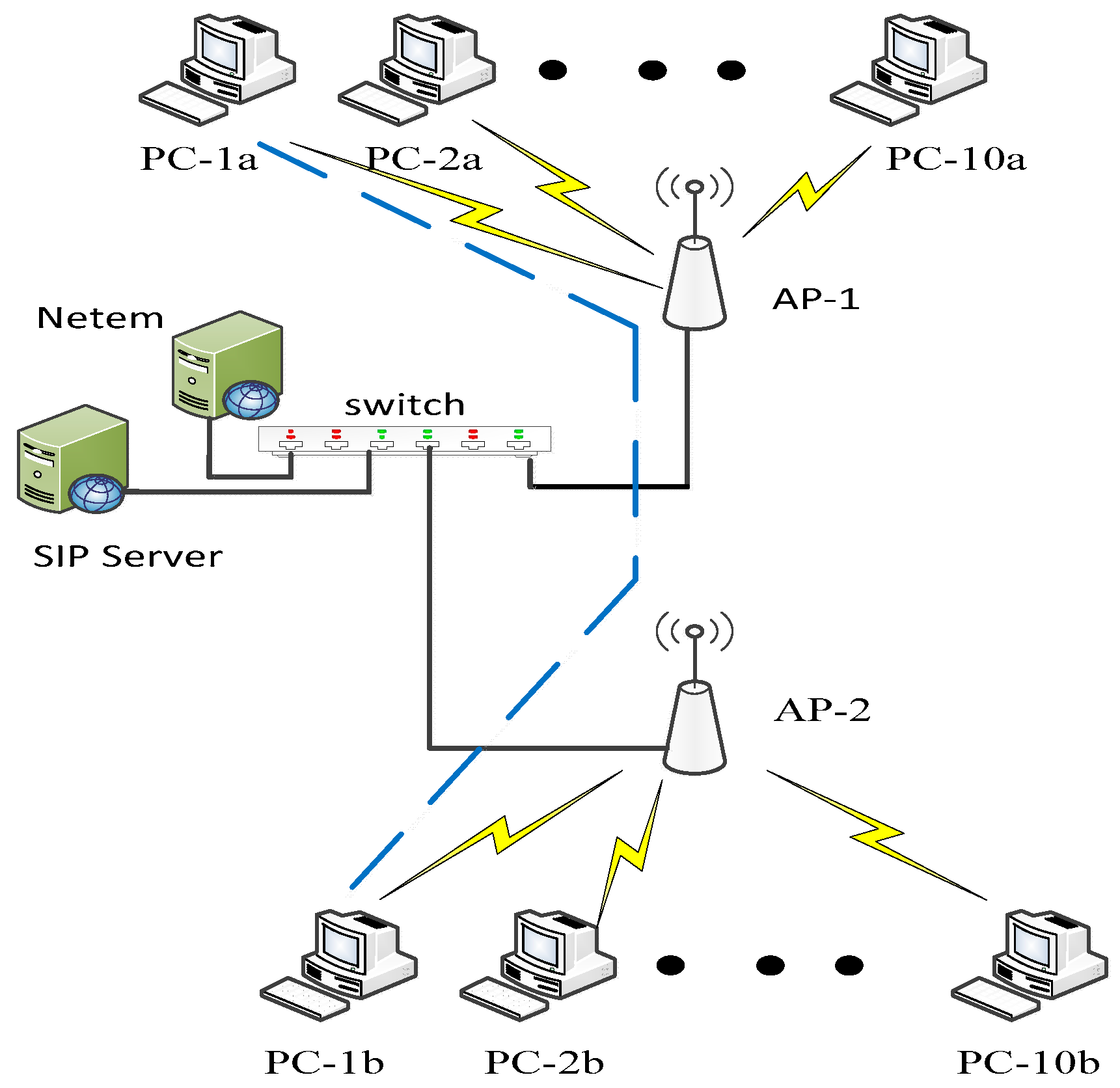
The network consisted of two Cisco
© AIR-AP1852E access points (APs) operating using the IEEE 802.11ac/n Wi-Fi protocol. Cisco
© APs contain four external dual-band antennas. A Cisco
© catalyst 3560-CX switch connected the two APs with a Session Initiation Protocol (SIP) server via 1 Giga bits per second (Gbps) wired links. The specifications of the personal computers (PCs) used in the study were as follows: Intel
© Core i7-3770 processor, 3.40 GHz, 16 GB DDR3 RAM, Microsoft Windows
© 7 Enterprise SP1 64 bits, for 802.11ac Linksys
© AC1200 Dual-Band wireless adaptor. There was no encryption activated between the APs and the PCs’ wireless adapters. As the wireless devices were close to each other, the transmission power was kept to 30 mW (15 dBm) [
24].
The traffic transmission lasted for up to three minutes and consisted of high-definition (HD) video using MPEG-2, Voice over Internet Protocol (VoIP), and data transmission using the Transmission Control Protocol (TCP). VoIP connectivity was established by Session Initiation Protocol (SIP) and used the Real-Time Transport protocol (RTP). X-Lite Softphones software ran over the Microsoft Windows© operating system providing SIP VoIP, using a G711a coder–decoder (CODEC), and RTP was used with a packet size of 160 bytes. The queuing mechanism for all scenarios was First-In-First-Out (FIFO) chosen for its simplicity, and queue size was 50 packets.
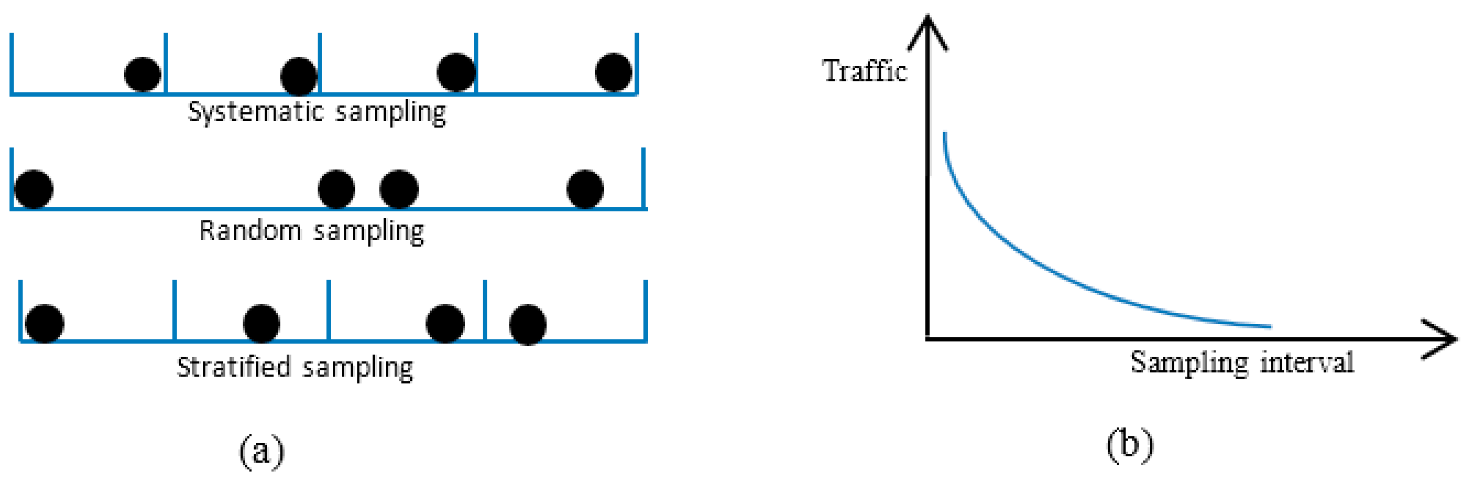
As a large number of packets were sent, sampling was needed to evaluate the QoS. An adaptive sampling technique was developed to select packets that best represented the original traffic.
Network Traffic Parameters
The Wireshark network monitoring captured RTP packets (installed on two of the PCs) that were sorted using their sequence numbers to determine end-to-end delay, jitter, and percentage packet loss ratio as outlined below [
27,
28,
29].
End-to-end delay was determined for each packet. For the
ith packet, the delay (
Di) was calculated by subtracting the arrival time for the packet (
) from the sent time (
) as indicated by Equation (1).
The magnitude of jitter (
Ji) was measured by determining the difference between the current packet delay (
) and the delay for the previous packet (
) as in Equation (2).
The percentage packet loss ratio (%PLR
i) was measured by determining the total number of received packets (
) and the total number of sent packets (
) at a given time (
t), as illustrated in Equation (3).
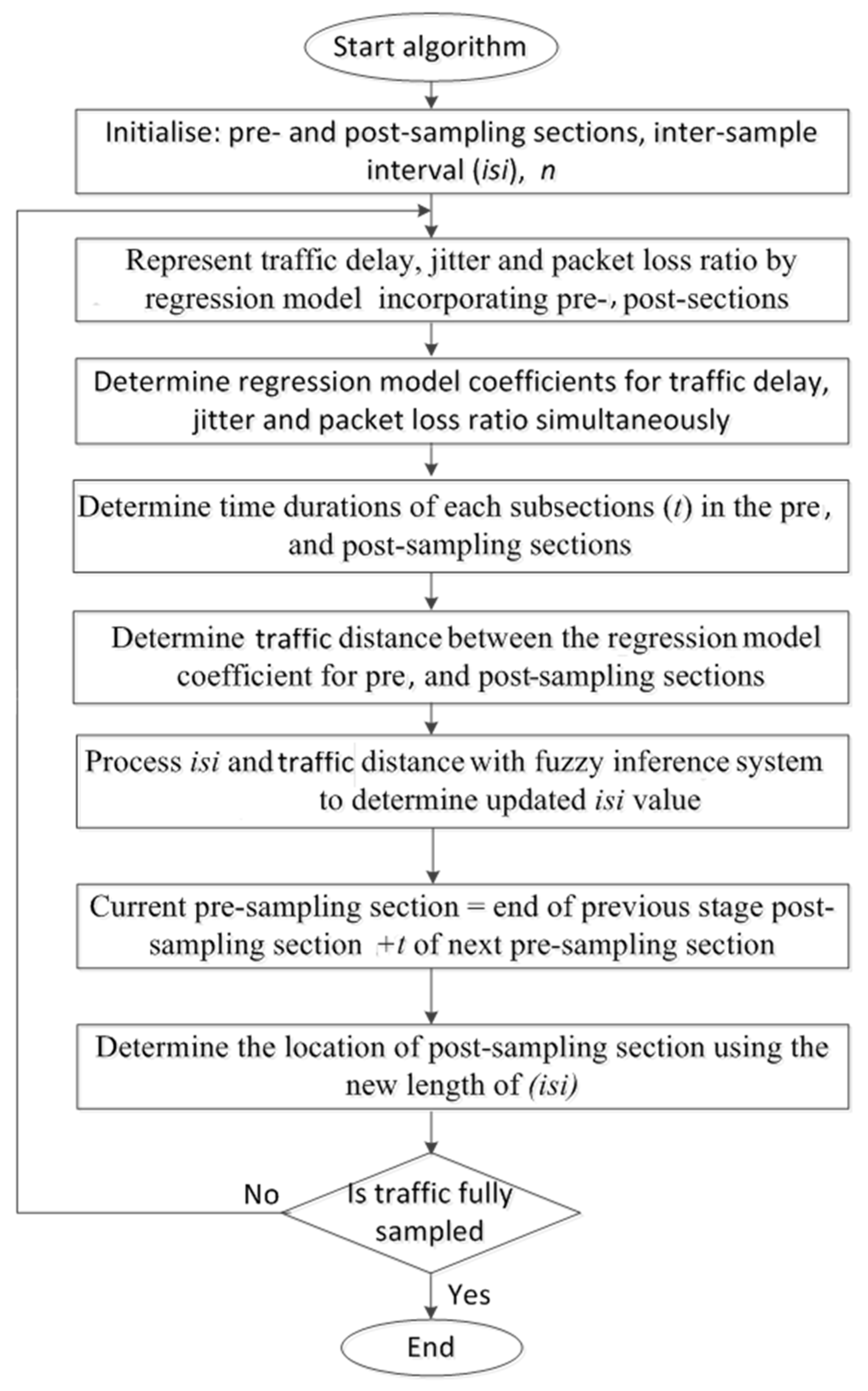
Once the traffic parameters (delay, jitter, and percentage packet loss ratio) were obtained, they were processed by the developed adaptive sampling method. The method used linear regression to model the traffic and the output from the model was interpreted by the fuzzy inference system (FIS) to dynamically adjust the number of packets selected for QoS assessment. The algorithm’s operation is illustrated in the flow chart shown in
Figure 4 and related diagram is shown in
Figure 5.
The elements of the algorithm are:
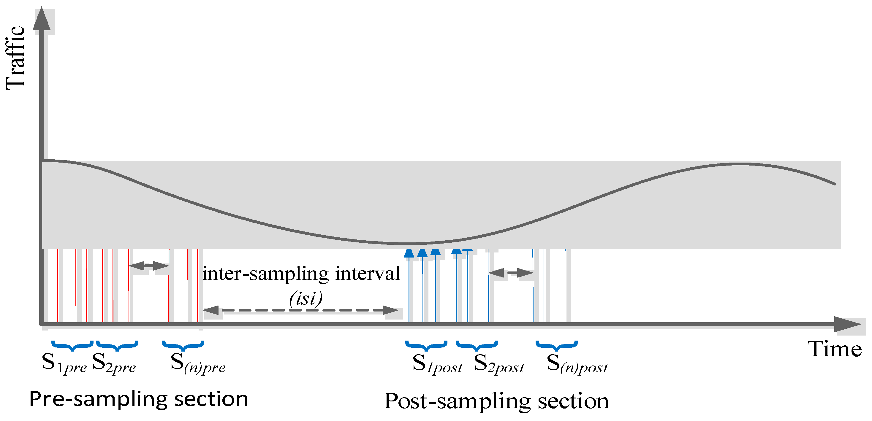
Pre- and post-sampling sections: These sections contain the traffic that needs to be sampled. The durations of these sections are kept fixed (predefined) and do not change during the sampling process.
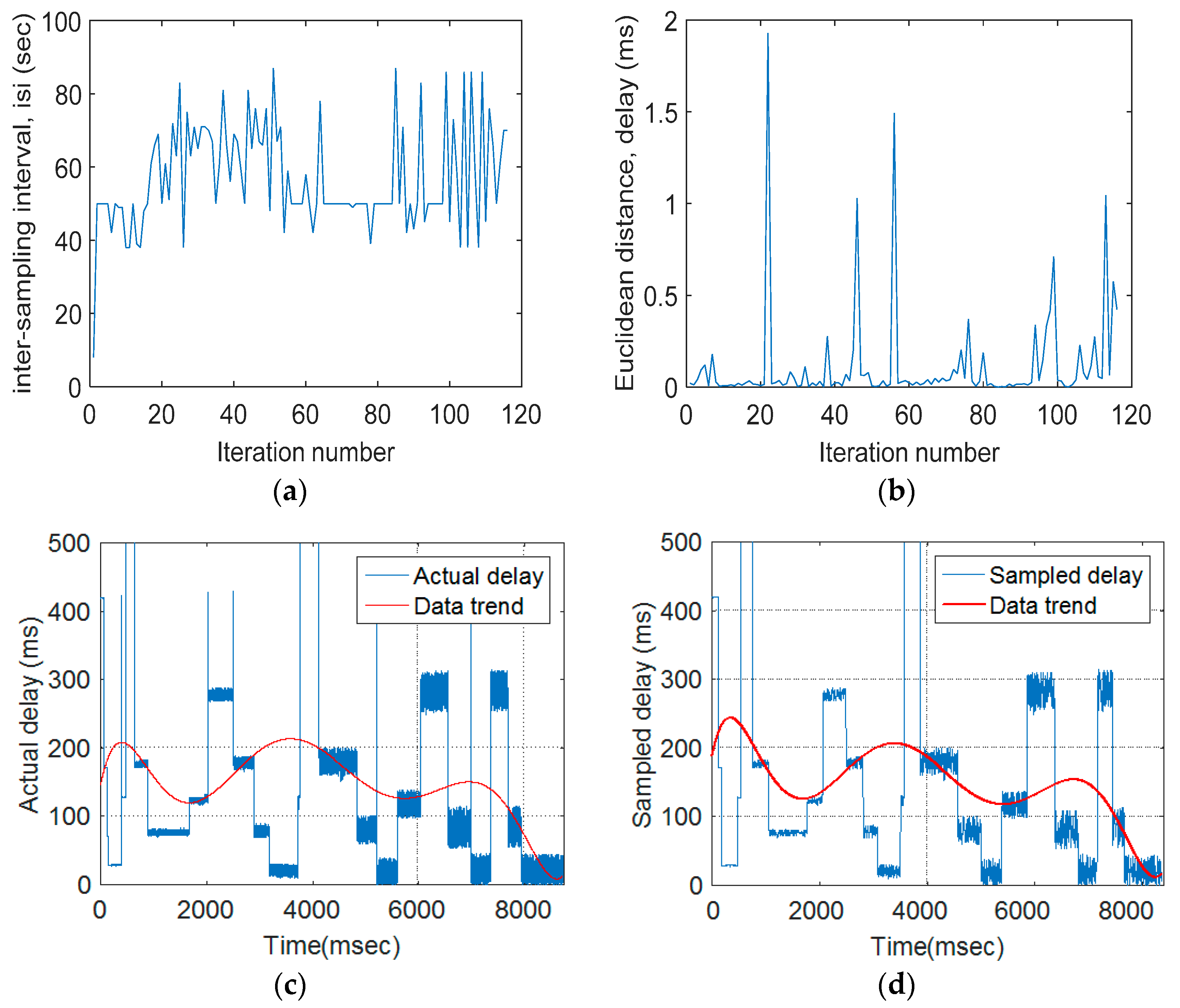
Inter-section interval (isi): This interval is between the pre- and post-sampling sections. Its duration is adaptively updated by the FIS.
Regression model: The traffic parameter (i.e., delay, jitter, and percentage packet loss ratio) were represented by an n × n matrix to allow regression analysis, where n is the number of subsections in the pre- and post-sampling sections. Each subsection contained n packets.
Euclidean distance (ED): ED was used to quantify the extent of traffic variations between the pre- and post-sampling sections.
Fuzzy inference system: FIS was used to update the duration of the isi based on its current value and the ED measures.
The regression model provided the traffic coefficients for the pre- and post-sampling sections. The traffic parameters delay, jitter, and percentage packet loss ratio were considered as the independent variables representing
p values in regression Equation (4). The pre- and post-sampling sections were divided into
n subsections (
s1,
s2, …,
sn), each subsection containing (
n − 1) packets as shown in
Figure 5; the traffic values of each subsection were represented by a row of matrix
P and the associated time period of every subsection was represented by the vector
T as indicated in Equation (4).
In this study,
n was chosen as 4, resulting in a 4 × 4 traffic matrix (
P). The matrix
P, depending on the type of analysis, represented delay values, jitter values, or percentage packet loss ratio values. This generated subsections S
1pre, S
2pre, S
3pre, and S
4pre for the pre-sampling section and S
1post, S
2post, S
3post, and S
4post for the post-sampling section. Each subsection contained 3 data packets. This was repeated for the pre- and post-sampling sections. The general representation of the traffic matrices for pre- and post-sampling sections is shown in Equation (4).
The time durations associated with each subsection (
s1,
s2, …,
sn) were represented by
t1,
t2, …,
tn. The vector
E = [
e1,
e2, …,
en] represents the measurement error, assumed to be zero in this study. These durations were measured by subtracting the arrival time of the last packet from the arrival time of first packet in the corresponding subsection. The regression coefficients
were determined by Equation (5).
The amount of variation in traffic associated with pre- and post-sampling sections was quantified by comparing their respective regression model coefficients using the Euclidean distance, as shown in Equation (6).
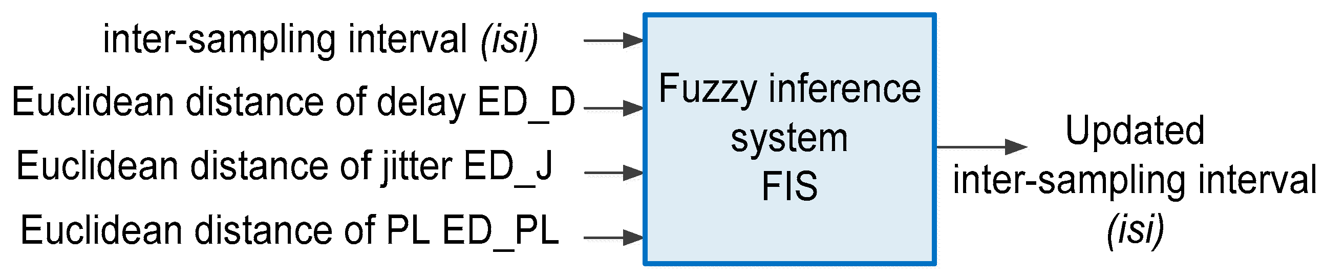
FIS received the current duration of the inter-sampling interval (
isi) and the Euclidean distance (
ED), and then determined the updated value of
isi duration as shown in
Figure 6.
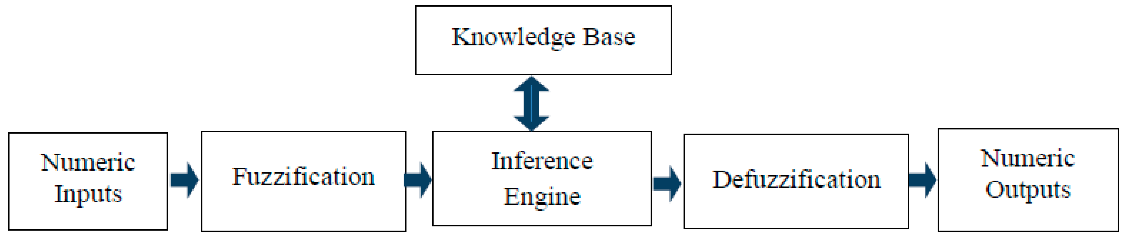
The Mamdani-type FIS was used to adaptively adjust the length of the
isi. Four inputs were fed into the FIS. They were the current inter-sampling interval, and the network parameters delay, jitter, and percentage packet loss ratio. The inputs and the output were fuzzified using the Gaussian membership functions that have a concise notation and are smooth. The Gaussian membership function is represented by the formula expressed in (7) where
ci and
σi are the mean and standard deviation of the
ith fuzzy set
Ai [
17].
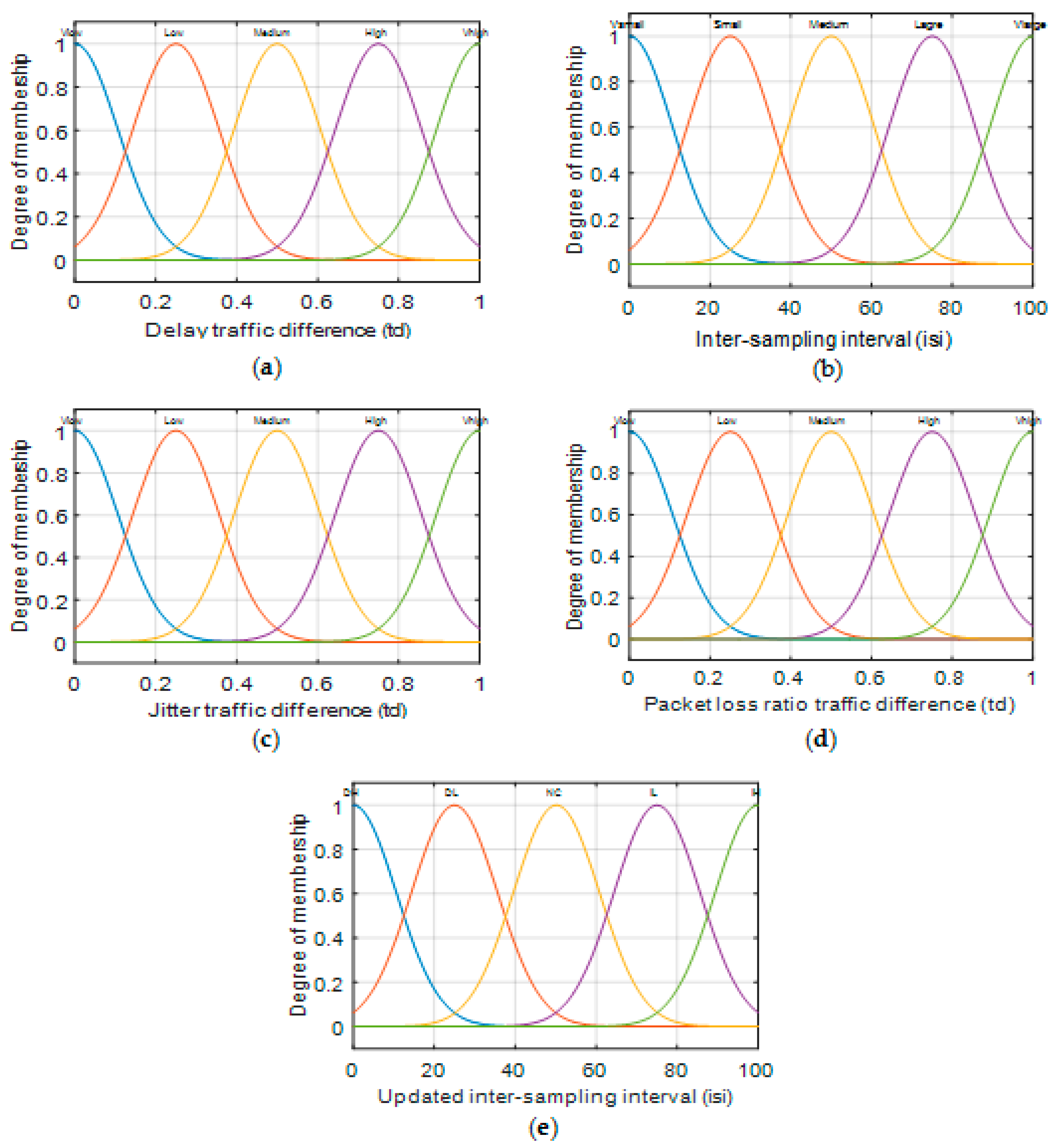
The inputs to the fuzzy inference system—the values of traffic Euclidean distance for delay, jitter, and percentage packet loss ratio, and the inter-sampling interval (
isi)—were individually fuzzified by five membership functions. The Euclidean distances for delay, jitter, and packet loss were represented by
VLow,
Medium,
High, and
VHigh fuzzy sets. The input inter-sampling interval (
isi) was represented by
VSmall, Small,
Medium,
Large, and
VLarge fuzzy sets. The output was defuzzified by four membership functions, represented by
IL (Low Increase),
NC (no change),
DL (Low Decrease), and
DH (High decrease). These membership functions are shown in
Figure 7.
Table 1 and
Table 2 show the mean and standard deviations of the Gaussian membership functions for the fuzzy input sets (i.e., delay, jitter, %PLR, and current
isi) and fuzzy output sets (i.e., updated
isi), respectively.
The relationship of the inputs, current
isi duration, and the Euclidean distance with the output (i.e., updated
isi duration) was represented by twenty rules, as shown in
Table 3.
The inputs to the FIS, i.e., the
ED and current inter-sample interval, were fuzzified using three membership functions. The
ED was represented by
Low,
Medium, and
High fuzzy sets and the current inter-sample interval (
isi) was represented by
Small,
Medium, and
Large fuzzy sets. The output was defuzzified by four membership functions, represented as
IL (low increase),
NC (no change),
DL (low decrease), and
DH (high decrease). These membership functions are shown in
Figure 7.
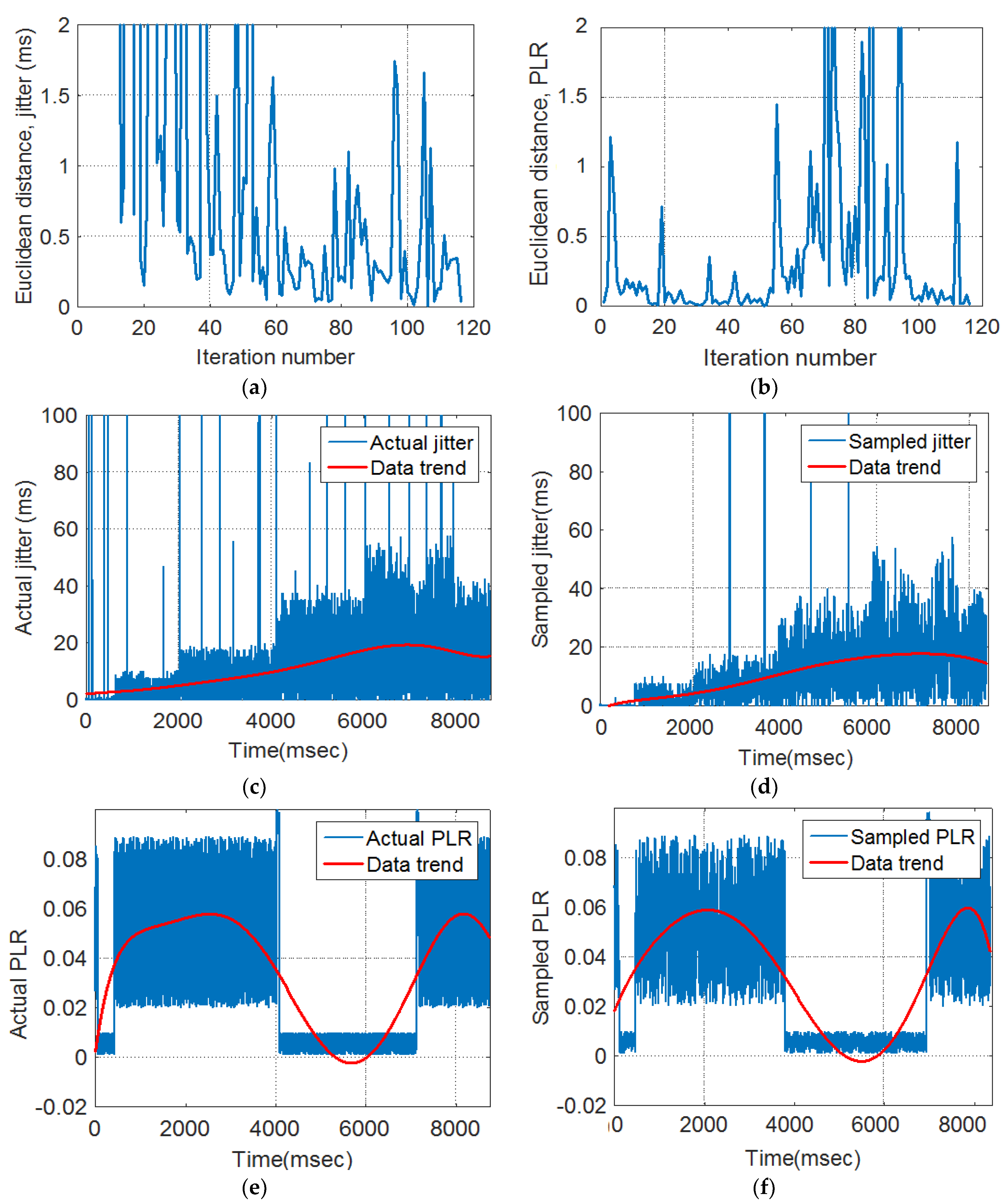
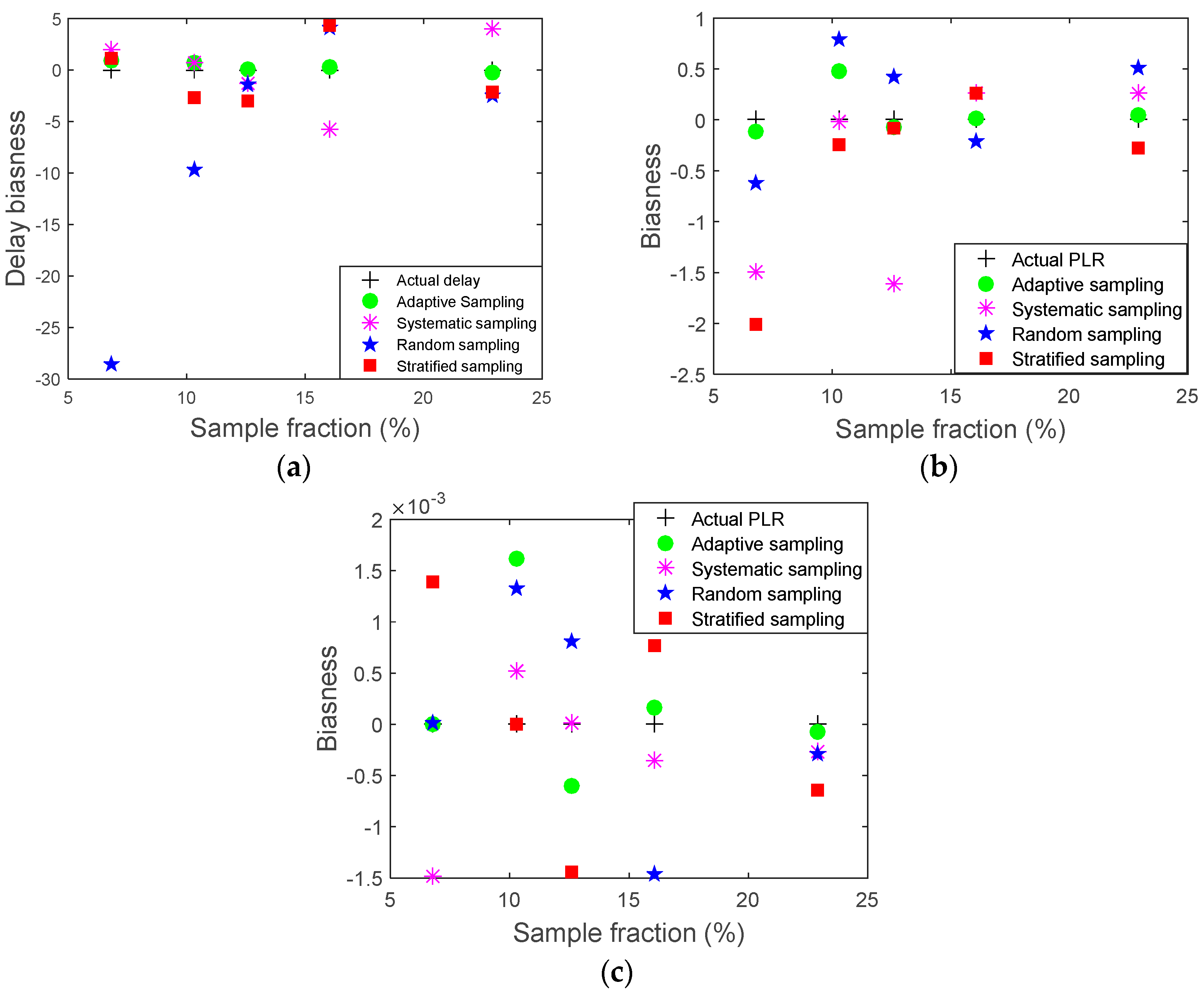
To evaluate the effectiveness of the developed adaptive sampling method, comparisons of the original traffic’s data packets and its sampled versions were carried out. Comparisons of mean and standard deviation of the sampled packets to those of its original populations may not be enough to evaluate the accuracy of the sampled version in terms of demonstrating the original population as they can be obscured by outliers [
30,
31]. Therefore, additional evaluations were used to assess the efficiency of the developed sampling approach. The bias indicates how far the mean of the sampled data lies from the mean of its original population [
31]. Bias is the average of difference of all samples of the same size. The bias was calculated as in Equation (10):
where
N is the number of simulation runs, and
Mi and
M are the means of the traffic parameters for the original data and its sampled population.
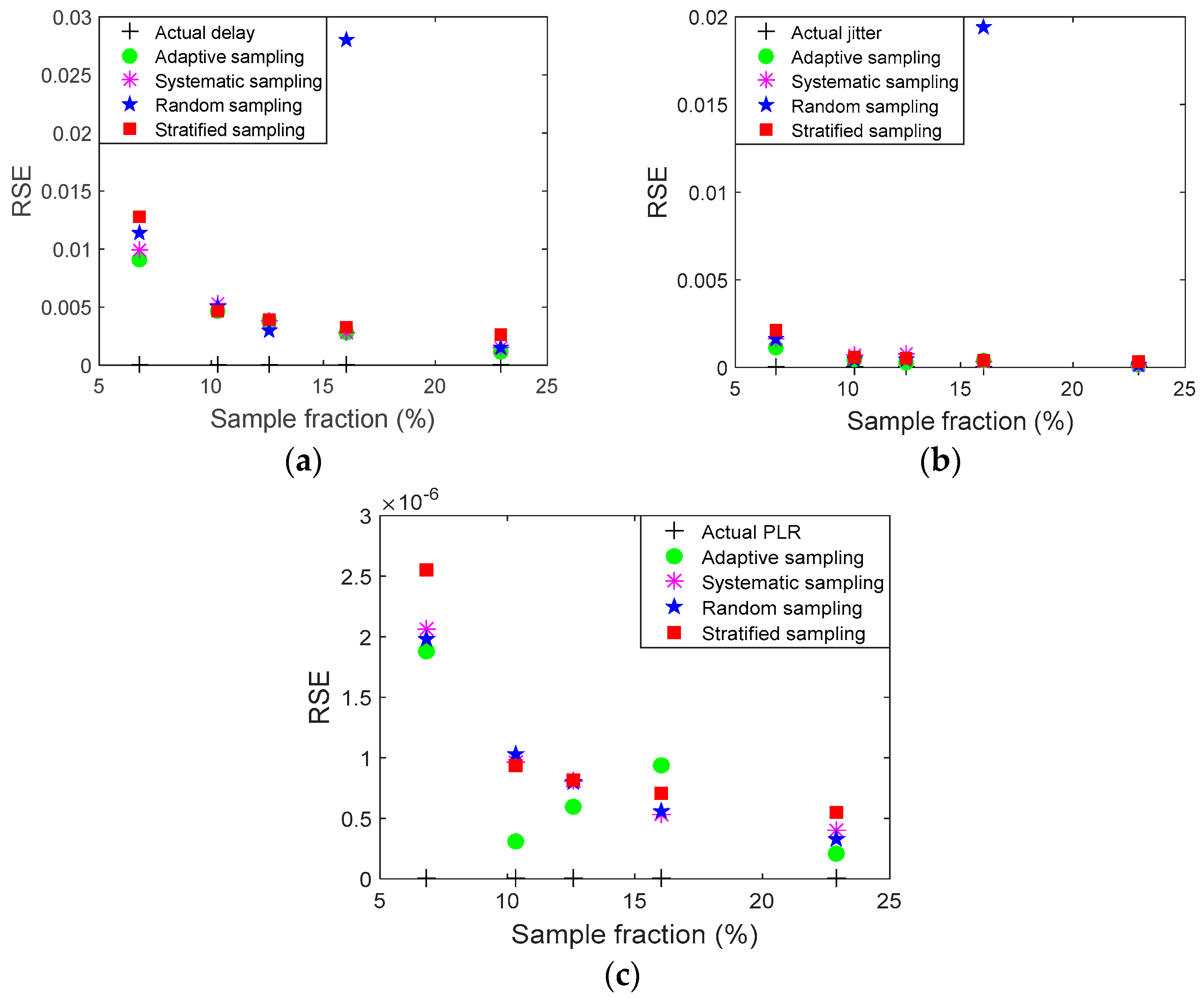
The Relative Standard Error (RSE) is another parameter that can be used to assess the accuracy and efficiency of the technique—RSE examines the reliability of sampling [
13]. RSE is defined as a percentage and can be defined as the standard error of the sample (SE) divided by the sample size (
n), as in Equation (11):
where
n is the sample size, and SE is the standard error values of the original and sampled data population.
Curve fitting is another measurement method that has been used to demonstrate the behaviour of the sampled data version in terms of representing the original data population. It examines the trends of the sampled data version and its equivalent original data by applying the curve fitting approach. Curve fitting is a suitable tool for representing a data set in linear, quadratic, or polynomial forms [
32] [
33]. Data curve fitting is based on two functions—the polynomial evaluation function and the polynomial curve fitting function. The general formula for a polynomial is shown in Equation (12).
The polynomial curve fitting function measures a least squares polynomial for a given data set of
x and generates the coefficients of the polynomial which can be used to illustrate a curve to fit the data according to the specified degree (
N). The degree of a polynomial is equal to the maximum value of the exponents (
N), and [
a0 …
aN] is a set of polynomial coefficients. The polynomial evaluation function examines a polynomial for
x values and then produces a curve to fit the data based on the coefficients that were found using the curve fitting function [
32,
33].
The sampling fraction is the proportion of a population that will be counted. Sampling fraction is the ratio of the sampled size (n) divided by the population size. In this study, the curve fitting results have been marked by a red color to demonstrate original and sampled data trends.


