Aerodynamic Modeling of NREL 5-MW Wind Turbine for Nonlinear Control System Design: A Case Study Based on Real-Time Nonlinear Receding Horizon Control

Abstract

The work presented in this paper has two major aspects: (i) investigation of a simple, yet efficient model of the NREL (National Renewable Energy Laboratory) 5-MW reference wind turbine; (ii) nonlinear control system development through a real-time nonlinear receding horizon control methodology with application to wind turbine control dynamics. In this paper, the results of our simple wind turbine model and a real-time nonlinear control system implementation are shown in comparison with conventional control methods. For this purpose, the wind turbine control problem is converted into an optimization problem and is directly solved by the nonlinear backwards sweep Riccati method to generate the control protocol, which results in a non-iterative algorithm. One main contribution of this paper is that we provide evidence through simulations, that such an advanced control strategy can be used for real-time control of wind turbine dynamics. Examples are provided to validate and demonstrate the effectiveness of the presented scheme.

1. Introduction

The overall objective of wind turbine control, in its simplest form, is mainly to maintain desired performance objectives (maximum power extraction, stability, etc.) during the process of wind energy utilization. However hefty the initial investment and maintenance costs will be, they will be offset by the fact that freely and naturally occurring wind power is being used in place of fuel [1]. In order to find a trade-off strategy between the load reduction and the power generation, a power curve is utilized to determine the best operation strategy. This work is based on the model of the NREL (National Renewable Energy Laboratory) 5-MW reference wind turbine for nonlinear control system development. In addition, in later sections, we will show that dynamic models of the turbine are used to design controls and to simulate the behavior of the system.

In control methodologies, the models of wind turbines range from low-fidelity to medium-fidelity models. The low-fidelity models consist of reduced order models utilized for control design. They consider only the most expressive modes of the dynamics (rotational movement of the rotor and pitch movement of the floating platform, when applicable) and provide a valuable insight into the problem. The medium-fidelity models are usually utilized for the simulation of the low-fidelity models and certification of the turbine under extreme events [1]. An example of a medium-fidelity simulator is the NREL FAST (Fatigue, Aerodynamics, Structures and Turbulence), which simulates 18 modes (plus six if simulating offshore turbines) [2]. In this paper, we concentrate our efforts on the development of low-fidelity models that are still accurate and reliable and those that satisfy high precision and performance characteristics.

The highest-fidelity turbine modeling option usually comes with a combination of a Computational Fluid Dynamics (CFD) code, a detailed fluid-structure interaction model and a finite element code. This level of fidelity comes with the cost of heavy computational requirements and is not utilized in this paper.

On the other hand, nonlinear control system design and analysis of wind turbine dynamics has become an important research topic in recent years. There are many valuable studies in the literature concentrating on the nonlinear control of wind turbine dynamics. One of the notable works belongs to Song et al. (2000), where they concentrated their efforts on the variable speed control of wind turbines using nonlinear and adaptive algorithms [3]. Boukhezzar et al. (2009) investigated nonlinear control with wind estimation of a variable speed wind turbine [4]. In another recent study of Boukhezzar (2011), attention was given to the nonlinear control of a variable-speed wind turbine using a two-mass model [5]. Beltran et al. (2008) took the sliding mode control approach for the variable speed energy conversion systems [6]. Wu et al. (2008) studied the decentralized nonlinear control dynamics of a wind turbine [7]. An interesting approach was taken by Schlipf (2013) to analyze wind turbine dynamics through nonlinear model predictive control using Light Imaging, Detection, And Ranging (LIDAR) measurements [8], where the authors provide some preliminary results on a nonlinear receding horizon control application on wind turbine dynamics as reported in Galvani et al. (2016) [9].

As a topic of interest, receding horizon control (RHC) [10,11] is a branch of model predictive control methodologies that aims to obtain an optimal feedback control law by minimizing the given performance index. The performance index of a receding-horizon control problem has a moving initial time and a moving terminal time, where the time interval of the performance index is finite. Since the time interval of the performance index is finite, the optimal feedback law can be determined even for a system that is not stabilizable. The receding horizon optimal control technique can handle a broader class of control objectives than asymptotic stabilization [12]. The receding horizon control was originally applied to linear systems and then was extended to nonlinear systems [13,14,15,16]. Through its functionality, nonlinear receding horizon control (NRHC) [15,16] has made an important impact on industrial control applications and is being increasingly applied in process controls. Various advantages are known for NRHC, including the ability to handle time-varying and nonlinear systems, input/output constraints, associated plant uncertainties, and so on.

In this study complementary to existing studies. we developed an improved wind turbine model which provides nonlinear real-time control approach for wind turbine dynamics based on the receding horizon control methodology focused on controlling rotor angular velocity. In this control methodology, we implement a solution scheme of real-time nonlinear control effort, which is independent of iterative solutions and constitutes the novel implementation suggested through this work. In addition, we demonstrate the applicability of such a real-time nonlinear receding horizon control methodology not only on onshore wind turbines, but also the effectiveness of such an application.

The paper is organized as follows: In Section 2, modeling of wind turbine dynamics is introduced, while in Section 3, the design overview is investigated. In Section 4, we provide the real-time nonlinear receding horizon control implementation on wind turbine dynamics, and with Section 5, we conclude the paper.

2. Modeling

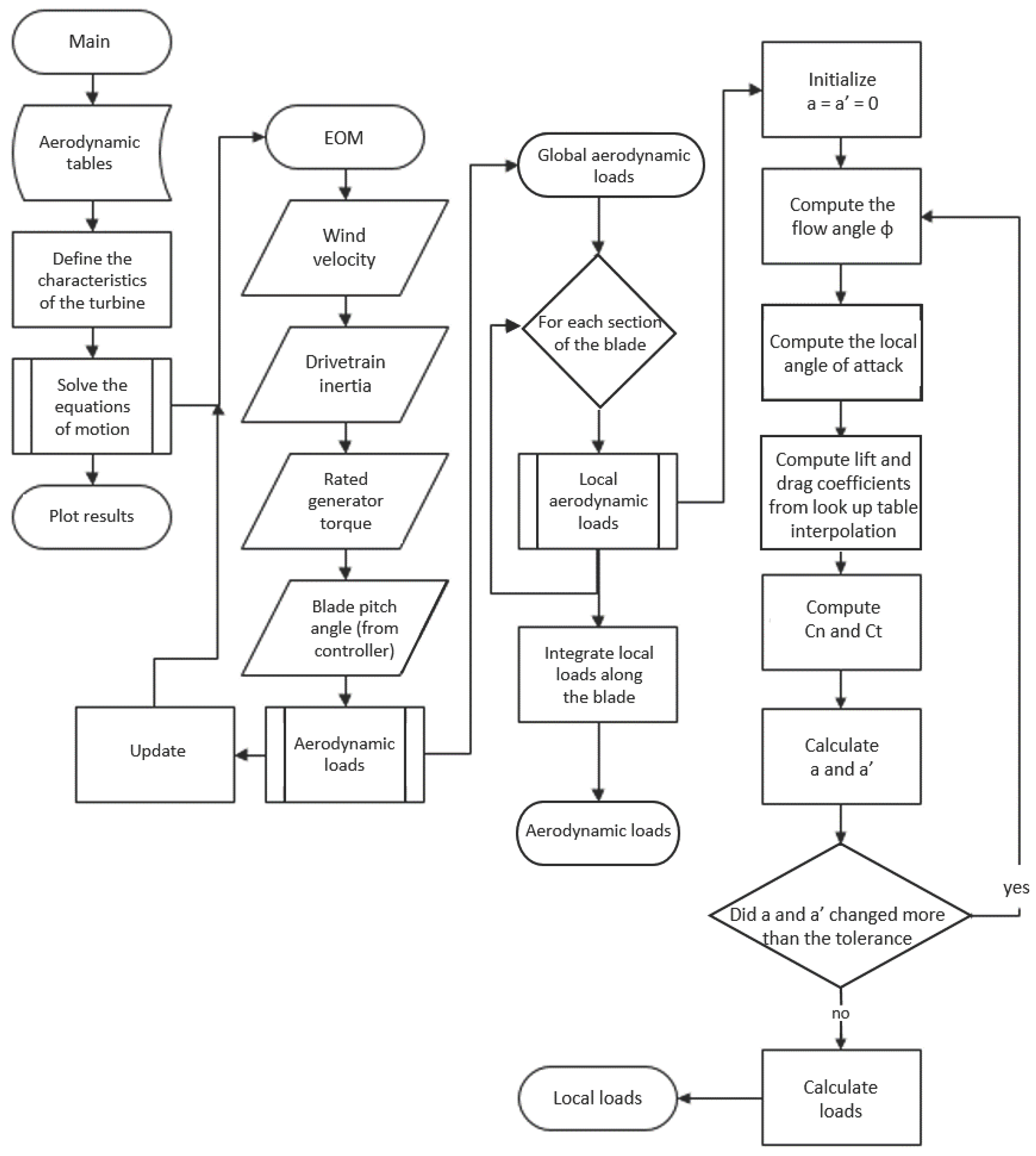
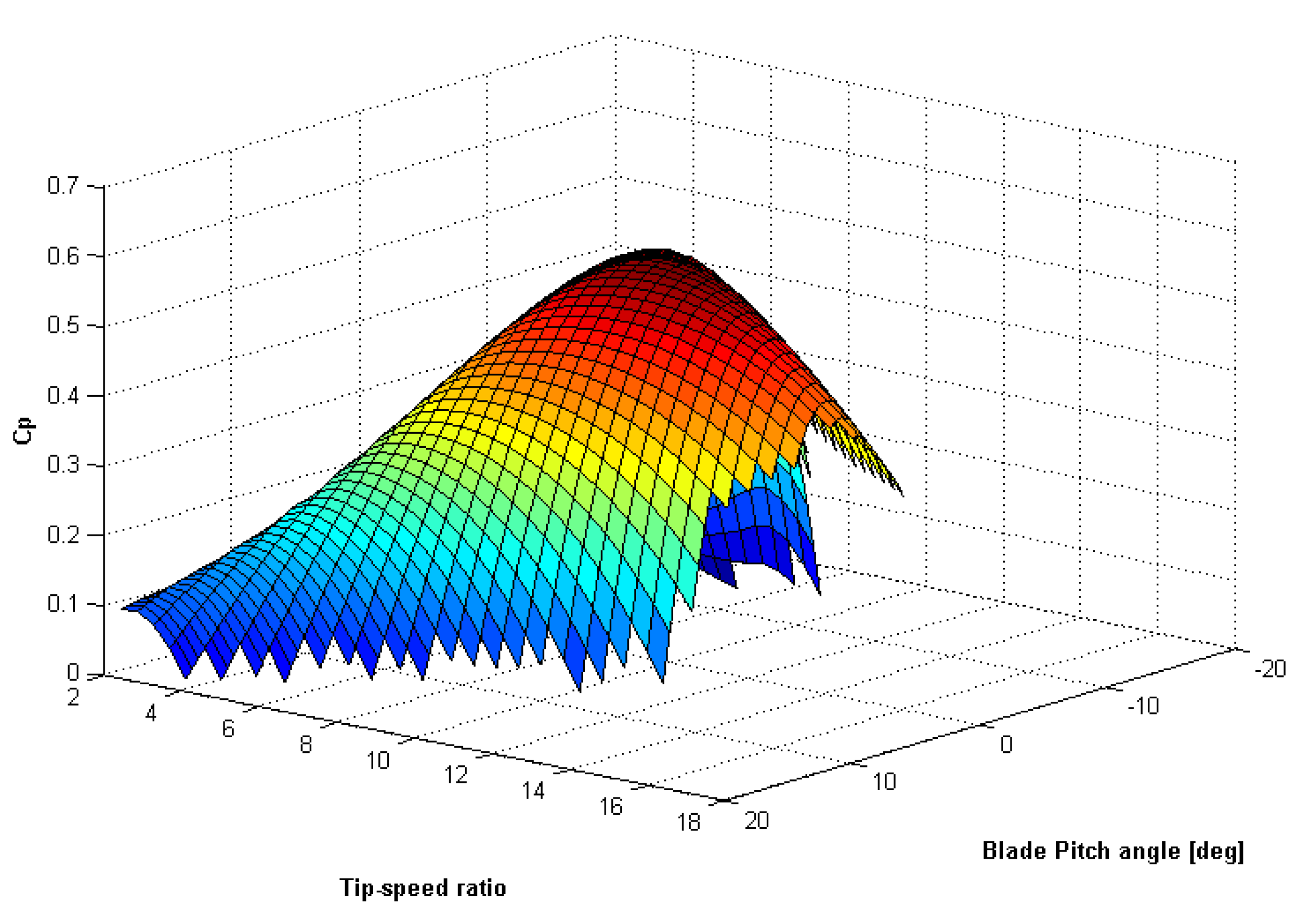
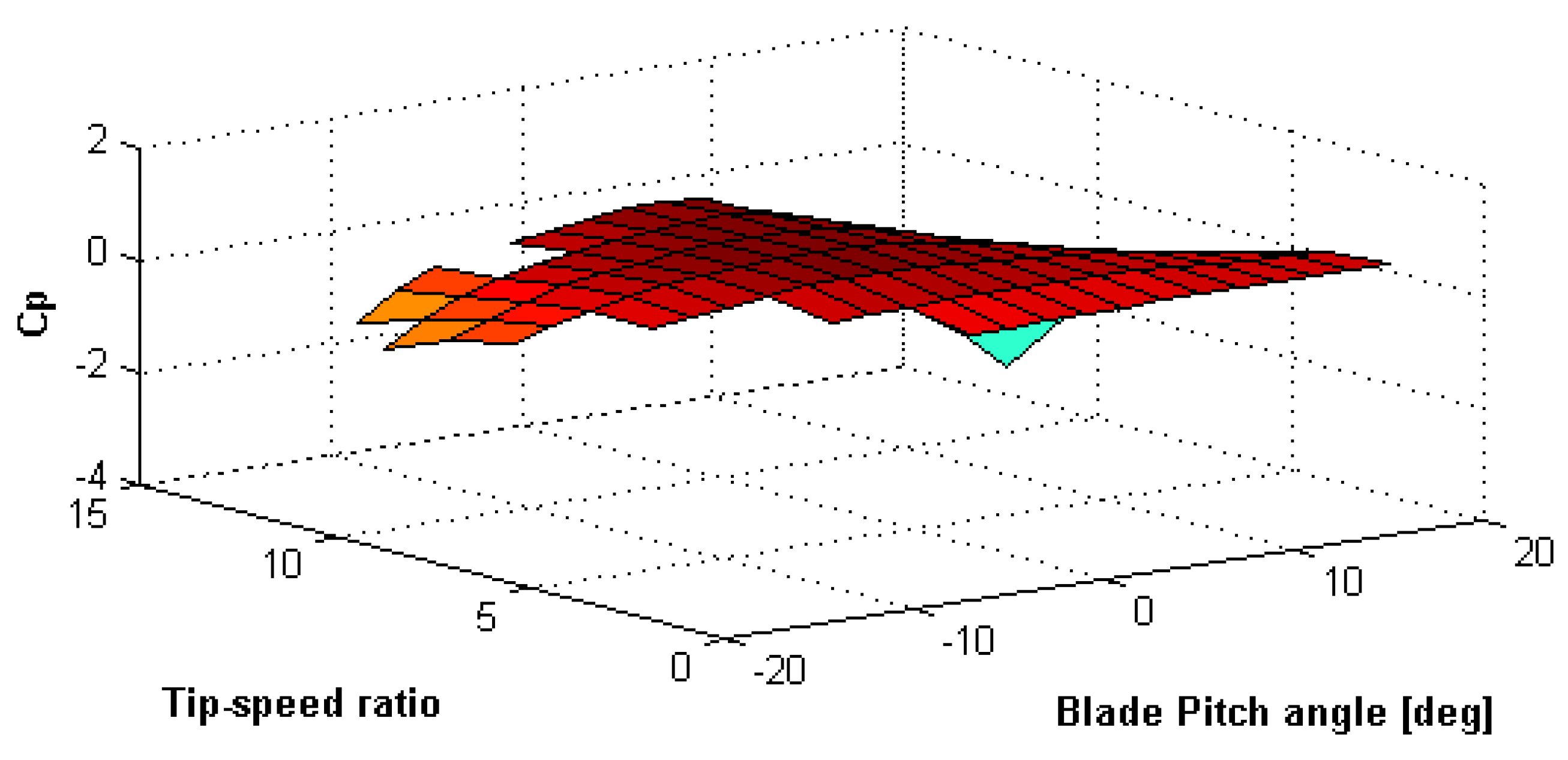
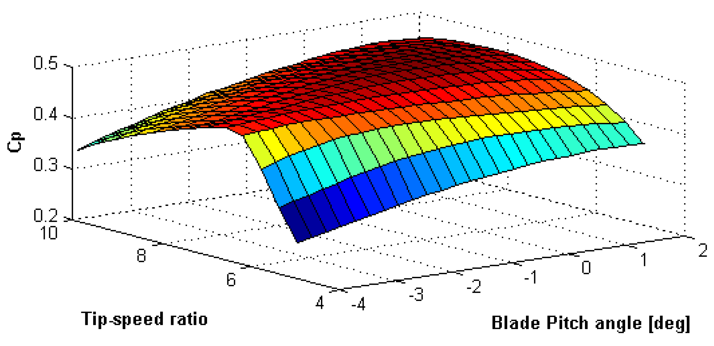
2.1. Aerodynamic Modeling

In this study, the NREL (National Renewable Energy Laboratory) 5-MW reference wind turbine dynamics is utilized for analysis and we provide the backbone of the modeling of a simple wind turbine model, which eventually is used in control system analysis (and design).

From a practical point of view, in order to simulate the dynamics of the turbine, the aerodynamic loads on the rotor must be calculated. Based on the 1D momentum theory and the blade element theory [17], a MATLAB code was developed to calculate the aerodynamic loads as a function of the pitch angle, rotor shaft rotational speed and wind conditions. The code was divided into two parts: the first part is responsible for calculating the local loads of each section of the blade, while in the second portion of the code, the overall disk momentum and normal loads are calculated through the integration of the local loads. This methodology is well defined in Hansen (2008) [18], and the aerodynamic characteristics (such as blade configuration and airfoil data) are available in Butterfield (2009) [19].

2.1.1. Local Loads Definition

Different from an aircraft wing, the angle of attack in wind turbines varies substantially along the blade. The variation comes from the fact that the tangential component of the wind velocity $\omega r(1+a^{\prime })$ is dependent on the distance from the root-r. For this reason, the aerodynamic curves of each section must be determined for the entire domain of the angles of attack.

Based on well known text-book information (as provided in Hansen (2008) [18], Fischer (2013) [20] and Jonkman (2007) [21]), the angle of attack is obtained using Equation (1).

$$\alpha =\varphi -\theta$$

(1)

where θ is the local pitch angle (which can be calculated by $\theta ={\theta }_b+\beta$), ${\theta }_b$ is the blade pitch angle and β is the twist angle of the section, respectively. Furthermore, ϕ could be obtained from:

$$tan(\varphi )=\frac{(1-a)V_0}{(1+a^{\prime })\omega r}$$

(2)

where a is the axial induction factor, $a^{\prime }$ is the tangential induction factor, $V_0$ is the wind speed, r is the distance between the section and the root of the blade and ω is the angular velocity of the rotor.

By the initialization of the induction factors, it is also possible to calculate the aerodynamic coefficients $C_n$ and $C_t$, accordingly.

$$C_n=C_{l}cos(\varphi )+C_{d}sin(\varphi )$$

(3)

$$C_t=C_{l}sin(\varphi )-C_{d}cos(\varphi )$$

(4)

Furthermore, the following relations can be derived:

$$V_{rel}sin(\varphi )=(1-a)V_0$$

(5)

$$V_{rel}cos(\varphi )=(1+a^{\prime })\omega r$$

(6)

After some algebra, the induction factors a and $a^{\prime }$ can be calculated as:

$$a=\frac{1}{\frac{4Fsi{n}^2(\varphi )}{\sigma C_n}+1}$$

(7)

$$a^{\prime }=\frac{1}{\frac{4Fsin(\varphi )cos(\varphi )}{\sigma C_t}-1}$$

(8)

where σ is the rotor solidity, given by:

$$\sigma =\frac{cB}{2\pi r}$$

(9)

Here, B represents the number of blades, and c is the chord of the section.

Prandtl’s tip loss factor and the Glauert correction for high values of axial induction factor were also implemented in the code. Prandtl’s tip loss factor is given by:

$$F=\frac{2}{\pi }co{s}^{-1}(e^{-f})$$

(10)

where:

$$f=\frac{B}{2}\frac{R-r}{sin(\varphi )r}$$

(11)

According to the Glauert correction, for $a>0.2$, it can be calculated by:

$$a=\frac{1}{2}(2+k(1-2.02)-\sqrt{{(k(1-2.02)+2)}^2+4(k0.2^2-1)})$$

(12)

where:

$$k=\frac{4Fsi{n}^2(\varphi )}{\sigma C_n}$$

(13)

By iterating the values of a and $a^{\prime }$ until convergence, the final values of the coefficients $C_n$ and $C_t$ can be calculated, numerically from Equations (3) and (4).

2.1.2. Global Loads Definition

After the calculation of the local loads for each segment of the blade, the rotor aerodynamic induced torque and the forces normal to the rotor are determined.

First, the local aerodynamic forces are calculated from the coefficients:

$$P_n=\frac{1}{2}\rho V_{rel}^{2}c{C}_n$$

(14)

$$P_t=\frac{1}{2}\rho V_{rel}^{2}c{C}_t$$

(15)

and then, using numerical integration:

$$T_{rotor}=B\int dM=B\int r{P}_{t}dr$$

(16)

$$F_{th}=B\int P_{n}dr$$

(17)

could be calculated with ease. Here, $T_{rotor}$ defines the rotor torque, and $F_{th}$ presents the overall force applied normal to the rotor (thrust).

In this specific study, each blade is divided into 100 (hundred) sections where the convergence criteria (tolerance) are set up as 0.01, between the iterations. On an Intel core i7 laptop computer, the aerodynamic load computations (including reading from the data files) take approximately 7–10 s.

2.2. Equations of Motion

When considering control purposes, the equations of motion can be separated into two segments, onshore turbines and offshore turbines.

2.2.1. Onshore Wind Turbines

Considering that the tower and blades’ elasticity are neglected, we have an one-state, rigid body model of the turbine rotor. Therefore, from Newton’s law:

$$\dot{\omega }=\frac{1}{I_d}(T_{rotor}-T_{gen})$$

(18)

could be defined, where $T_{gen}$ is the generator torque and $I_d$ is the drive-train inertia, which includes the inertia of the rotor, generator and transmission.

Figure 1 summarizes the procedure implemented to simulate and analyze the onshore turbine. Being highly dependent on the wind velocity and rotational velocity of the rotor, we can observe that most of the code is dedicated to updating the aerodynamic loads.

It is important to note that the presented simplistic wind turbine model dynamics is not a transient model. Therefore, it does not include the effects of the rotational and tilt dynamics, yaw motion and pitching motion, as well as the complex motions for offshore turbines. With this said, the aim and intention with the model is to obtain a simple, yet accurate rotational speed dynamics architecture that could be used for more advanced and sophisticated revolutions per minute (RPM) control purposes.

In addition, it is worth emphasizing that the presented wind turbine model dynamics is not taking into consideration the designed tilt/precone angle of the NREL 5-MW turbine dynamics and concentrates on the general dynamics of the wind turbine with emphasis on the RPM control architecture.

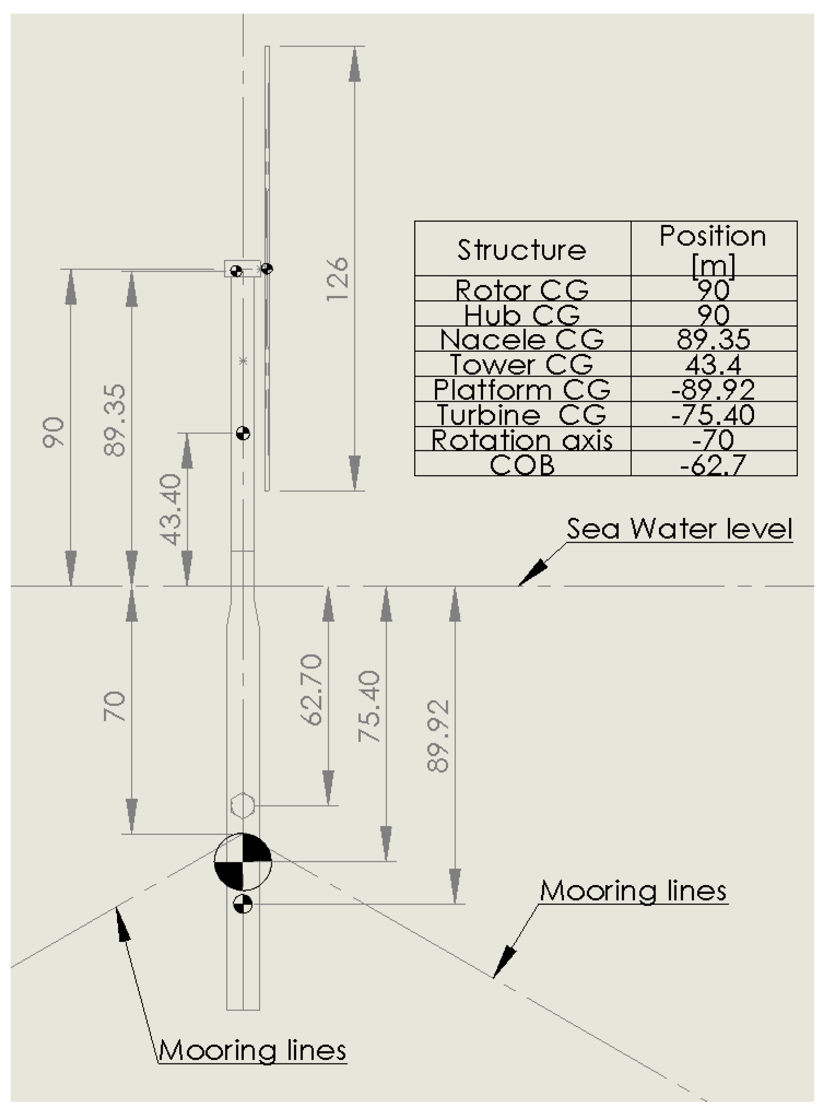
2.2.2. Offshore Wind Turbines

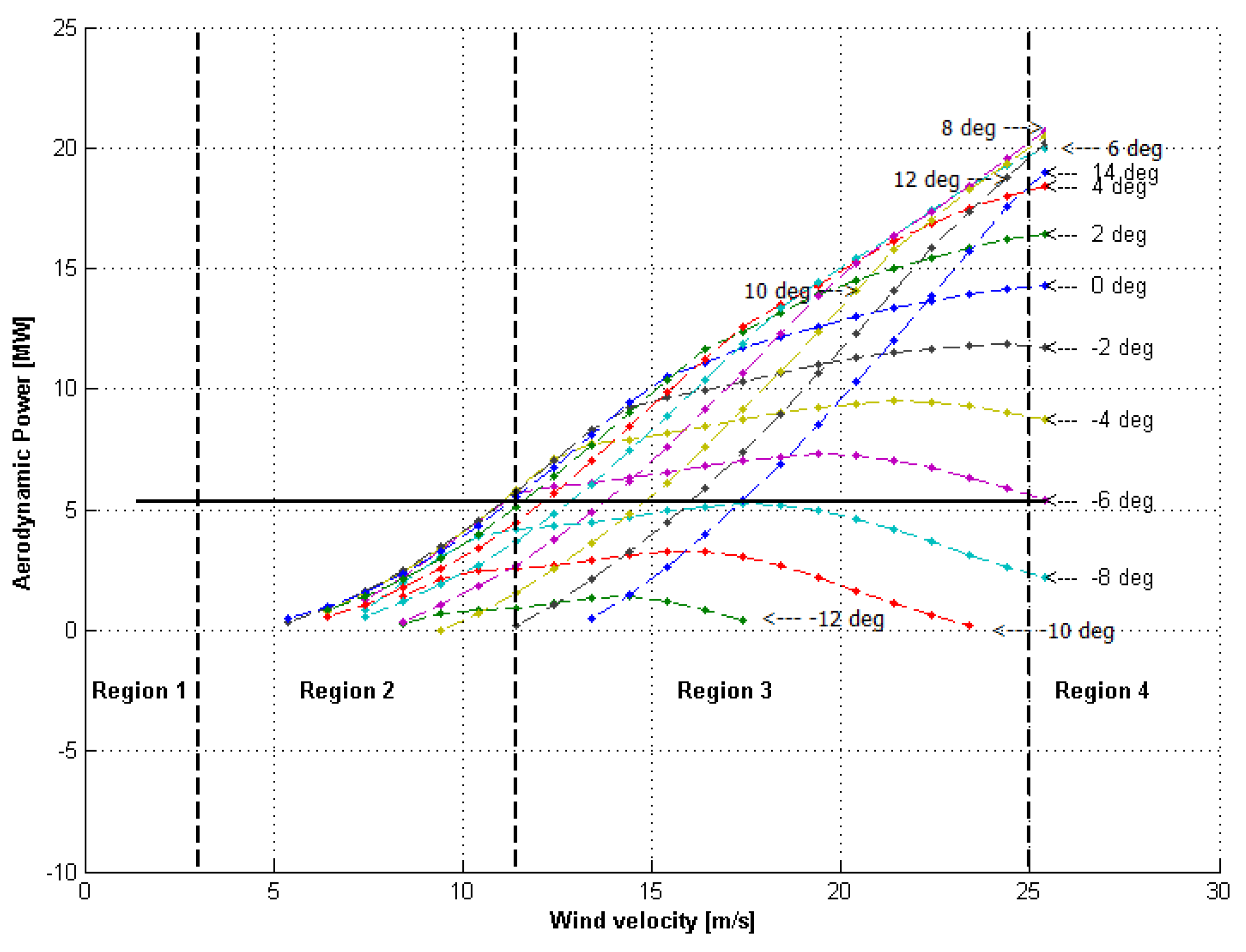
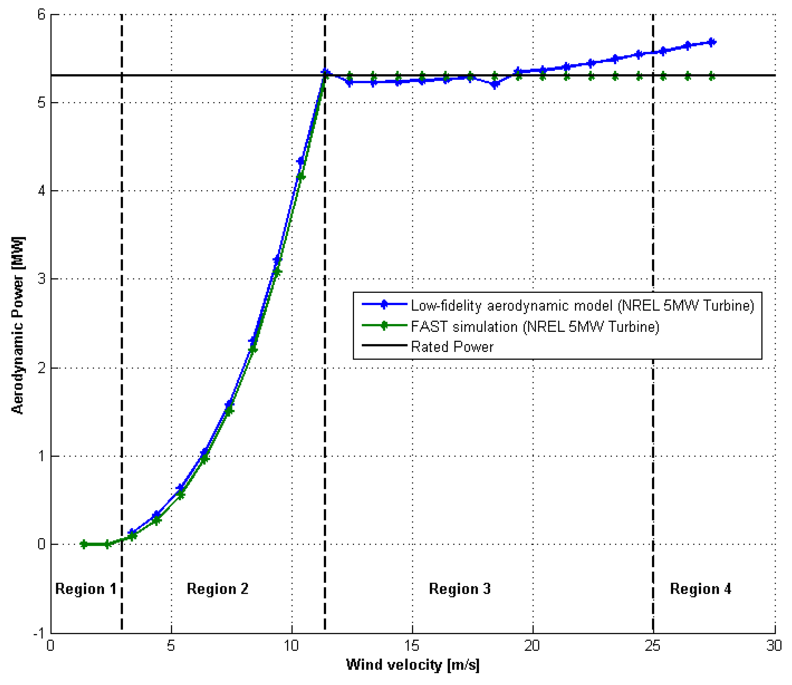
Modeling offshore wind turbines requires the consideration of at least one more degrees of freedom (DOF). Generally speaking, when mounted on a floating platform, the pitch movement of the turbine-platform (different from blade pitch angle) changes the overall wind velocity that the rotor experiences. This induced variation in the wind velocity may cause instability. Figure 2 shows a schematic of the NREL 5-MW wind turbine mounted on the OC3-Hywind spar buoy platform.

Therefore, the model includes Equation (18) and the following equation:

$$J_T\ddot{\varphi }+D_T\dot{\varphi }+C_T\varphi =L_T{F}_{th}$$

(19)

where ϕ is the turbine pitch angle, $J_T$ is the moment of inertia of the system with respect to the center of oscillation (for hydrodynamic systems, the consideration of the added mass is required), $D_T$ is hydrodynamic damping, $C_T$ is the hydrodynamic stiffness, $L_T$ is the distance between the rotor shaft and the center of oscillation and $F_{th}$ is the aerodynamic force normal to the rotor.

Ideally, the goal will be to extend the study to offshore wind turbines, but currently, this is an ongoing research topic and is not included within the study. Obtained results will be presented in another study.

2.2.3. Power Curve

The operation of the turbine is determined by the aerodynamic power curve, as shown in Figure 3 and Figure 4. Figure 3 was extracted from the aerodynamic model, developed above, and represents the power extracted from the wind for different wind velocities and different collective blade pitch angles (the rotational speed of the rotor was considered the rated rotational speed of the 5-MW reference turbine). In Region 1, the turbine does not operate due insufficient winds. By analyzing Region 2 of the plot, we can identify the pitch angle that would provide the higher power extraction $\overline{\theta }$. $\overline{\theta }$ is called the fine pitch angle. Its analysis is developed in Section 3.1 and shown in [19]. The fine pitch angle for the turbine is 0.0^o. By analyzing Region 3, we can see that the rotor is able to extract more power from the wind than its maximum extraction. However, operating above the rated power would induce excessive loads on the structure, compromising the life cycle of the turbine. In Region 4, the turbine is shut down to avoid structural damage.

Figure 4 was obtained by extracting the rotational speed of the rotor ω, the rotor torque $T_{rotor}$ and the blade pitch angle θ from FAST, for different wind velocities. Because FAST simulates in the time domain and has a controller already implemented, the values were obtained after the turbine settled. Then, ω, θ and the wind velocity were inputted into the aerodynamic model. Therefore, Figure 4 represents a comparison of the low-fidelity aerodynamic model and the medium-fidelity FAST model, along the operation curve.

Additionally, the controlled version of the power curve is shown in Figure 5.

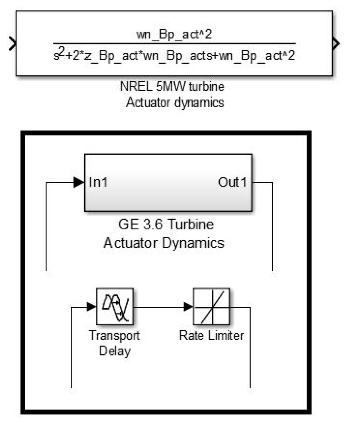
2.2.4. Actuator Dynamics

According to Butterfield (2009) [19], FAST model dynamics do not include a blade-pitch actuator dynamic effect. Therefore, an actuator dynamics with a natural frequency of 30 Hz and damping ratio of 2% was suggested for further simulations.

On the other hand, Miller (2003) [22] suggests a simpler approach for the General Electric (GE) 3.6-MW turbine dynamics, where the actuator is simulated by constraining the blade pitch angle rate and delaying the control signal. Both approaches were implemented in the Simulink environment for this study. Figure 6 shows the second order transfer function for the NREL approach and the block for the GE approach.

3. Control Analysis and Design Overview

The operation of the turbine relies on two basic controls: the generator-torque controller in Region 2 and the rotor-collective blade-pitch angle control in Region 3. The goal of the generator-torque controller is to maximize the power capture while the goal of the blade-pitch controller is to regulate the rotational speed of the generator/rotor. In addition, there are also different control loops to stop the turbine and yaw control to direct the turbine along the wind direction.

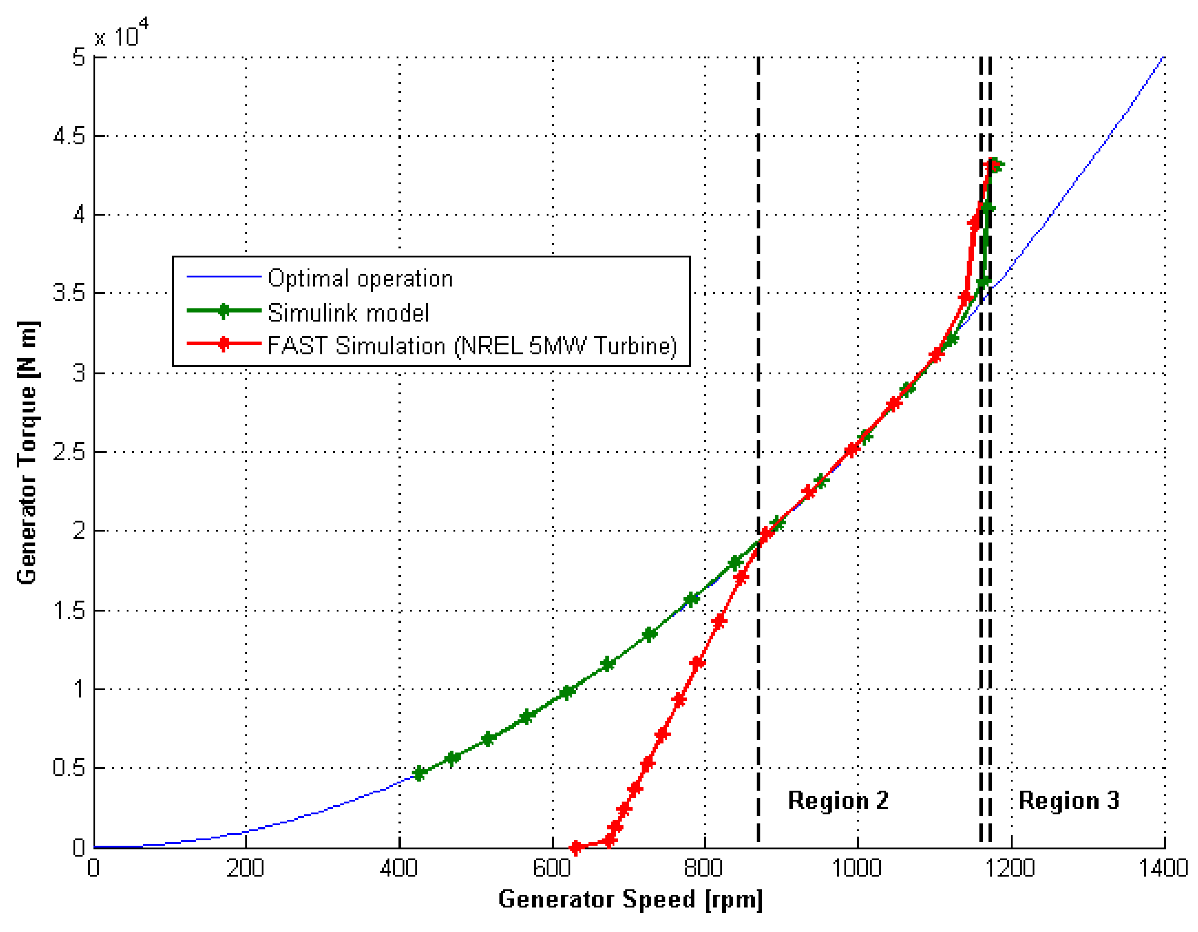
3.1. Generator-Toque Control

3.1.1. Formulation

The goal of Region 2 control is to maximize the energy capture. As stated in Ozdemir (2013) [1], a typical Region 2 controller could be defined as:

$$T_{gen}=K{\omega }_r^2$$

(20)

$${\theta }_i=\overline{\theta }$$

(21)

where ${\theta }_i$ is the input blade pitch angle, K is the proportional gain and ${\omega }_r$ is the rotor angular speed. Johnson (2004) [23] provides a methodology to calculate the gain K as:

$$K=\frac{1}{2}\rho A{R}^3\frac{C_{p_{max}}}{{\lambda }_{*}^3}$$

(22)

where ρ is the air density, A is the rotor area, R is the blade length, ${\lambda }_{*}$ is the tip-speed ratio related with $C_{p_{max}}$ and $C_{p_{max}}$ is the maximum power coefficient. The tip-speed ratio (TSR) is defined by:

$${\lambda }_{*}=\frac{\omega R}{V_0}$$

(23)

and $C_p$ is defined by:

$$C_p=\frac{P}{P_{wind}}$$

(24)

where P is the rotor aerodynamic power and $P_{wind}$ is the wind power, given by:

$$P_{wind}=\frac{1}{2}\rho A{V}_0^3$$

(25)

Using Equation (20), the generator torque is controlled to track the optimal generation curve, as shown in Figure 7. In the wind turbine industry, the generators are generally used as induction generators, which allow the control of the torque. Therefore, the control law is intended to keep the turbine operating at the peak of its Cp-TSR-pitch surface [23].

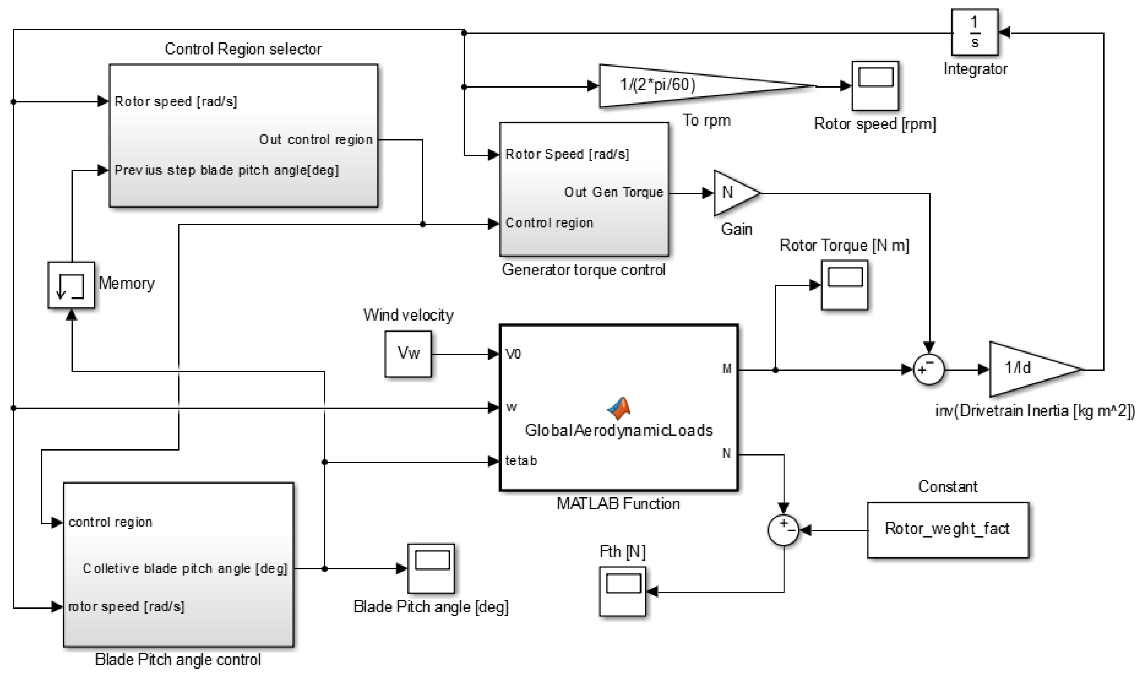
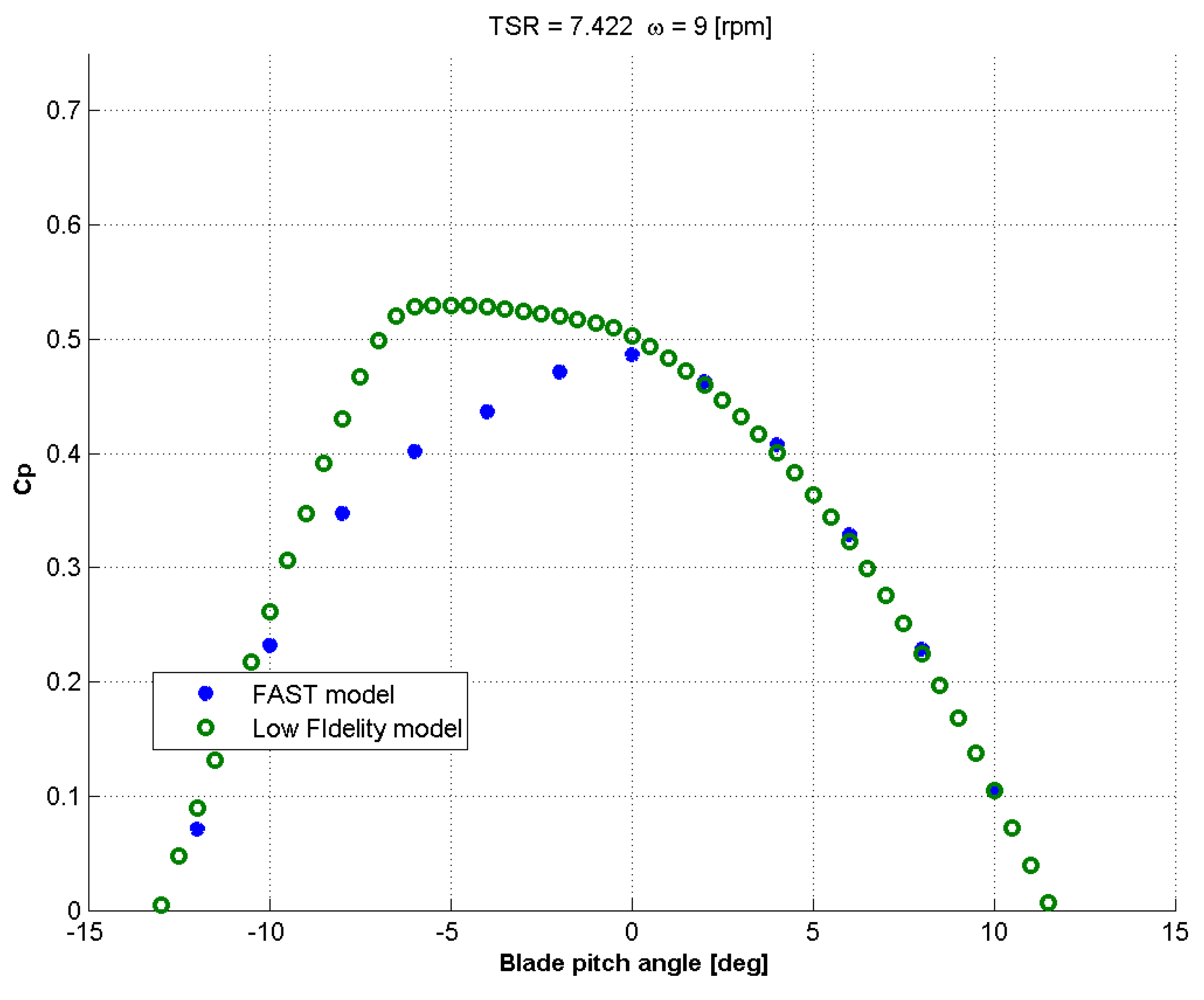
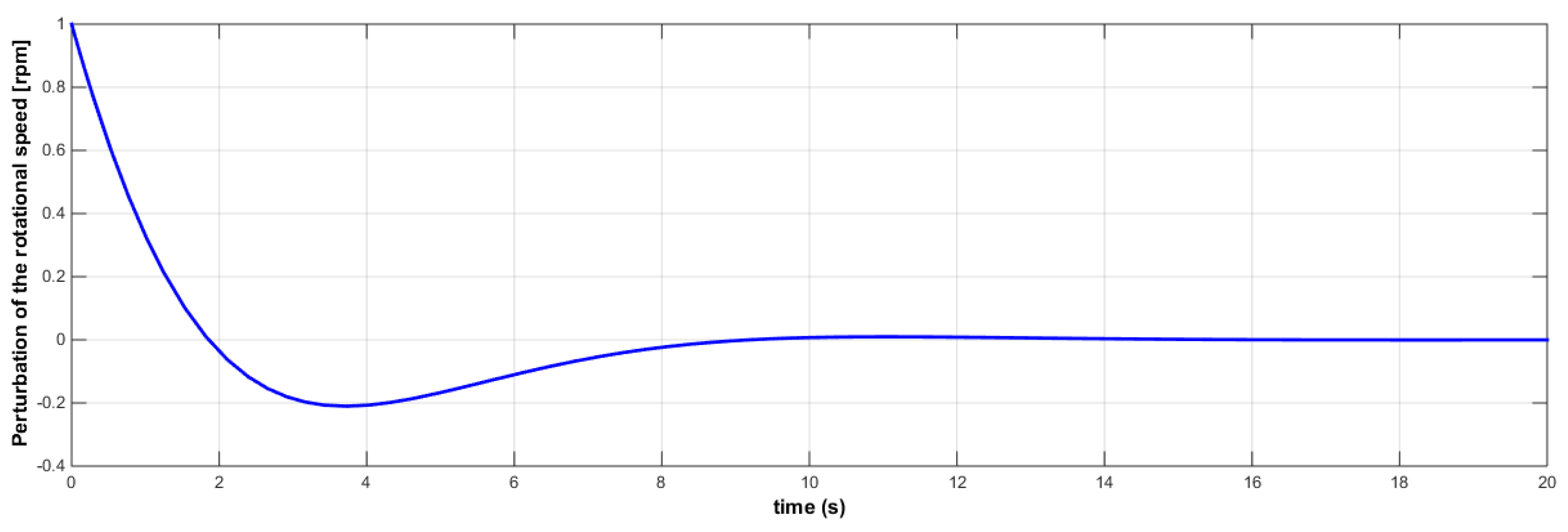
3.1.2. Low-Fidelity Model Analysis

Figure 8 shows the max $C_p$ surface plot for the NREL 5-MW reference wind turbine. The surface was obtained by simulating different rotor angular velocities and blade pitch angles in the low-fidelity aerodynamic model, for a wind velocity of 8 m/s. Through Figure 8, it is possible to see that the max $C_p$ occurs at a tip-speed ratio of 11 and a blade pitch angle of eight (deg).

The Cp-TSR-pitch surface was also analyzed for different velocities.

Table 1. Peak values of the Cp-TSR-pitch surface for different wind velocities (low-fidelity model), where the rated speed is 11.4 (m/s).

Wind Velocity (m/s)	${\mathit{C}}_{{\mathit{p}}_{\mathit{max}}}$	TSR	Blade Pitch (deg)	ω (rpm)	K (N m/(rad/s)${}^{\mathbf{2}}$)
3	0.55048	8.7965	−2.5	4	1.54 × 10${}^6$
4	0.5515	9.0713	−2.5	5.5	1.41 × 10${}^6$
5	0.55095	9.2363	−2.5	7	1.34 × 10${}^6$
6	0.55055	9.3462	−2.5	8.5	1.29 × 10${}^6$
7	0.55145	8.9535	−2.5	9.5	1.47 × 10${}^6$
8	0.5515	9.0713	−2.5	11	1.41 × 10${}^6$
9	0.55126	9.163	−2.5	12.5	1.37 × 10${}^6$
10	0.5513	8.9064	−2.5	13.5	1.49 × 10${}^6$
11	0.55153	8.9964	−2.5	15	1.45 × 10${}^6$
12	0.5515	9.0713	−2.5	16.5	1.41 × 10${}^6$

summarizes the result.

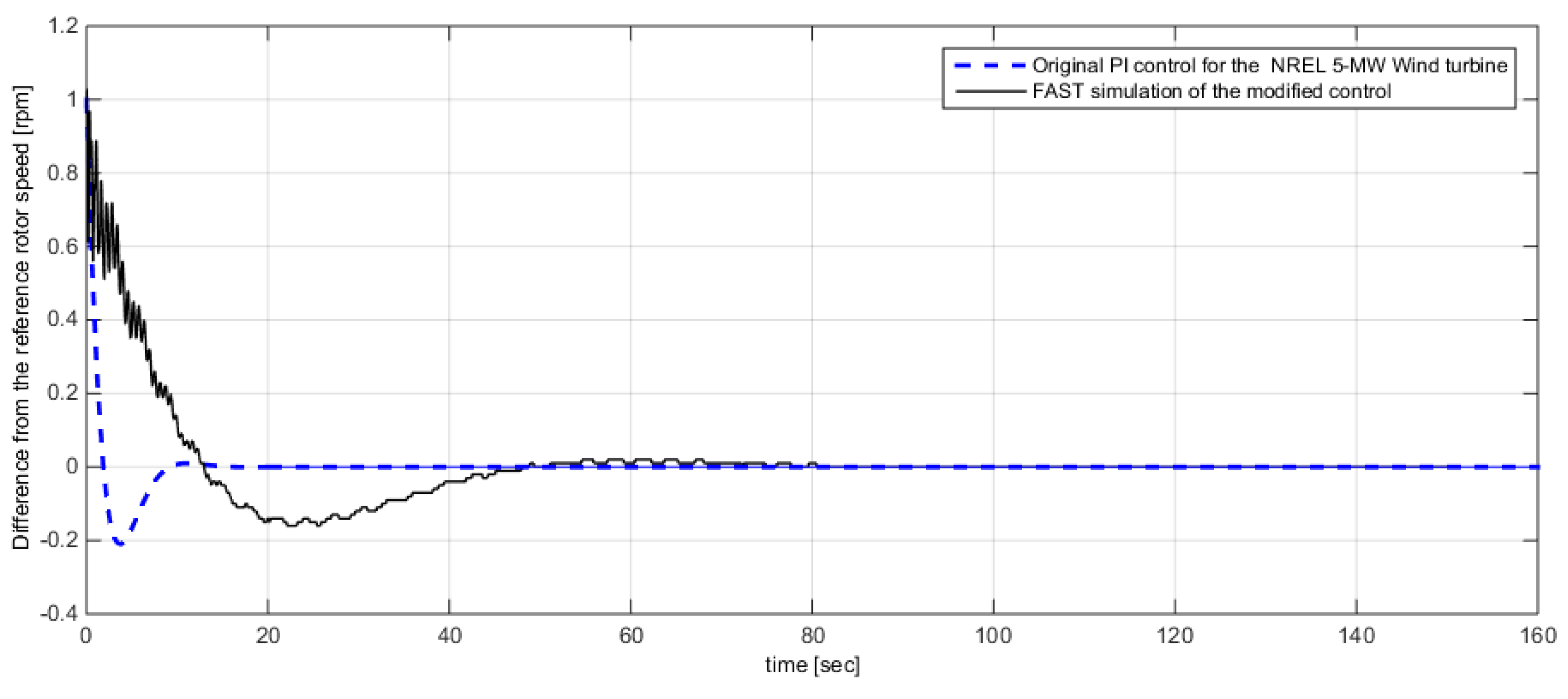
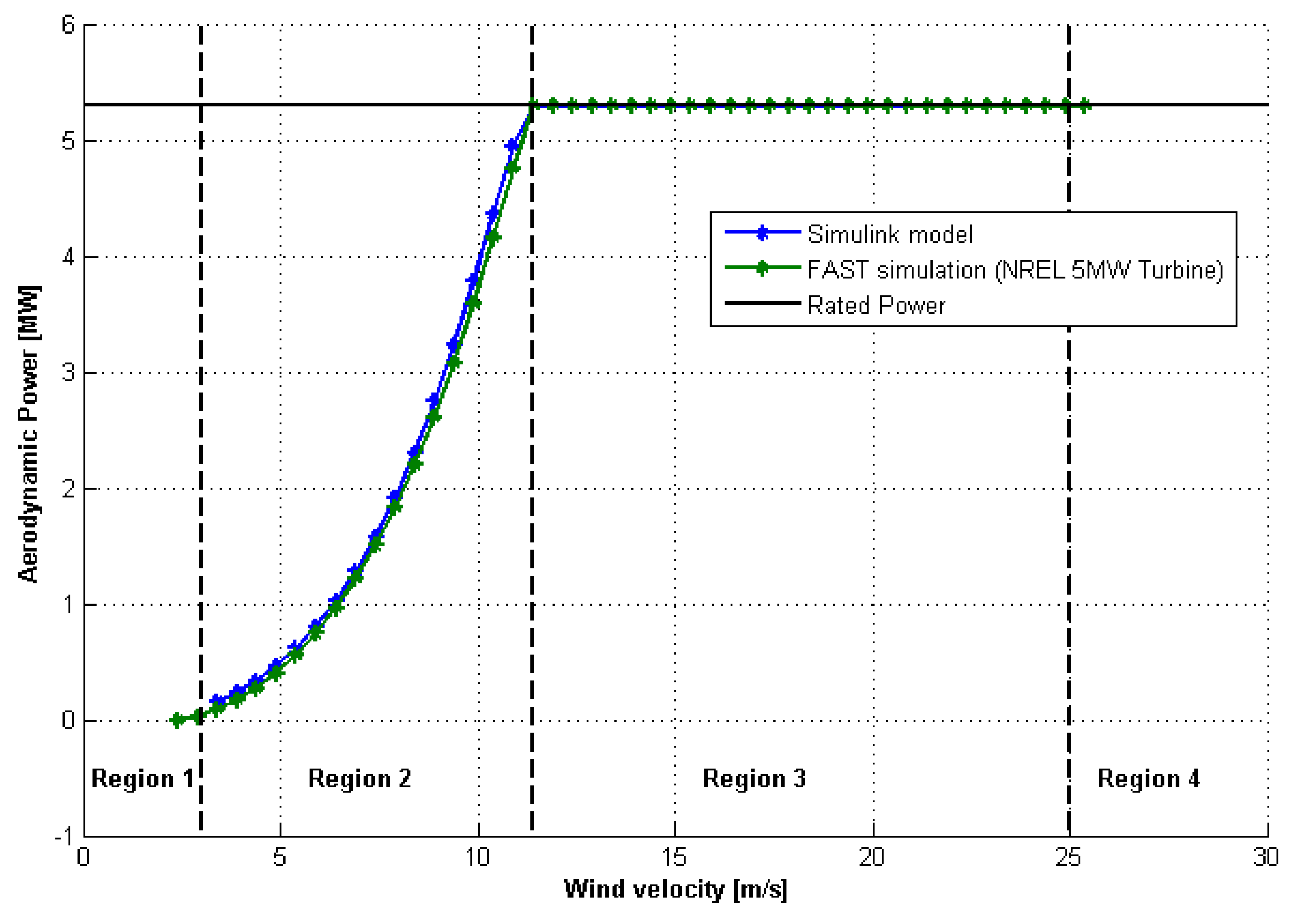
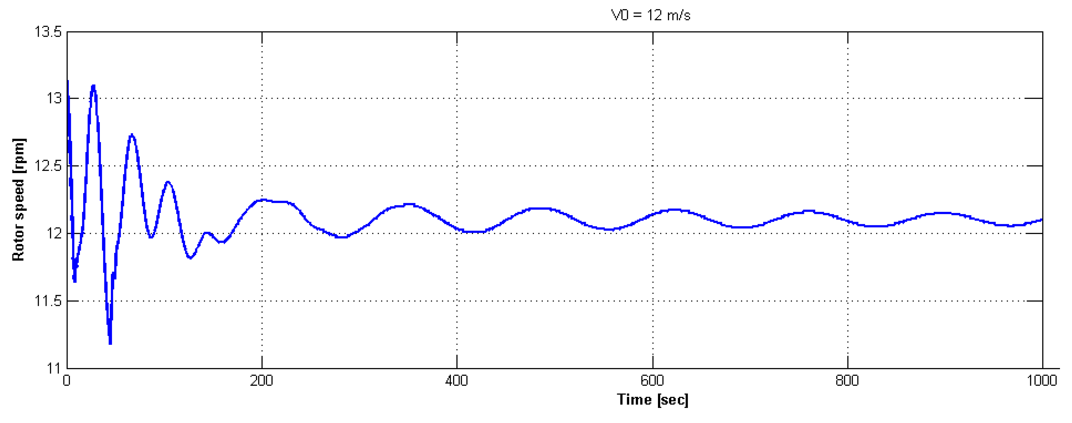
3.1.3. FAST Analysis

For obtaining the Cp-TSR-pitch surface from FAST, a different procedure was required. First, a generator torque PI controller was implemented in a closed loop with the FAST Simulink block. This controller converged the rotor angular velocity for a specified value, with the blade pitch angle held constant during the simulation. In other words, the power coefficient was calculated from a statistical inference of its settled time domain sign, for a specified rotor angular speed and blade pitch angle. Figure 9 shows the Simulink schematics.

Due to its heavy computational requirements, this analysis was made for a reduced number of points. However, we can see in Figure 10 that the peak of the surface can be identified around a pitch angle of zero degrees and a tip speed ratio of 7.5, where in the figure warm (more red) colours represent higher $C_p$ value while cold (more blue) colours represent a relatively low value.

By performing the analysis with a higher resolution around the peak of the curve, the final value for the $C_{p_{max}}$ was found. Figure 11 shows the result, where again warmer red colours represent higher $C_p$ value, while cold blue colours represent lower value of $C_p$.

Table 2. Peak values of the Cp-TSR-pitch surface for different models.

Model	${\mathit{C}}_{{\mathit{p}}_{\mathit{max}}}$	TSR	Blade Pitch	ω	K
			(deg)	(rpm)	(N m/(rad/s)${}^2$)
FAST	0.48698	7.422	−0.25	9	2.2746 × 10${}^6$
Low-fidelity model	0.5515	9.0713	−2.5	11	1.41 × 10${}^6$

compares the FAST model to the low-fidelity analysis. From the analysis of the table, we can identify the difference between the peak for the two models. This difference comes from the simplifications of the low-fidelity model, proving the importance of using FAST. However, when comparing the two models in Figure 12, we can notice that the difference is more expressive on the left side of the peak found with FAST, therefore out of the operation range of the turbine. In other words, the low-fidelity model is still a good representation of the system, but should be always compared to higher fidelity models in order to identify boundaries. In addition, the analysis performed for Figure 12 was performed for different angular velocities.

In addition, the Cp-TSR-pitch surface was performed for different wind velocities.

Table 3. Peak values of the Cp-TSR-pitch surface for different wind velocities (obtained from FAST).

Wind Velocity	${\mathit{C}}_{{\mathit{p}}_{\mathit{max}}}$	TSR	Blade Pitch	ω	K
(m/s)			(deg)	(rpm)	(N m/(rad/s)${}^2$)
4	0.4879	7.4220	−0.25	4.50	2.279 × 10${}^6$
6	0.4878	7.4220	−0.25	6.75	2.278 × 10${}^6$
8	0.4870	7.4220	−0.25	9.00	2.275 × 10${}^6$
10	0.4852	7.5869	−0.25	11.50	2.122 × 10${}^6$
12	0.4806	7.2846	−0.25	13.25	2.374 × 10${}^6$

shows the result.

3.2. High Bandwidth Blade-Pitch Control for the Onshore NREL 5-MW Wind Turbine

In [19], a Proportional-Integral (PI) controller for Region 3 was designed for the reference turbine (onshore layout) aiming for the response characteristic given by ${\omega }_n$ = 0.6 and damping ratio ζ = 0.6 to 0.7. The model is based on Equation (18) with linearized torques. Furthermore, the sensitivity of the aerodynamic power to pitch was extracted from a simplified simulation of FAST. By simulating the equations of motion in MATLAB (ode45), the behavior of the system for the wind speed of 11.4 m/s was found. The response is shown in Figure 13.

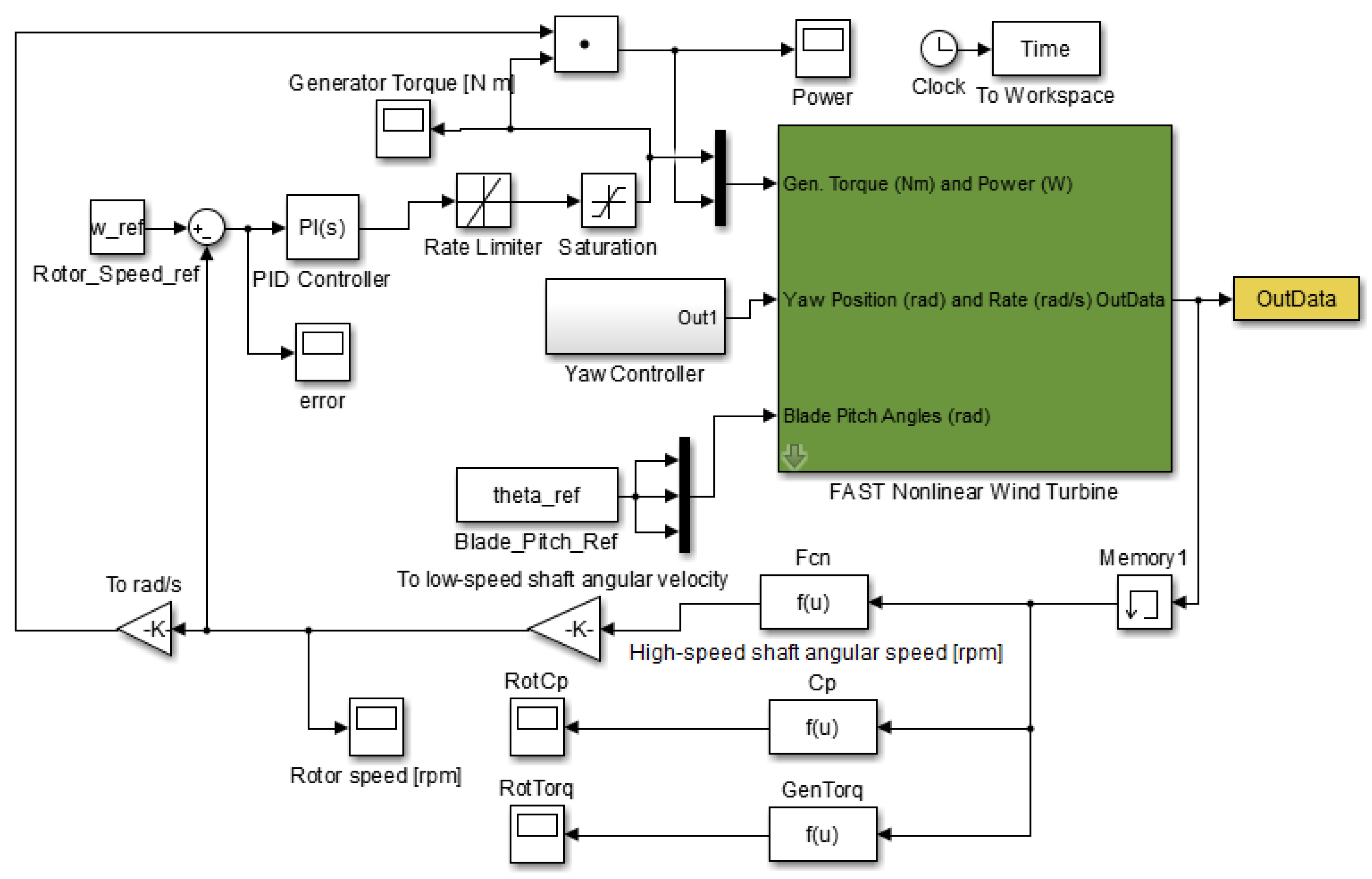
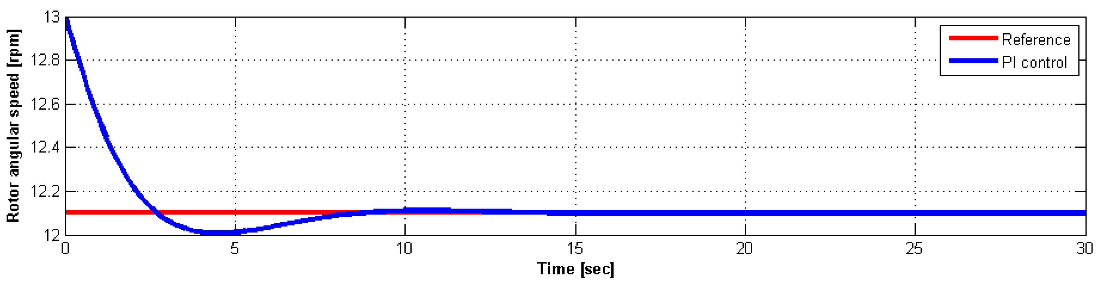
3.3. Simulink Tuned PI Blade-Pitch Control for the Onshore NREL 5-MW Wind Turbine

As stated in Ozdemir (2013) [1], a typical Region 3 controller is given by:

$$T_{gen}={\overline{T}}_{gen}$$

(26)

$${\theta }_i=\overline{\theta }+Control({\overline{\omega }}_r-{\omega }_r)$$

(27)

This approach was implemented in Simulink (as provided in Figure 14), using the dynamic of the NREL 5-MW wind turbine, the aerodynamic loads code (as an s-function block) and a tuned PI controller. The obtained results are shown in Figure 15.

3.4. Low Bandwidth Blade-Pitch Control for the Offshore NREL 5-MW Wind Turbine

The NREL 5-MW wind turbine uses a conventional variable-speed, variable blade-pitch-to-feather control system. A consequence of conventional pitch-to-feather control of wind turbines is that steady-state rotor thrust is reduced with increasing wind speed above the rated. As is well known from the literature, this effect can introduce negative damping in the system, which may lead to large resonant motions of a floating wind turbine. Analysis in the literature has demonstrated that it is important that the damping of the platform-pitch mode be positive and kept as large as possible. Hansen (2008) [18] has presented modifications to conventional wind turbine control systems that aim to eliminate the potential for negative damping of the platform-pitch mode and to improve a floating turbine system’s response. Two of these modifications were applied to the original control system for the NREL 5-MW turbine to arrive at a control system that is suitable for when the turbine is installed on the OC3-Hywind spar-buoy.

The first modification consists of a reduction of gains in the blade-pitch-to-feather control system. In an idealized PI-based blade-pitch controller, the rotor azimuth responds as a second-order system with a natural frequency and damping ratio. To maintain a reasonable relationship between the proportional and integral gains in this control system, the gains were reduced by choosing a smaller controller-response natural frequency while preserving the recommended controller damping ratio. The value selected for the baseline control system, of 0.6 rad/s, is above the platform-pitch natural frequency of about 0.21 rad/s. This relationship between frequencies has the potential to introduce negative damping of the platform-pitch mode. Larsen and Hanson (2007) [24] show that the smallest controller-response natural frequency must be lower than the smallest critical support-structure natural frequency to ensure that the support-structure motions of an offshore floating wind turbine with active pitch-to-feather control remain positively damped. Reducing the controller-response natural frequency to 0.2 rad/s will ensure that it is lower than the platform-pitch natural frequency and also lower than wave-excitation frequency of most sea states. Using the properties for the NREL 5-MW wind turbine, this frequency and the damping ratio used prior were used to derive the reduced proportional gain at minimum blade-pitch setting of 0.006275604 s and the reduced integral gain at minimum blade-pitch setting of 0.0008965149. The gain-correction factor in the gain-scheduling law of the blade-pitch controller is unaffected by this change.

The second modification applied a change to the generator-torque control strategy when operating at rated power (i.e., control Region 3). The control law in Region 3 was changed from a constant generator power to a constant generator-torque control region. The constant generator torque is set to the rated torque of 43,093.55 N/m. With this change, the generator-torque controller does not introduce negative damping in the rotor-speed response (which must be compensated by the blade-pitch controller) thus reducing the rotor-speed excursions that are exaggerated by the reduction in gains in the blade-pitch controller. This improvement however, comes at the expense of overloading of the generator, as power increases with rotor-speed excursions above the rated. Larsen and Hanson (2007) [24] have demonstrated the effectiveness of this modification. These modifications were incorporated into an updated version of the baseline control system dynamic link library (DLL) suitable for use with the floating system discussed in this report.

As we move to the offshore scenario, the previous controllers become ineffective. Therefore, [25] presents modifications on the PI control of [19], for the NREL 5-MW wind turbine mounted in an OC3-Hywind spar-buoy platform. For comparative purposes, this new approach was implemented in FAST using the onshore turbine configuration. The result is shown in Figure 16. For the same wind velocity the modified control presented ${\omega }_n=0.1095$ rad/s and $\zeta =0.6054$.

Figure 17 shows the rotational speed of the rotor of the NREL 5-MW wind turbine, mounted in an OC3-Hywind spar-buoy platform and simulated using FAST. As we can see, despite avoiding a negative damping, the low-bandwidth blade-pitch control still does not provide a competitive quality of power generation. The steady-state behavior is oscillatory, even for still water. With the presence of wind turbulence, gusts and waves, this behavior would be even worse.

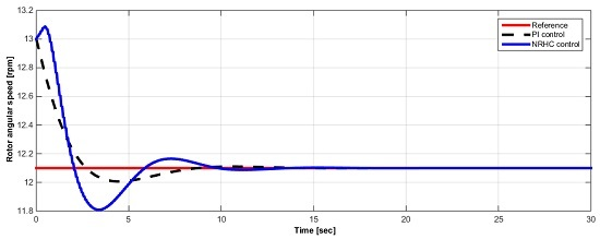
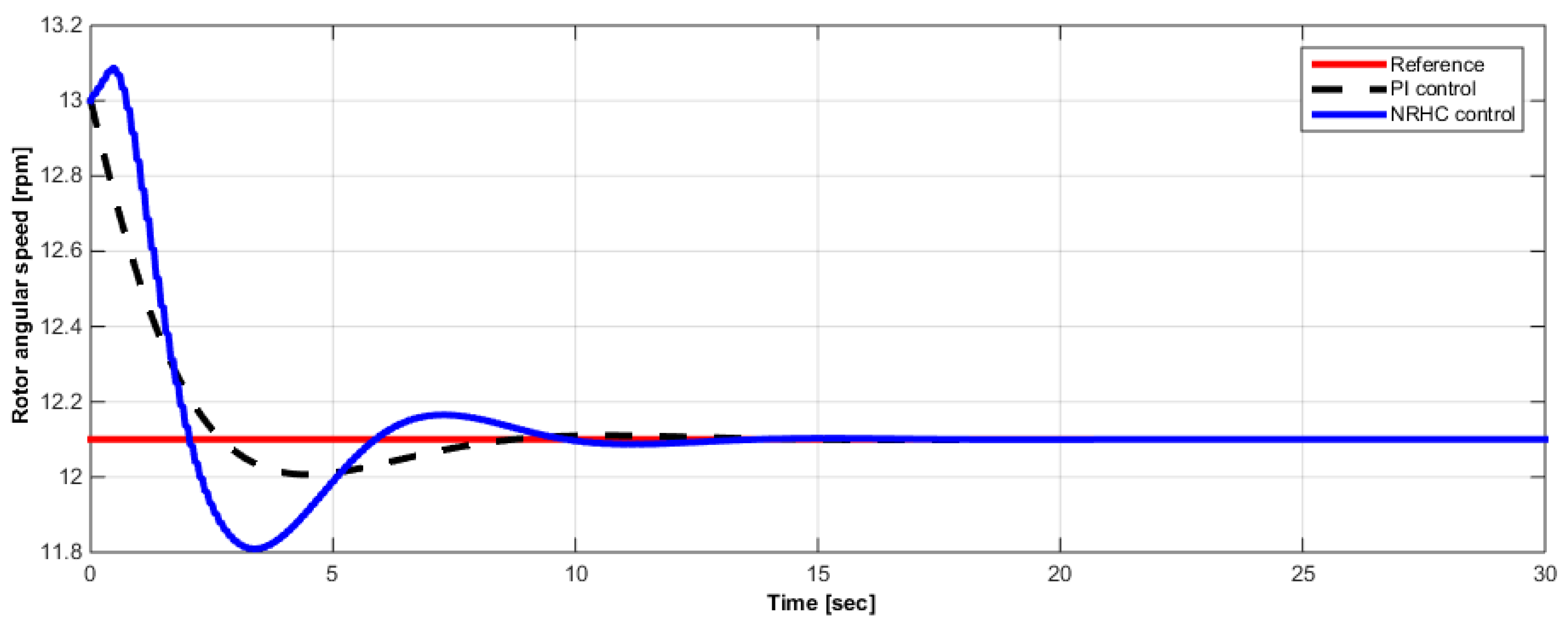
4. Real-Time NRHC Control

Different from the classical PI control methodologies, in this section, a high bandwidth blade-pitch controller for the onshore NREL 5-MW wind turbine is designed based on the real-time nonlinear receding horizon control methodology. The procedure is reduced to a family of finite horizon optimization control problems. To avoid high computational complexity, a stabilized continuation method [12,26] is employed, which is a non-iterative optimization procedure with moderate data storage capacity. Based on this method, the Nonlinear Receding Horizon Control (NRHC) problem is then solved by the backward sweep algorithm [10], in real time. The algorithm itself is executable regardless of the controllability or stabilizability of the system, which is one of the powerful aspects of the approach.

We first rewrite Equation (18) as:

$$\dot{\omega }=f(\omega (t),u(t)),$$

(28)

where $u(t)$ is the control vector that will be computed through the NRHC algorithm.

In order to utilize the real-time nonlinear receding horizon control method, the following finite horizon cost function (performance index) is proposed as follows:

$$\begin{array}{cc}\hfill J& ={\int }_t^{t+T}L[\omega (t^{\prime }),u(t^{\prime })]\mathrm{d}{t}^{\prime },\hfill \\ & ={\int }_t^{t+T}\frac{1}{2}({(\omega -{\omega }_r)}^{T}Q(\omega -{\omega }_r)+u^{T}Ru)\mathrm{d}{t}^{\prime }.\hfill \end{array}$$

(29)

Here, $Q>0$ and $R>0$ are weighting matrices, which are positive definite, and ${\omega }_r(t)$ denotes the reference trajectory of $\omega (t)$. In this specific set-up, the performance index evaluates the performance from the present time (t) to the finite future ($t+T$), where T is the horizon. The performance index is minimized for each time t starting from $\omega (t)$. Thus, the present receding horizon control problem can be converted to a family of finite horizon optimal control problems on the τ axis that is parametrized by time t. The trajectory $\omega (t+\tau )$ starting from $\omega (t)$ is denoted as $\omega (\tau ,t)$. Since the performance index of the receding horizon control is evaluated over a finite horizon, the value of the performance index is finite even if the system is not stabilizable.

Define the Hamiltonian H as follows:

$$H=L+{\Lambda }^{*T}f,$$

(30)

where Λ denotes the costate.

According to the first-order necessary conditions for $\delta J=0$, we have a two-point boundary-value problem (TPBVP) as follows:

$$\begin{array}{c}{\Lambda }_{\tau }^{*}(\tau ,t)=-H_{\omega }^T,{\Lambda }^{*}(T,t)=0,\hfill \end{array}$$

(31)

$$\begin{array}{c}{H}_u=0,\hfill \end{array}$$

(32)

where ${()}^{*}$ denotes a variable in the optimal control problem, so as to distinguish it from its correspondence in the original problem. In this notation, $H_{\omega }$ denotes the partial derivative of H with respect to ω, and so on.

In this methodology, since the state and costate at $\tau =T$ are determined by the TPBVP in Equation (31) from the state and costate at $\tau =0$, the TPBVP can be regarded as a nonlinear algebraic equation with respect to the costate at $\tau =0$ as:

$$FP(\Lambda (t),\omega (t),T,t)={\Lambda }^{*}(T,t)=0,$$

(33)

where $\Lambda (t)$ denotes the costate at $\tau =0$. The actual control input is then given by:

$$u(t)=\text{arg}\{H_u[\omega (t),\Lambda (t),u(t)]=0\}.$$

(34)

In this formulation, the optimal control $u(t)$ can be calculated from Equation (34) based on $\omega (t)$ and $\Lambda (t)$ where the ordinary differential equation of $\Lambda (t)$ can be solved numerically from Equation (33), in real time, without any need for an iterative optimization routine. Since the nonlinear equation $FP(\Lambda (t),\omega (t),T,t)$ has to be satisfied at any time t, $\frac{\mathrm{d}FP}{\mathrm{d}t}=0$ holds along the trajectory of the closed-loop system of the receding horizon control. If T is a smooth function of time t, the solution of $FP(\Lambda (t),\omega (t),T,t)$ can be tracked with respect to time. However, numerical errors associated with the solution may accumulate as the integration proceeds in practice.To resolve this issue some correction techniques are required to correct such errors in the solution. To address this problem, a stabilized continuation method [12,26,27,28] is used. According to this method, it is possible to rewrite the statement as:

$$\frac{\mathrm{d}FP}{\mathrm{d}t}=A_{s}FP,$$

(35)

where $A_s$ denotes a stable matrix to make the solution converge to zero exponentially.

In order to compute the differential equation of $\Lambda (t)$ integrated in real time, the partial differentiation of Equation (31) (with respect to time t and τ) converts the problem in hand into the following linear differential equation:

$$\frac{\partial }{\partial \tau }\left[\begin{array}{c}{\omega }_t-{\omega }_{\tau }\\ {\Lambda }_t-{\Lambda }_{\tau }\end{array}\right]=\left[\begin{array}{cc}G& -L\\ -K& -G^T\end{array}\right]\left[\begin{array}{c}{\omega }_t-{\omega }_{\tau }\\ {\Lambda }_t-{\Lambda }_{\tau }\end{array}\right]$$

(36)

where $G=f_{\omega }-f_u{H}_{uu}^{-1}{H}_{u\omega }$, $L=f_u{H}_{uu}^{-1}{f}_u^T$, $K=H_{\omega \omega }-H_{\omega u}{H}_{uu}^{-1}{H}_{u\omega }$. Since the reference trajectory ${\omega }_t(t+\tau )={\omega }_{\tau }(t+\tau )$, they are canceled in Equation (36), and the data storage is reduced.

The derivative of the nonlinear function $FP$ with respect to time is rewritten by:

$$\frac{\mathrm{d}FP}{\mathrm{d}t}={\Lambda }_t(T,t)+{\Lambda }_{\tau }(T,t)\frac{\mathrm{d}T}{\mathrm{d}t}.$$

(37)

To reduce the computational cost, the backward-sweep algorithm is employed at this point, and the relationship between the costate and other variables is expressed as:

$${\Lambda }_t-{\Lambda }_{\tau }=S(\tau ,t)({\omega }_t-{\omega }_{\tau })+c(\tau ,t),$$

(38)

where:

$$\begin{array}{cc}\hfill S_{\tau }& =-G^{T}S-SG+SLS-K,\hfill \\ \hfill c_{\tau }& =-(G^T-SL)c,\hfill \end{array}$$

(39)

In Equation (39), due to the terminal constraint on τ-axis, the following conditions hold:

$$\begin{array}{cc}\hfill S(T,t)& =0,\hfill \\ \hfill c(T,t)& =H_{\omega }^T{\mid }_{\tau =T}(1+\frac{\mathrm{d}T}{\mathrm{d}t})-A_{s}FP.\hfill \end{array}$$

(40)

Thus, the differential equation of $\Lambda (t)$ is obtained in real time as follows:

$$\begin{array}{c}\hfill \frac{\mathrm{d}\Lambda (t)}{\mathrm{d}t}=-H_{\omega }^T+c(0,t).\end{array}$$

(41)

At each time t, the Euler–Lagrange equations in Equation (31) are integrated forward along the τ axis. Equation (39) is integrated backward with terminal conditions expressed in Equation (40). Then, the differential equation of $\Lambda (t)$ is integrated for one step along the t axis so as to update the local optimal controller by Equation (34). The estimated parameters are derived from the difference between the true values and the estimation errors. If the matrix $H_{uu}$ is nonsingular, the algorithm is executable regardless of the controllability or stabilizability or the system.

In the simulation, we consider the same set-up and parameters in Section 3.2. The weighting matrices in the cost function are designed as $Q=1,R=10$. The stable matrix is designed as $A_s=-150I$.

The horizon T in the performance index is given by:

$$T(t)=T_f(1-e^{-\alpha t}),$$

(42)

where $T_f=1$ and $\alpha =0.5$.

The simulation is implemented in MATLAB, where the time step on the t axis is $0.1$ s and the time step on the artificial τ axis is $0.05$ s. The result is shown in Figure 18, where it is possible to observe that the proposed real-time nonlinear receding horizon control strategy makes the system track the reference accurately, as desired.

5. Conclusions

This work presents a detailed analysis of a simple wind turbine model, which has been validated and then used in the implementation of a nonlinear receding horizon control system. The comparison work of wind turbine dynamics is based on the model of the NREL (National Renewable Energy Laboratory) 5-MW reference wind turbine for system development, where presented results demonstrate the capability and applicability of a real-time nonlinear receding horizon control methodology on wind turbine control dynamics (in a real-time fashion). In this real-time methodology, a solution scheme of real-time nonlinear control effort is implemented, which is independent of the iterative solutions and constitutes the novelty of this work. Results provide the optimal performance of NRHC in comparison to the classical PI controller with the additional advantage of real-time tuning properties.

References

1. Ozdemir, A. Preview Control for Wind Turbines. Ph.D. Thesis, University of Minnesota, Minneapolis, MN, USA, 2013. [Google Scholar]
2. Jonkman, J.M.; Buhl, M.L., Jr. FAST User’s Guide; Technical Report No. NREL/EL-500-38230; National Renewable Energy Laboratory: Golden, CO, USA, 2005.
3. Song, Y.D.; Dhinakaran, B.; Bao, X.Y. Variable speed control of wind turbines using nonlinear and adaptive algorithms. J. Wind Eng. Ind. Aerodyn. 2000, 85, 293–308. [Google Scholar] [CrossRef]
4. Boukhezzar, B.; Houria, S. Nonlinear control with wind estimation of a DFIG variable speed wind turbine for power capture optimization. Energy Convers. Manag. 2009, 50, 885–892. [Google Scholar] [CrossRef]
5. Boukhezzar, B.; Houria, S. Nonlinear control of a variable-speed wind turbine using a two-mass model. IEEE Trans. Energy Convers. 2011, 26, 149–162. [Google Scholar] [CrossRef]
6. Beltran, B.; Tarek, A.; Mohamed, E.H.B. Sliding mode power control of variable-speed wind energy conversion systems. IEEE Trans. Energy Convers. 2008, 23, 551–558. [Google Scholar] [CrossRef] [Green Version]
7. Wu, F.; Zhang, X.P.; Ju, P.; Sterling, M. Decentralized nonlinear control of wind turbine with doubly fed induction generator. IEEE Trans. Power Syst. 2008, 23, 613–621. [Google Scholar]
8. Schlipf, D.; Schlipf, D.J.; Kühn, M. Nonlinear model predictive control of wind turbines using LIDAR. Wind Energy 2013, 16, 1107–1129. [Google Scholar] [CrossRef]
9. Galvani, P.A.; Sun, F.; Turkoglu, K. Aerodynamic Modelling of the 5-MW Wind Turbine for Development and Application of Real-Time Nonlinear Receding Horizon Control. In Proceedings of the AIAA Modeling and Simulation Technologies Conference, San Diego, CA, USA, 4–8 January 2016; p. 173.
10. Bryson, A.; Ho, Y. Applied Optimal Control; Hemisphere: New York, NY, USA, 1975. [Google Scholar]
11. Chen, C.; Shaw, L. On receding horizon feedback control. Automatica 1982, 18, 349–352. [Google Scholar] [CrossRef]
12. Ohtsuka, T.; Fujii, H. Real-Time Optimization Algorithm for Nonlinear Receding-Horizon Control. Automatica 1999, 33, 1147–1154. [Google Scholar] [CrossRef]
13. Thomas, Y. Linear quadratic optimal estimation and control with receding horizon. Electron. Lett. 1975, 11, 19–21. [Google Scholar] [CrossRef]
14. Kwon, W.; Bruckstein, A.; Kailath, T. Stabilizing state-feedback design via the moving horizon method. Int. J. Control 1983, 37, 631–643. [Google Scholar] [CrossRef]
15. Mayne, D.; Michalska, H. Receding horizon control of nonlinear systems. IEEE Trans. Autom. Control 1990, 35, 814–824. [Google Scholar] [CrossRef]
16. Mayne, D.; Michalska, H. An implementable receding horizon controller for stabilization of nonlinear systems. In Proceedings of the 29th IEEE Conference Decision and Control, Honolulu, HI, USA, 5–7 December 1990; pp. 3396–3397.
17. Moriarty, P.J.; Hansen, A.C. AeroDyn Theory Manual; National Renewable Energy Laboratory: Golden, CO, USA, 2005.
18. Hansen, M.O. Aerodynamics of Wind Turbines; Routledge: London, UK, 2008. [Google Scholar]
19. Butterfield, S.; Musial, W.; Scott, G. Definition of a 5-MW Reference Wind Turbine for Offshore System Development; National Renewable Energy Laboratory: Golden, CO, USA, 2009.
20. Fischer, B. Reducing rotor speed variations of floating wind turbines by compensation of non-minimum phase zeros. IET Renew. Power Gener. 2013, 7, 413–419. [Google Scholar] [CrossRef]
21. Jonkman, J.M. Dynamics Modeling and Loads Analysis of an Offshore Floating Wind Turbine. Ph.D. Thesis, University of Colorado, Boulder, CO, USA, 2007. [Google Scholar]
22. Miller, N.W.; Price, W.W.; Sanchez-Gasca, J.J. Dynamic Modeling of GE 1.5 and 3.6 Wind Turbine-Generators. In GE-Power Systems Energy Consulting; General Electric Company: Schenectady, NY, USA, 2003. [Google Scholar]
23. Johnson, K.E. Adaptive Torque Control of Variable Speed Wind Turbines; National Renewable Energy Laboratory: Golden, CO, USA, 2004; pp. 54–57.
24. Larsen, T.J.; Hanson, T.D. A method to avoid negative damped low frequent tower vibrations for a floating, pitch controlled wind turbine. J. Phys. Conf. Ser. 2007, 75, 12073. [Google Scholar] [CrossRef]
25. Jonkman, J.M. Definition of the Floating System for Phase IV of OC3; National Renewable Energy Laboratory: Golden, CO, USA, 2010.
26. Ohtsuka, T. Time-variant receding-horizon control of nonlinear systems. J. Guid. Control Dyn. 1998, 21, 174–176. [Google Scholar] [CrossRef]
27. Kabamba, P.; Longman, R.; Sun, J.-G. A homotopy approach to the feedback stablilization of linear systems. J. Guid. Control Dyn. 1987, 10, 422–432. [Google Scholar] [CrossRef]
28. Ohtsuka, T.; Fujii, H. Stabilized continuation method for solving optimal control problems. J. Guid. Control Dyn. 1994, 17, 950–957. [Google Scholar] [CrossRef]
Figure 1. Systematic procedure flowchart that is implemented in determining the behavior of the turbine.
Aerospace 03 00027 g001
Figure 2. NREL (National Renewable Energy Laboratory) 5-MW wind turbine mounted on the OC3-Hywind spar buoy platform.
Aerospace 03 00027 g002
Figure 3. Aerodynamic power curve of the rotor of the NREL 5-MW wind turbine.
Aerospace 03 00027 g003
Figure 4. Aerodynamic power curve of the rotor of the NREL 5-MW wind turbine, based on controlled operation points.
Aerospace 03 00027 g004
Figure 5. Controlled power curve of the NREL 5-MW wind turbine.
Aerospace 03 00027 g005
Figure 6. Actuator dynamics.
Aerospace 03 00027 g006
Figure 7. Response of the generator-torque control.
Aerospace 03 00027 g007
Figure 8. Cp-TSR-pitch surface for the NREL 5-MW reference wind turbine for a wind velocity of 8 m/s.
Aerospace 03 00027 g008
Figure 9. Generator torque control developed to obtain the Cp-TSR-pitch surface from FAST.
Aerospace 03 00027 g009
Figure 10. Cp-TSR-pitch surface for the NREL 5-MW reference wind turbine for a wind velocity of 8 m/s, obtained from FAST.
Aerospace 03 00027 g010
Figure 11. Cp-TSR-pitch surface for the NREL 5-MW reference wind turbine for a wind velocity of 8 m/s, obtained from FAST.
Aerospace 03 00027 g011
Figure 12. Comparison between the low-fidelity model and FAST.
Aerospace 03 00027 g012
Figure 13. Dynamic behavior of NREL 5-MW under small perturbation of the low-speed shaft rotational speed about the rated speed of 12.1 rpm.
Aerospace 03 00027 g013
Figure 14. Simulink implementation.
Aerospace 03 00027 g014
Figure 15. Dynamic behavior of the NREL 5-MW under small perturbation of the low-speed shaft rotational speed based on the PI control methodology.
Aerospace 03 00027 g015
Figure 16. Original PI control for the NREL 5-MW wind turbine versus modified PI control. Wind velocity of 11.4 m/s.
Aerospace 03 00027 g016
Figure 17. NREL 5-MW wind turbine mounted in an OC3-Hywind spar-buoy platform. Wind velocity of 12 m/s. Still water.
Aerospace 03 00027 g017
Figure 18. Dynamic behavior of the NREL 5-MW under small perturbation of the low-speed shaft rotational speed by the real-time nonlinear receding horizon control methodology, in comparison to PI control.
Aerospace 03 00027 g018