Optimization of a Human-Powered Aircraft Using Fluid–Structure Interaction Simulations

Abstract

The special type of aircrafts in which the human power of the pilot is sufficient to take off and sustain flight are known as Human-Powered Aircrafts (HPAs). To explore the peculiarities of these aircrafts, the aerodynamic performance of an existing design is evaluated first, using both the vortex lattice method and computational fluid dynamics. In a second step, it is attempted to design and optimize a new HPA capable of winning the Kremer International Marathon Competition. The design will be special in that it allows one to include a second pilot on board the aircraft. As the structural deflection of the wing is found to be a key aspect during design, fluid–structure interaction simulations are performed and included in the optimization procedure. To assess the feasibility of winning the competition, the physical performance of candidate pilots is measured and compared with the predicted required power.

1. Introduction

By careful design, human power is found sufficient to propel an aircraft. These special aircrafts, known as Human-Powered Aircrafts (HPAs), are extremely light, fly at very low speeds and are usually constructed for a single pilot.

One of the most sophisticated HPAs is the Daedalus from the Massachusetts Institute of Technology (MIT). It was built in an attempt to recreate the mythical escape of its namesake, said to have built himself wings of feathers and wax. After years of intensive design and testing with a prototype aircraft, the Daedalus was finally ready in 1988 for a legendary flight across the Aegean Sea from Crete to Santorini. The flight covered a distance of 74 miles (119 km), completed in three hours 54 minutes, the longest time and distance flown under human power up to date [1]. The Daedalus can be seen in Figure 1.

Given its outstanding performance, the first part of this work is devoted to analyzing this HPA. More specifically, the Daedalus will be simulated in two different software. The first software is AVL [2], which performs aerodynamic analyses based on the Vortex Lattice Method (VLM). This software is developed by MIT and is publicly available. For the second simulation, the Computational Fluid Dynamics (CFD) software STAR-CCM+ is used, which will solve the Reynolds-averaged Navier–Stokes equations. The main purpose of this first part is to have an idea of the capabilities of both software and to verify their accuracy by comparing the results with other data.

In the second part, it is attempted to design and optimize an HPA ourselves using AVL and MATLAB. The design will be special in that the HPA should be capable of winning the Kremer International Marathon Competition. This is a prestigious challenge set out by Henry Kremer in which a specific course is to be flown in less than one hour. The course is illustrated in Figure 2 and consists of two laps of the outer circuit, followed by a figure-eight and two more outer circuits. As such, the total distance is approximately the distance of a marathon. More details can be found in [3].

As can be seen in Figure 1, the wing experiences a large deformation during flight. This deformation is actually desired for stability reasons and should therefore be carefully designed. To take this aspect into account during the optimization of our own HPA, Fluid–Structure Interaction (FSI) simulations of the wing will be performed coupling AVL and MATLAB. Simulations [4,5] and experiments [6] of FSI are currently also used to optimize commercial aircrafts. Furthermore, the deflection of a wing can be used to reduce its sensitivity to wind gusts [7].

Another special feature of our design is the possibility of adding a second pilot on board the aircraft. As such, it will be investigated if powering an HPA by two pilots offers some advantages compared to a single pilot.

In the final part, a CFD simulation of the optimized design is performed in STAR-CCM+. Additionally, the physical performance of our candidate pilots is measured. Using these data, it will be verified if sufficient human power can be generated in order to complete the Kremer International Marathon Course within time.

2. The Daedalus Models

As a first step, a 3D CAD model of the Daedalus is constructed, which will give a clear overview of its geometry. This CAD model is further used for the CFD simulation in STAR-CCM+. To perform the simulation in AVL, a second and simplified model will have to be constructed, as further explained.

2.1. CAD Model

Most of the geometrical and structural data concerning the Daedalus are made publicly available by MIT [8]. Based on these data, a precise replicate was constructed, which can be seen in Figure 3. The Daedalus has a wingspan of 112 ft (34 m), being as large as the wingspan of a Boeing 737-800. The corresponding wing area is 332 ft${}^2$ (31 m${}^2$), resulting in a mean chord length of 2.96 ft (0.90 m). For increased aerodynamic performance, the wing is highly tapered, the ratio of the chord length at the tip to root $(c_{\mathrm{tip}}/c_{\mathrm{root}})$ being equal to 1/3. Due to the tapering, there is a large variation in the chord Reynolds number $R{e}_c$, such that the wing is made up of four different airfoils (Daedalus (DAE) airfoils by Mark Drela, namely DAE11, DAE21, DAE31, DAE41), each optimized for a different Reynolds numbers [9]. During flight, the wing is designed to have a tip deflection of 2 m at a cruise speed of 6.7 m/s [10]. As only the tip deflection was specified, the deformation of the complete wing is assumed as parabolic. The fuselage is the aerodynamic structure surrounding the pilot and is located just underneath the wing. The airfoil used to construct the fuselage was not specifically given, but is assumed to be the symmetrical NACA65${}_4$-021. Since the Daedalus was designed for long, straight flights, it required no ailerons for its control; steering was accomplished by the all-moving rudder and elevator. These are respectively the vertical and horizontal surfaces of the tail and are assumed to be constructed of the symmetrical NACA0010. The final structure is the tail boom, a carbon fiber tube going from the nose of the aircraft to its tail, used to connect the different parts of the aircraft. The propeller mounted in front of the aircraft will not be simulated in this work, but will be taken into account in the form of a propulsive efficiency.

2.2. AVL Model

When the flow is considered as steady, incompressible, inviscid and irrotational, it can be described by Laplace’s equation:

$${\nabla }^2\mathsf{\Phi }=0$$

(1)

in which $\overrightarrow{v}=\nabla \mathsf{\Phi }$ and where $\overrightarrow{v}$ represents the velocity field. As the boundary condition on a wall, it holds:

$$\nabla \mathsf{\Phi }·\overrightarrow{n}=0$$

(2)

which states that the normal component of the velocity on the wall must be zero. To solve Laplace’s equation numerically, the vortex lattice method can be applied. In this method, every aerodynamic structure (wing, fuselage, rudder and elevator) should first be represented as a thin surface, located along its camber lines. In AVL, the different structures are defined by specifying a number of sections, each characterized by the type of airfoil, the chord length, the position of the leading edge and the incidence, which are then linearly interpolated. By defining the structures in this way, the camber lines are easily determined together with the thin surfaces. These thin surfaces are now further divided into smaller elements, both in the spanwise and chordwise direction. Figure 4 shows the AVL model of the Daedalus plotted on top of its CAD model. Note that as the tail boom does not consist of airfoil sections, it cannot be included in the AVL model.

The principle of the vortex lattice method is now briefly explained, and the reader is referred to [11] for more details. In every element, a horseshoe vortex is defined, which is characterized by a certain strength. The horseshoe vortices will each induce a velocity field according to the Biot–Savart law and which is proportional to their strength. The problem now consists of finding the strengths of every horseshoe vortex, such that the boundary condition in Equation (2) is fulfilled. Once the strengths are known, it is possible to calculate the lift and induced drag of every element.

In order to take the profile drag (viscous + pressure drag) into account, AVL has the option to include the drag polar of every section used in defining the geometry. To see how it is done, consider Figure 5, showing the drag polar of the airfoil DAE11, in this case for a chord Reynolds number of 500,000. This drag polar was constructed using the panel code XFOIL [12]. To define this drag polar in AVL, three specific points should be determined; negative stall, minimal drag and positive stall. These points are indicated in the figure and should be given to AVL. Based on these three points, AVL will now construct two parabolic curves, each starting in the point of minimal drag. As such, the actual drag polar is slightly approximated as shown in the figure. Note that a specific drag polar will have to be defined for every section, which will depend on its type of airfoil and its chord Reynolds number.

Finally, to determine the equilibrium position of the Daedalus at a certain flight velocity, AVL requires its mass and Center of Gravity (CG). Based on the structural data provided by MIT, the mass and CG of the different structures were determined and are summarized in

Table 1. Mass and Center of Gravity (CG) breakdown of the Daedalus.

Name	Mass (kg)	${\mathbf{x}}_{\mathit{CG}}$ (m)	${\mathbf{y}}_{\mathit{CG}}$ (m)	${\mathbf{z}}_{\mathit{CG}}$ (m)
Wing	17.10	0	0	0.94
Fuselage	1.91	0.76	0	−0.85
Elevator	0.52	5.33	0	0.31
Rudder	0.52	6.10	0	0.26
Tail boom	1.49	1.55	0	0
Propeller	1.36	−1.98	0	0
Gearbox	0.91	−0.91	0	0
Crank set	1.36	−0.91	0	−1.52
Water	5.44	−0.06	0	−1.68
Pilot	74.84	0	0	−1.22
Daedalus	105.44	0.04	0	−0.83

. Note that the empty weight of the Daedalus, so without the pilot, is equal to just 30.60 kg. This means that the pilot (74.84 kg) is almost 2.5-times heavier than the aircraft itself. In equilibrium, the total lift should equal the weight of the Daedalus, and the pitching moment around its CG should be zero. This can be accomplished by adjusting the Angle of Attack (AoA) of the aircraft and the local AoA of the elevator. These two angles will be a direct output of AVL, together with the induced and profile drag when the drag polars have been included.

2.3. Two-Dimensional Computational Fluid Dynamics (CFD) Model

As HPAs fly at very low speeds (around 6.7 m/s in the case of the Daedalus), their corresponding chord Reynolds numbers are mostly well below one million. The result is that the flow will remain laminar over a noticeable fraction of the airfoil and that the transition process from laminar to turbulent will take place in the form of a so-called laminar separation bubble. This phenomenon is illustrated in Figure 6.

To predict this phenomenon in CFD, two models will be used; the k-ω shear stress transport (SST) turbulence model and the γ-Re${}_{\theta }$ transition model. The γ-Re${}_{\theta }$ transition model is based on a correlation and will predict the onset of transition. In order to investigate the accuracy of the γ-Re${}_{\theta }$ transition model, some 2D simulations of an airfoil will be performed first and compared with experimental data from wind tunnel tests performed at UIUC (University of Illinois at Urbana-Champaign). The investigated airfoil is the FX63-137, specifically designed for low Reynolds numbers and used in some early HPA designs. For the 2D simulations, a circular fluid domain is considered, with a radius of 50 chord lengths and the airfoil located in the center. The outer boundary is cut at +45 and −45 degrees starting from the trailing-edge side, allowing one to define a velocity inlet and pressure outlet. All simulations are performed at a Reynolds number of 500,000. The fluid domain is now discretized, in which the 2D mesh is actually derived from a 3D mesh. More specifically, using the trimmed hexahedral mesher of STAR-CCM+, a 3D mesh is first constructed around a wing. This wing has a chord length of unity and is made up of the airfoil FX63-137. By now, considering a specific section of this 3D mesh, the 2D mesh is obtained. The advantage of this 2D mesh is that it will allow one to evaluate the quality of the 3D mesh. This is useful, as a trimmed hexahedral mesh will later on be constructed around the complete Daedalus. In order to explore the full capability of the γ-Re${}_{\theta }$ transition model, the trimmed hexahedral mesh was constructed with an extremely fine boundary layer mesh, shown in Figure 7.

This boundary layer mesh consists of a 30-layer, 30 mm-thick inflation layer, hyperbolically extruded. Its first cell height is 0.01 mm, assuring a y${}^{+}<1$, which is needed in order to properly resolve the boundary layer. To determine the precise location of transition, a chordwise spacing of 1 mm is applied. The complete 2D mesh consists of 93,000 cells. The flow is further modeled as incompressible, justified by the very low Mach numbers of HPAs, and additionally, the turbulent intensity is set to 0.07% together with a turbulent viscosity ratio of 10.

2.4. Three-Dimensional CFD Model

As outlined, the objective is to simulate the entire Daedalus in CFD. However, using its symmetry, half of the aircraft will be sufficient. For this simulation, the fluid domain is constructed as a half-sphere with a radius of 100 m. The outer boundary is again split into a velocity inlet and a pressure outlet. Using the trimmed hexahedral mesher, the complete fluid domain is discretized and is shown in Figure 8. The boundary layer mesh is somewhat coarser, to limit the number of cells, but still provides sufficient accuracy. It consists of a 15-layer, 20 mm-thick inflation layer, in which the maximal edge size of the elements on the geometry is 5 mm. The complete mesh consists of 52 million cells.

3. The Daedalus Results

For a clear overview, the results of the different models are discussed in separate sections. The two-dimensional CFD simulations are analyzed first and will provide additional insight when later on analyzing the three-dimensional simulations of the Daedalus in AVL and STAR-CCM+.

3.1. Results of Two-Dimensional CFD

The results of the 2D CFD simulations can be seen in Figure 9. In addition to the experimental data and CFD simulations using the γ-Re${}_{\theta }$ transition model, the results have been added of CFD simulations using the k-ω SST turbulence model without transition together with the results of the panel code XFOIL. The 2D CFD simulations were performed transiently, in which the solution was found to be steady after approximately 10 s in all of the cases considered. The time step was taken as 0.01 s. Figure 9a shows the lift coefficient $C_L$ versus the angle of attack α. The CFD simulations using the transition model are seen to agree the closest with the experimental data and show a slight overprediction for positive angles of attack. The results of CFD without transition and XFOIL are seen to respectively underestimate and overestimate the lift for all angles of attack considered. Further, in Figure 9b, the drag coefficient $C_D$ is shown as a function of the angle of attack. CFD with transition and XFOIL show a comparable accuracy for angles of attack between zero and six degrees, in which XFOIL is found to be more accurate beyond this range. Note that there is a consistent overprediction by CFD with transition and underprediction by XFOIL. Neglecting the transition phenomenon results in a heavy overprediction of the drag. For positive angles of attack, this overprediction is found to be more than 50%. It is clear that the Daedalus will have to be simulated using a transition model, in order to obtain accurate results. Using the top two figures, the drag polar can now be constructed, which is shown in Figure 9c. CFD with transition is seen to agree well with the experimental data, especially for positive angles of attack. Due to the consistent overprediction of the lift and underprediction of the drag made by XFOIL, the corresponding drag polar is seen to have the same shape as the experimental data, but is shifted upwards. For positive angles of attack, this leads to an underestimation of the drag coefficient as a function of the lift coefficient. As an example, for a lift coefficient of 1.4, the underprediction with respect to the experimental data is found to be 14%. Finally, Figure 9d shows the lift-to-drag ratio versus the angle of attack. CFD with transition is seen to agree well, but predicts a somewhat lower maximal value of $L/D$.

In Figure 10a, the pressure coefficient around the airfoil is given at zero degrees angle of attack. The pressure distributions predicted by CFD with the transition model and XFOIL clearly show the presence of a laminar separation bubble on both the suction and pressure side of the airfoil. When comparing the enclosed surfaces of the different pressure distributions, a clear difference is observed. XFOIL is seen to have the largest enclosed surface, followed by CFD with transition and CFD without transition. However, this observation is in agreement with the lift predictions at zero degrees angle of attack shown in Figure 9a. To see the key difference between the two CFD models, consider Figure 10b, showing the turbulent kinetic energy around the airfoil. In CFD without transition (upper airfoil), the production of turbulent kinetic energy is directly initiated at the leading edge of the airfoil and increases towards the trailing edge. In CFD with transition (lower airfoil), the production is only initiated after the laminar flow has locally detached (Figure 6). From the moment the detached flow becomes sufficiently turbulent, it will reattach, corresponding with a peak in turbulent kinetic energy.

3.2. Results of AVL

The results of the AVL simulation of the Daedalus are given in

Table 2. Comparison estimated performance of the Daedalus.

Property	MIT [15]	AVL Model	CFD Model
Flight Velocity (m/s)	6.7	6.7	6.7
Gliding Drag (N)	27	22.2	26.2
Induced (N)	10.5 (35%)	11.2	−
Profile (N)	12.0 (40%)	9.7	−
Parasite (N)	4.5 (15%)	1.3	2.5
Lift (N)	1034.4	1034.4	1034.8
Propulsive Efficiency	0.90	0.90	0.90
Pilot Power (W)	201	165	195
AoA Aircraft (${}^{\circ }$)	−	2.76	2.76
AoA Elevator (${}^{\circ }$)	−	−4.6	−4.6
Calculation time	−	9.94 s	1 day

. The simulation was performed at the design flight velocity of 15 mph (6.7 m/s), in which the Daedalus was found to fly at an angle of attack of 2.76 degrees in order to generate sufficient lift. Additionally, for the pitching moment to be zero, the elevator had to be trimmed to a negative angle of −4.6 degrees. At this equilibrium position, the total drag was calculated together with its components. Note that this total drag corresponds with the so-called gliding drag of the aircraft, as no propulsion is simulated in AVL.

For the different drag components listed, it is important to know that the induced drag and profile drag only refer to the wing of the Daedalus and that the parasite drag is the difference between the gliding drag and the drag of the wing. Based on the gliding drag and the propulsive efficiency, consisting of the mechanical and propeller efficiency, the corresponding pilot power is determined. This is thus the actual power that the pilot will have to deliver to keep the aircraft up in the air.

At this point, a comparison can be made with the data from MIT, which is also included in Table 2. It is important to emphasize that the data from MIT are also estimates, but nevertheless, they provide an idea of the actual drag and its components. Comparing the induced drag, AVL is found to predict a somewhat larger value (7%), but is still a reasonable prediction. However, comparing the profile and parasite drag, these are seen to be substantially underpredicted. In the case of the profile drag, the underprediction is found to be 19%. Recall that AVL determines the profile drag based on the local lift coefficients of the different sections and the corresponding drag polars generated by XFOIL. In the previous section, the drag polar of XFOIL (Figure 9c) was seen to underestimate the profile drag for the airfoil FX63-137. This underprediction is also observed in other work for different airfoils [13,14]. As such, the underprediction of the wing’s profile drag in AVL was to be expected. Before making any conclusions on the performance of AVL, let us first examine the results of the CFD simulation.

3.3. Results of Three-Dimensional CFD

The CFD simulation of the Daedalus was performed steadily in which its configuration was adjusted to be identical as in AVL. As such, the angle of attack of the aircraft and elevator was the same in both simulations. The results of the CFD simulation can be found in Table 2. The generated lift is seen to agree extremely well, such that the Daedalus is also in equilibrium in the CFD simulation. Comparing the total drag of the wing, being 23.7 N in the CFD simulation versus 22.5 N estimated by MIT, the value is seen to agree within 5%. Note that 90% of the gliding drag is due to the wing. As for the AVL simulation, the parasite drag is strongly underpredicted. However, some simplifications were made to both models of the Daedalus, resulting in a somewhat lower parasite drag. In both models, the external lift wires of the Daedalus (Figure 11) were not included, and the fuselage was made slightly more aerodynamic. In reality, the fuselage contained a ventilation opening to draw in air for the pilot and had an additional structure mounted on its nose to drive the propeller (as can be seen in Figure 1). Recall that in the AVL model, also the tail boom is left out. Comparing the pilot power, the CFD simulation is seen to agree within 3% with the value of MIT. Therefore, although there is a slight overprediction of the total drag of the wing and a noticeable underprediction of the parasite drag, the CFD simulation provides a very reasonable estimate of the pilot power.

In Figure 12, the turbulent kinetic energy is shown close to the surface of the Daedalus together with the constrained streamlines, which help in visualizing the laminar separation bubble. At the position where the streamlines seem to be halted for the first time, the flow locally detaches, and at the position of peak turbulent kinetic energy, the flow reattaches. The size of the laminar separation bubble on the wing is seen to be approximately constant along its span, except near the wingtip. Note that the pressure side of the wing is completely laminar. The flow around the rudder is clearly influenced by the wake of the wing, in which the midsection is seen to be fully turbulent, whereas the upper section is largely laminar with transition occurring near the trailing edge.

As a small conclusion, the CFD simulation in STAR-CCM+ is seen to predict the pilot power very accurately, but requires a large amount of computational power and time for a single simulation (Table 2). The contrary is observed in AVL, where the pilot power is underpredicted by about 18%, but the calculation time is in the order of seconds. Given this very short calculation time, AVL will be used for the optimization our own HPA in the following part. Only the final optimized design will be simulated in STAR-CCM+, which will give an accurate prediction of the required pilot power.

4. Optimization: Method and Cases

It was shown in Table 2 that the drag of the wing is the main contributor to the aircraft’s total drag. As such, the first step in designing our HPA for the Kremer International Marathon Competition will consist of optimizing a wing, both geometrically and structurally. Figure 13 provides an overview of how the mechanical structure of a wing is optimized for a given wing geometry. This structural optimization procedure is explained in detail in the following sections.

4.1. Wing Geometry

In the undeformed state, the outer geometry of the wing is described by its airfoil, span b, tip chord length $c_{\mathrm{tip}}$, taper ratio λ $(c_{\mathrm{tip}}/c_{\mathrm{root}})$, twist angle θ and the relative position $x/c$ of the spar’s center. These design variables are indicated on half of a wing in Figure 14. The spar is a straight thin-walled circular tube, and its relative position $x/c$ is assumed constant along the wing. Furthermore, only one type of airfoil is used for the entire wing, and the variation in chord length is linear from root to tip.

4.2. AVL

For a given wing geometry defined by the aforementioned design variables, an initial simulation is performed in AVL. In order to perform the simulation, two conditions have to be defined; the flight velocity and the desired lift. The flight velocity follows from the challenge of completing a marathon distance (42,195 m) in less than one hour. This results in a minimal flight velocity of 11.72 m/s. However, the flight velocity is safely rounded to 12 m/s. For the desired lift, it is assumed that the wing must generate just enough lift to carry the mass of the pilot(s) and the mass of the complete aircraft structure. At this moment, the mass of the aircraft is still unknown, such that the mass of the Daedalus (30.60 kg) is taken as an initial guess for an HPA for one pilot, and an additional 10 kg is added in the case of an HPA for two pilots. Once both conditions are specified, AVL will determine the required angle of attack of the wing. The results of interest are now the total drag (induced + profile drag) of the wing and the so-called strip forces, being the resultant forces acting on every spanwise strip of the wing. These are schematically illustrated in the AVL-block of Figure 13.

4.3. Structural Optimizer

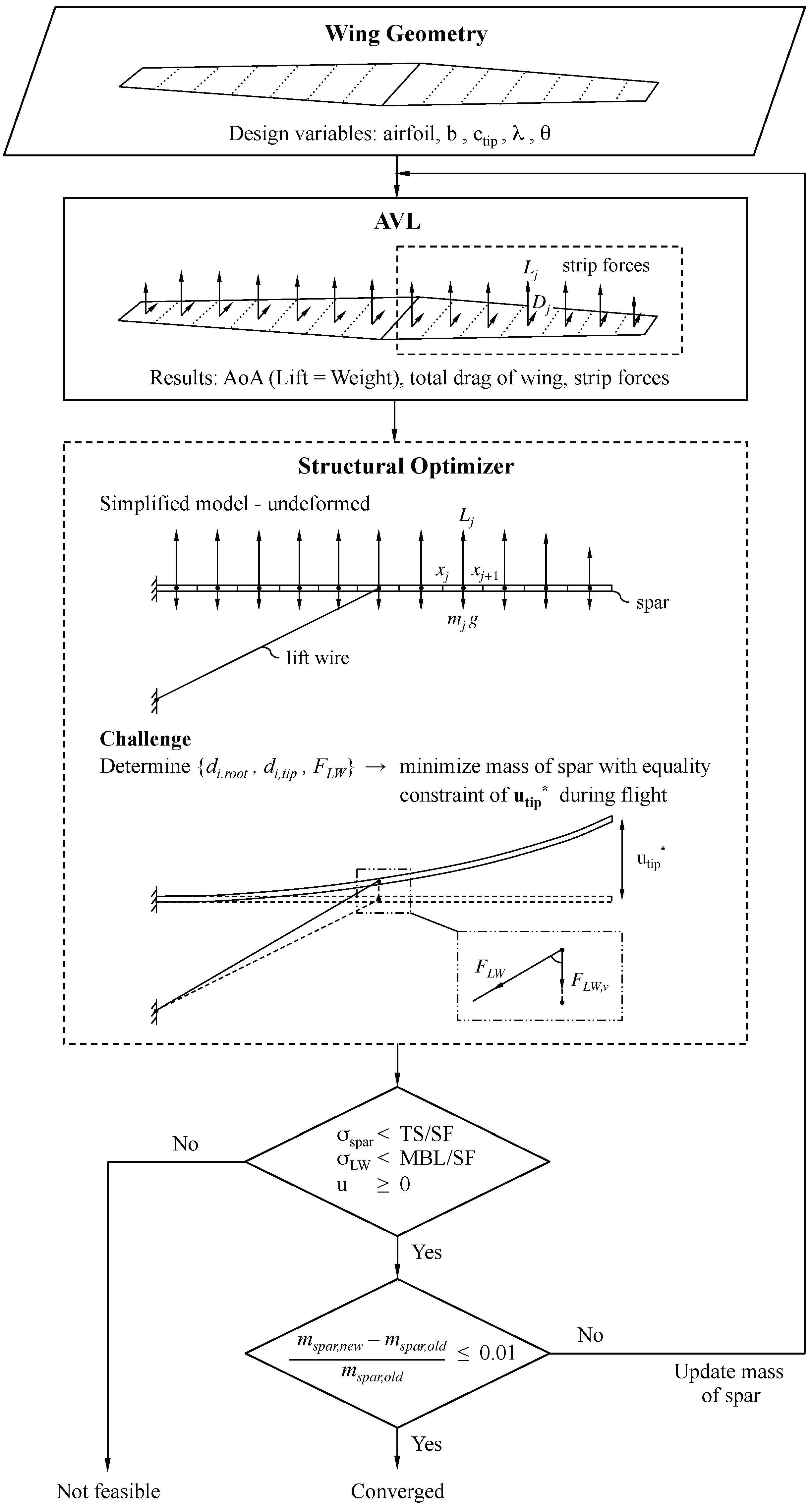
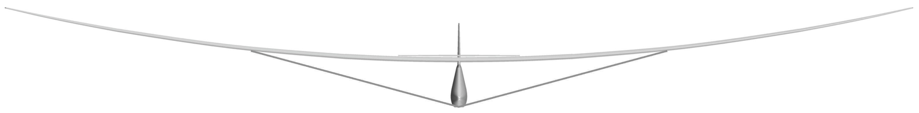
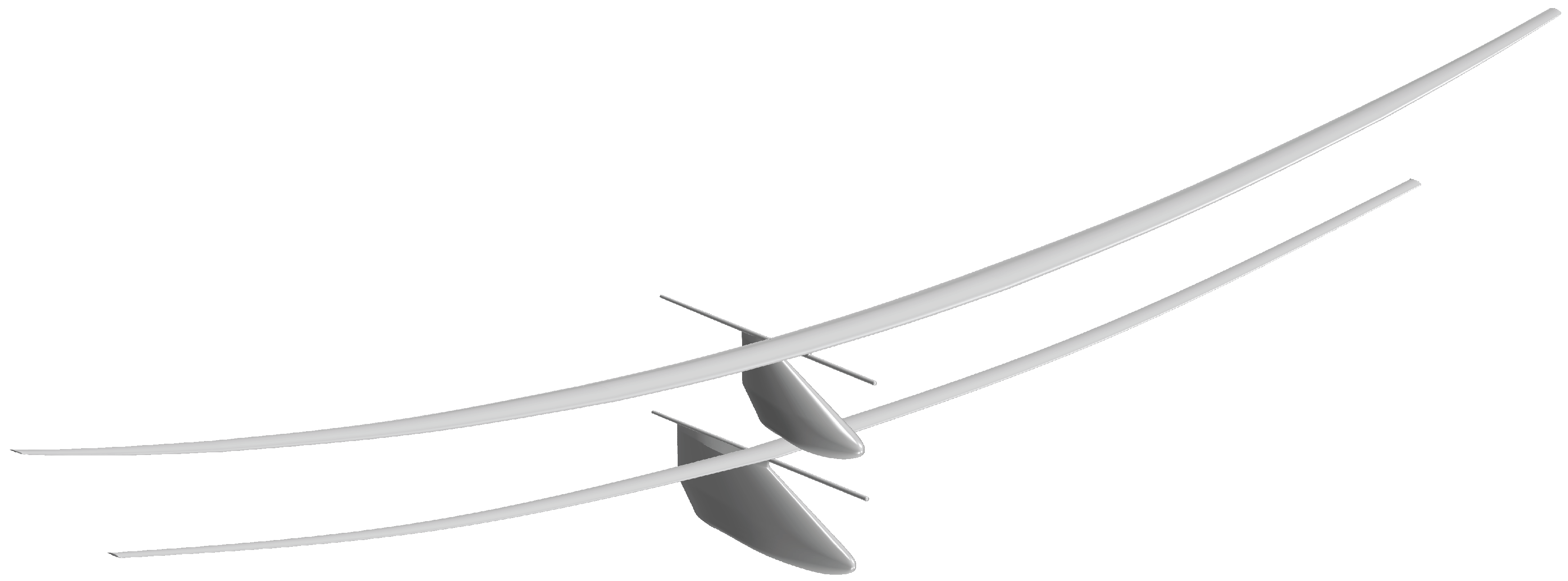
Knowing the forces acting on the undeformed wing from AVL, it is attempted to design the wing’s mechanical structure with the objective of minimizing the wing’s mass and an equality constraint to obtain a certain design tip deflection $u_{\mathrm{tip}}^{*}$. This design tip deflection is mostly determined from stability requirements. The wing’s mechanical structure is composed of two main parts. The first part is the wing’s internal structure, consisting of a spar and closely-spaced ribs. This internal structure is also the basis for the wing’s outer geometry, which is obtained by wrapping a Mylar sheet around the different ribs of the wing. The second mechanical structure is an external lift wire, which is basically a steel cable connected to the fuselage and the wing of the aircraft (Figure 11).

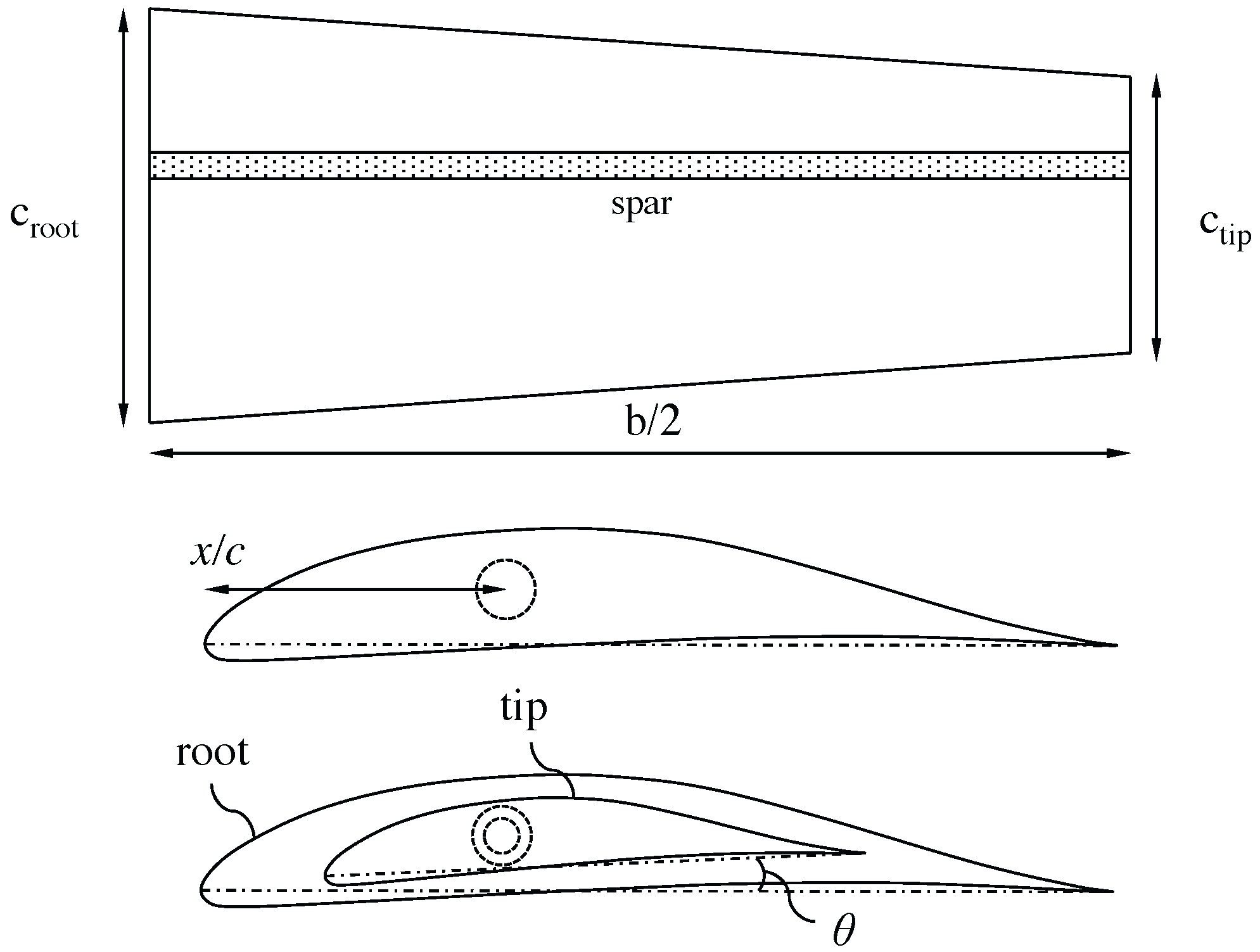
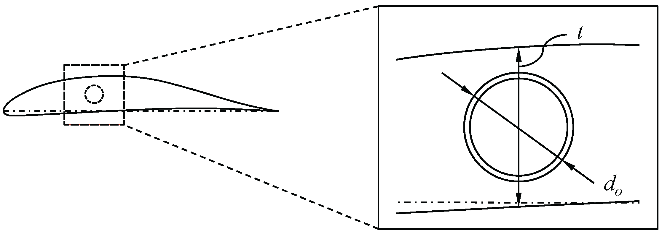
To guarantee that the spar will always fit into the wing, the design process is started by fixing the outer diameters of the spar geometrically. Based on the section’s local thickness t at the position of the spar (Figure 15), the outer diameters at the root and tip of the wing are taken as respectively 65% and 80% of the corresponding thickness. In addition, when the diameter at the root is found to be smaller than at the tip, e.g., when the wing is not tapered, both fractions are set to 65%. As such, the outer diameter at the root is always larger or equal to the outer diameter at the tip. It is now assumed that the outer diameters vary linearly from root to tip, which agrees with the linear variation of the chord lengths. At this point, the inner diameters of the spar are still unknown.

To determine the wing’s deflection during flight, the wing is represented by its spar and modeled as a cantilevered beam (Figure 13). The fixed and free end correspond to respectively the root and tip of the wing. Since the lift-to-drag ratio of the wing is usually very high for HPAs, being in the order of 45 for the Daedalus, only the vertical deformation due to the lift forces $L_j$ will be calculated here. When the wing deforms, the lift wire will exert an additional force $F_{\mathrm{LW}}$ onto the wing. However, this force can be adjusted by making the lift wire somewhat more loose or tight, and as such, this force is considered as an additional design variable.

The structural challenge now consists of finding a set of inner diameters of the wing’s spar at root and tip ($d_{i,\mathrm{root}}$, $d_{i,\mathrm{tip}}$) together with the force of the lift wire $F_{\mathrm{LW}}$, such that the wing experiences a certain design tip deflection $u_{\mathrm{tip}}^{*}$ during flight. Sequential Quadratic Programming (SQP) has been used for this optimization, and the optimizer runs until the relative change in the spar’s mass is less than 1%. As for the outer diameters of the spar, the inner diameters are assumed to vary linearly from root to tip. Further, it is attempted to minimize the mass of the wing’s spar while maintaining the design tip deflection.

To calculate the wing’s deflection for a certain set of inner diameters and force of the lift wire, the Euler–Bernoulli beam theory is applied and solved numerically using finite differencing. The equations are:

$$\begin{array}{cc}\hfill V_{j+1}-V_j& =f_j\hfill \\ \hfill M_{j+1}-M_j& =\left(\frac{V_{j+1}+V_j}{2}\right)(x_{j+1}-x_j)\hfill \\ \hfill {\theta }_{j+1}-{\theta }_j& =\left(\frac{{(M/EI)}_{j+1}+{(M/EI)}_j}{2}\right)(x_{j+1}-x_j)\hfill \\ \hfill u_{j+1}-u_j& =\left(\frac{{\theta }_{j+1}+{\theta }_j}{2}\right)(x_{j+1}-x_j)\hfill \end{array}$$

(3)

in which $f_j=L_j-m_{j}g$ and where V represents the shear force, M the bending moment, θ the deflection angle and u the deflection. The lift forces $L_j$ follow from the strip forces determined by AVL, and the masses $m_j$ follow from the inner and outer diameters of the spar and its material density. The force of the lift wire is included as follows:

$$x=b/4:f_j=L_j-m_{j}g-F_{\mathrm{LW},\mathrm{v}}$$

(4)

in which the lift wire is assumed to be connected underneath the fuselage and halfway between the root and tip of the wing. For the spar (a hollow tube), the second moment of area I is given by:

$$I=\frac{\pi }{64}(d_o^4-d_i^4)$$

(5)

and by specifying the Young’s modulus E, it is possible to determine the bending stiffness $EI$ in every discrete point $x_j$. Finally, the boundary conditions for the fixed and free end of the cantilevered beam can be expressed as:

$$\begin{array}{cccc}& x=0:\hfill & \hfill u& =0\hfill \\ & & \hfill \theta & =0\hfill \\ & x=b/2:\hfill & \hfill V& =0\hfill \\ & & \hfill M& =0.\hfill \end{array}$$

(6)

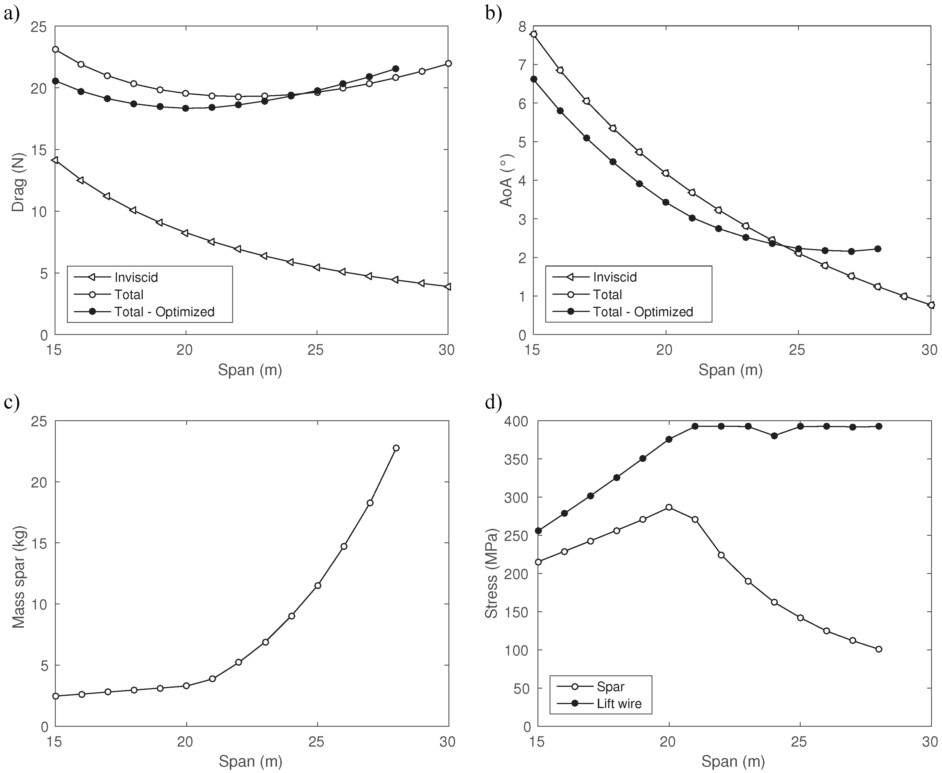
For each set of inner diameters and force of the lift wire considered during the structural optimization, a number of important conditions must be verified. First, the stresses occurring within the wing’s spar and lift wire should be below a certain maximal limit to avoid structural failure. For the spar, the maximal bending stress in every discrete point $x_j$ is given by:

$${\sigma }_j={\left(\frac{M{d}_o/2}{I}\right)}_j.$$

(7)

The shear stress will not be taken into account here, as its contribution was found to be negligible. For the lift wire, the tension is given by:

$${\sigma }_{\mathrm{LW}}=\frac{F_{\mathrm{LW}}}{A_{\mathrm{LW}}}$$

(8)

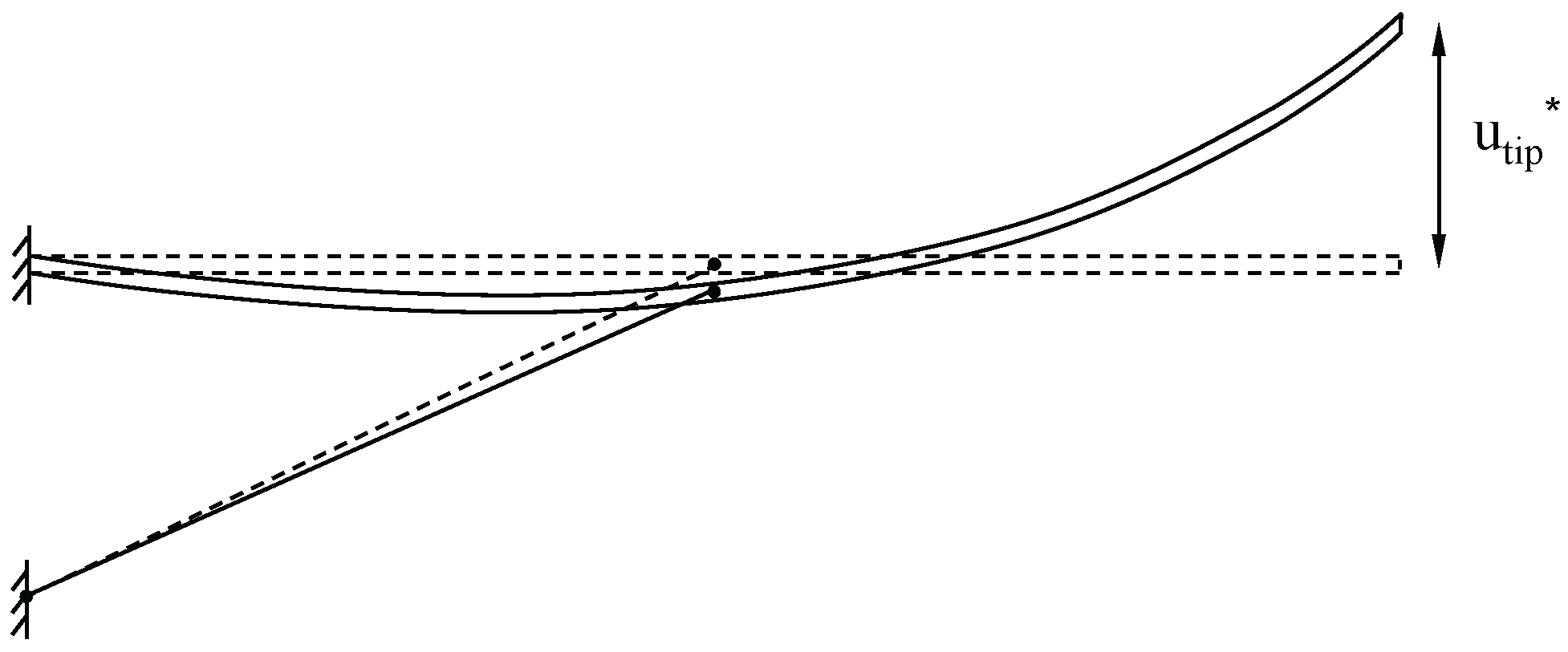
in which $A_{\mathrm{LW}}$ is the cross-sectional area of the lift wire. The material limits are indicated by the Tensile Strength (TS) in the case of the spar and by the Minimum Breaking Load (MBL) in the case of the lift wire. For both structures, an appropriate Safety Factor (SF) will be chosen. As a second condition, the deflection of the wing u may nowhere be negative. This second condition might need some further clarification. It is possible that the force exerted by the lift wire is so strong that the spar will deform negatively (downwards direction) near the root, but still achieves the desired tip deflection due to extreme bending towards the tip of the wing. Such a case is illustrated in Figure 16 and will not be considered as valid.

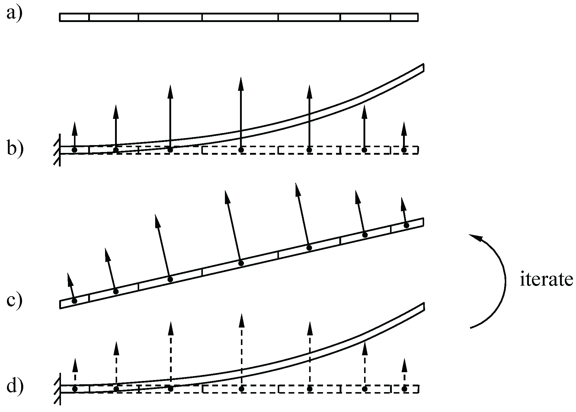
We remark that the final deformation of the wing is determined here using the forces acting on the undeformed wing. This approach is referred to as one-way aeroelastic. In order for the simulations to be FSI simulations, the deformed wing would have to be simulated again in AVL, and using the newly-determined strip forces, the deflection of the wing would have to be updated. This is repeated until the change between two consecutive iterations is found small enough. However, it will be shown in Section 5 that the one-way aeroelastic approach yields sufficiently accurate results compared to FSI, such that no coupling is required in the structural optimization.

To summarize, the structural optimization consists of finding a set of inner diameters and the force of the lift wire, such that the wing experiences a certain design tip deflection during flight. For the set to be feasible, the stresses occurring within the spar and lift wire should be limited, and the deflection should nowhere be negative. Further, it is attempted to find a feasible set that in addition minimizes the mass of the spar. This set is referred to as the optimal set.

4.4. Decision Blocks

If no set of inner diameters and force of the lift wire can be found that fulfills all constraints listed in the first decision block, the wing geometry is considered infeasible. If, on the other hand, an optimal set was found, the initial guess for the mass of the spar can be replaced by the correct mass, which is a function of the inner and outer diameters of the spar and its material density. The initial mass of the spar is taken as 8.62 kg, which corresponds with the spar of the Daedalus [1]. This update will change the mass of the aircraft structure and consequently the lift that has to be generated by the wing. This results in a slightly different angle of attack, drag of the wing and strip forces. The entire loop is repeated until the relative change in the spar’s mass is less than 1%. This complete optimization procedure was implemented in MATLAB.

4.5. Cases

As mentioned in the Introduction, it is intended to investigate if powering an HPA by two pilots offers some advantages. To do so, a separate wing will be designed for two cases; a single-pilot and a dual-pilot configuration.

Table 3. Design of experiments.

Property	Lower Boundary	Upper Boundary	Step Size
$x/c$	0.33	−	−
$\Gamma \left({}^{\circ }\right)$	6	−	−
b (m)	15	40	0.25
$c_{\mathrm{tip}}$ (m)	0.35	0.5	0.01
λ	0.25	1	0.01
$\theta {(}^{\circ })$	0	−	−

contains the lower and upper boundary of every geometrical design variable together with its step size, used to generate the large set of different wing geometries. The relative position $x/c$ of the spar’s center has been set to 0.33, and the desired tip deflection during flight is expressed via the dihedral angle Γ,

$$tan(\Gamma )=\frac{u_{\mathrm{tip}}}{b/2}$$

(9)

and as such, depends on the span b of the wing. The desired dihedral angle has been set to six degrees, which closely corresponds with the value of the Daedalus. Further, the twist angle was set to zero degrees, and 12 different airfoil types were investigated, in which each airfoil is specifically designed for HPAs or low-Reynolds number flows. The two pilots included in the optimization are not professional athletes, but rather two young engineering students whose masses are given in

Table 4. Structural properties of the spar and lift wire.

Property	Single-Pilot	Dual-Pilot
$m_{\mathrm{pilot}\left(\mathrm{s}\right)}$ (kg)	56.4	56.4 + 50.2
${\rho }_{\mathrm{spar}}$ (kg/m${}^3$)	1600	1600
$E_{\mathrm{spar}}$ (GPa)	200	200
$T{S}_{\mathrm{spar}}$ (MPa)	1600	1600
$S{F}_{\mathrm{spar}}$	4	4
$MB{L}_{\mathrm{LW}}$ (MPa)	1570	1570
$S{F}_{\mathrm{LW}}$	4	4
$d_{\mathrm{LW}}$ (mm)	18	25

. The table further contains the structural properties of the spar and lift wire, in which the spar is constructed from high modulus carbon fiber with a minimal wall thickness of 0.8 mm and where the lift wire is a stainless steel wire rope. For both structures, the Safety Factor (SF) was set to four. Finally, note that a different diameter of the lift wire is used in the dual-pilot configuration.

5. Fluid–Structure Interaction (FSI) Simulation

It was stated that the one-way aeroelastic approach to determine the final deformation of the wing yields sufficiently accurate results compared to FSI. To prove this statement, an example FSI simulation will be performed in this section. For a better understanding, the FSI procedure (Figure 17) is first explained in some more detail. The use of a lift wire will not be considered here. Starting from a perfectly straight wing (Figure 17a) and a set of flight conditions (velocity and lift), AVL will determine the wing’s angle of attack, drag and strip forces. The strip forces are given to MATLAB, which will determine the deflection of the wing using the finite differencing method (Figure 17b). The geometry of the wing can now be updated, but since only two sections (root and tip) are used to define the wing geometry, the actual deflection is simplified by a linear deflection in which the tip deflection is identical. This deformed wing geometry is then simulated back again in AVL, resulting in a new angle of attack, drag and strip forces (Figure 17c). To calculate the new deflection of the wing, the vertical components of the strip forces are determined and applied to the undeformed wing (Figure 17d). As such, the sum of the forces in Figure 17d is equal to the specified lift needed to carry the pilot and the aircraft structure. The deflection can now be determined, allowing one to update the wing geometry once more. This procedure is repeated until the relative change of the wing geometry is found small enough.

For the intended FSI simulation, the geometrical and structural data of the wing are given in

Table 5. Geometrical and structural properties in the Fluid–Structure Interaction (FSI) simulation.

Geometrical		Structural
b	20 m	$m_{\mathrm{pilot}}$	56.4 kg
$c_{\mathrm{tip}}$	0.5 m	$m_{\mathrm{aircraft}}$	30.6 kg
λ	0.5	${\rho }_{\mathrm{spar}}$	1600 kg/m${}^3$
θ	0 ${}^{\circ }$	$E_{\mathrm{spar}}$	200 GPa

. The airfoil used to construct the wing is the DAE11, and the wall thickness of the spar $t_{\mathrm{spar}}$ is set to 1 mm. Recall that the outer diameters of the spar are fixed for the given wing geometry. Further, the flight velocity is set to 12 m/s.

The results of the FSI simulation are provided in

Table 6. Results of an example FSI simulation.

Iteration	L (N)	${\mathit{u}}_{\mathit{tip}}$ (m)	$\mathbf{\Gamma }{(}^{\mathbf{\circ }})$	${\mathit{\sigma }}_{\mathit{max}}$ (MPa)	${\mathit{\tau }}_{\mathit{max}}$ (MPa)
0	426.72	1.1720	6.6843	324.38	3.05
1	426.70	1.1694	6.6699	323.77	3.04
2	426.70	1.1694	6.6701	323.78	3.04
3	426.70	1.1694	6.6701	323.78	3.04
4	426.70	1.1694	6.6701	323.78	3.04
5	426.70	1.1694	6.6701	323.78	3.04

. The relative change in tip deflection $u_{\mathrm{tip}}$ after the first iteration is found to be 0.2%. As such, no iterations are actually required to determine the final deflection of the wing, which confirms the above statement. Table 6 also contains the maximal bending stress ${\sigma }_{max}$ and shear stress ${\tau }_{max}$ occurring in the spar. As mentioned, the contribution of the shear stress is indeed negligible.

The one-way aeroelastic approach could also be called a single Gauss–Seidel coupling iteration between the flow calculation and the structural calculation. As the tip deflection changed only 0.2% after the first iteration (Table 6) in the FSI simulation, the significant additional cost of multiple Gauss–Seidel iterations is not justified, and only one iteration is most appropriate, meaning that the structural deformation is not affecting the flow calculation.

6. Sensitivity Study

The purpose of the following sensitivity studies is to investigate the influence of every geometric design variable separately.

Table 7. Overview of the sensitivity studies. An asterisk * indicates the desired value during flight.

Property	Study 1	Study 2	Study 3	Study 4	Study 5
Airfoil	DAE11	DAE11	DAE11	DAE11	DAE11
$x/c$	0.33	0.33	0.33	0.33	0.33
$\Gamma {(}^{\circ })$	0–10	6*	6*	6*	6*
b (m)	20	15–30	20	20	20
$c_{\mathrm{tip}}$ (m)	0.5	0.5	0.35–0.75	0.5	0.5
λ	1	1	0.5	0.25–1	1
$\theta {(}^{\circ })$	0	0	0	0	0–5

gives an overview of the different studies in which the values indicated with an asterisk correspond to the desired value during flight. The flight velocity is set to 12 m/s, and the structural properties of the spar and lift wire are identical to the values listed in Table 4 for the single-pilot case.

In most of the studies, every wing geometry will be analyzed in three different ways. This is started by performing an inviscid and viscous analysis of the wing in its undeformed state in AVL, in which the corresponding induced and total drag is calculated. Further, the wing geometry will be structurally optimized (if possible) for a certain design dihedral angle during flight. The results of Studies 2 and 5 will be analyzed in great detail, whereas Studies 1, 3 and 4 will only be briefly discussed.

6.1. Study 1: Dihedral Angle

In the first study, it is proven that the dihedral angle Γ has almost no influence on the aerodynamic performance of the wing (Figure 18). As mentioned, the desired dihedral angle during flight is actually determined from stability requirements, more specifically the roll stability. The design value has been set to six degrees in this work, similar to the Daedalus, but note that the value during flight can still be adjusted later on by making the lift wires somewhat more tight or loose compared to the design setting. Given the safety factor of four for the maximal material stresses in the spar and lift wire, this adjustment should be allowable.

6.2. Study 2: Wing Span

In the second study, the span of the wing b is increased from 15 to 30 m in steps of 1 m. Increasing the span of the wing is found to be beneficial for decreasing the induced drag of the wing (Figure 19a). However, as the span increases, the surface area of the wing increases, causing additional viscous drag. As such, the total drag of the wing will exhibit a minimum for a certain wing span, in this case around 22 m. Every wing geometry of this study is now structurally optimized. The mass of the spar as a function of the span can be seen in Figure 19c, and Figure 19d shows the corresponding maximal stress occurring in the spar and lift wire. For a wing span up to 24 m, the spar can be made lighter than initially assumed. Recall that the initial mass of the spar was taken as 8.62 $\mathrm{k}\mathrm{g}$, corresponding to the spar of the Daedalus. The result is a lighter aircraft structure, such that the wing must generate less lift. This is accomplished by decreasing the angle of attack compared to the unoptimized wing (Figure 19b) and is seen to reduce the total drag of the wing. The lift wire reaches its full potential at a wing span of around 21 m. To limit the tip deflection for a larger span, this can now only be accomplished by making the spar itself stiffer. This is done by increasing its wall thicknesses, resulting in a heavier spar, but lower bending stresses. For a wing span larger than 28 m, the wing geometries are found infeasible.

6.3. Studies 3 and 4: Tip Chord Length and Taper Ratio

The most important results of the third and fourth study are that the total drag of the wing continuously decreases with decreasing tip chord length (Figure 20a) and that the point of minimal drag is very weak in the case of the taper ratio (Figure 20b).

6.4. Study 5: Twist Angle

In the final study, the twist angle θ is increased from zero to five degrees in steps of 0.5 degrees. Note that increasing the twist angle causes the incidence of the tip profile to be smaller than the root profile (Figure 14). Compared to the case of no twist, the wing will generate less lift, which is compensated by increasing its angle of attack (Figure 21b). Although the angle of attack of the complete wing has increased, the local angle of attack near the tip has decreased, since the slope in Figure 21b is smaller than one. As such, less lift is being generated near the tip, resulting in lower bending moments and stresses (Figure 21d). Note that the angle of attack of the structurally-optimized wing geometries is smaller compared to the unoptimized designs. This is due to the lower mass of the spar, resulting in a lighter aircraft structure and less required lift. As the loading is smaller near the tip, the tip deflection will also be smaller, such that the stress in the lift wire is seen to decrease. The influence on the total drag of the wing is found to be small, but twisting the wing is slightly advantageous up to a twist angle of three degrees (Figure 21a).

7. Optimization: Results

As outlined in Section 4, a large set of different wing geometries was generated and individually structurally optimized for two cases. The structural optimization of one specific wing geometry took about 8 to 15 s and mostly required two to six iterations. For each case and airfoil type, the geometrical and structural data of the optimal wing design is given in

Table 8. Geometrical and structural data of optimal designs (upper table: single-pilot; lower table: dual-pilot). The line in bold indicates the design which requires the lowest power per pilot.

Single-Pilot	b	${\mathit{c}}_{\mathit{tip}}$	λ	Γ	${\mathit{t}}_{\mathit{root}}$	${\mathit{t}}_{\mathit{tip}}$	${\mathit{m}}_{\mathit{spar}}$	${\mathit{\sigma }}_{\mathit{spar}}$	${\mathit{\sigma }}_{\mathit{LW}}$	$\mathit{AoA}$	D	$\mathit{P}/\mathit{pilot}$
Airfoil	(m)	(m)	−	(°)	(mm)	(mm)	(kg)	(MPa)	(MPa)	(°)	(N)	(W)
DAE11	20.75	0.35	0.58	6	0.80	0.80	3.53	249	334	3.38	16.85	202
DAE21	21.00	0.35	0.58	6	0.81	0.81	3.31	298	367	3.11	15.58	187
DAE31	20.25	0.35	0.62	6	1.09	1.09	3.83	274	359	3.20	15.22	183
E395	22.00	0.35	0.64	6	1.00	1.00	4.18	273	388	2.21	14.18	170
E396	22.50	0.35	0.62	6	0.81	0.81	3.77	287	392	1.79	14.62	175
E397	22.75	0.35	0.63	6	0.80	0.80	3.89	277	391	1.92	14.92	179
E398	23.25	0.35	0.64	6	0.80	0.80	4.13	264	392	1.95	15.05	181
E399	23.50	0.35	0.66	6	0.80	0.80	4.30	252	391	2.00	15.44	185
FX63-137	23.50	0.35	0.60	6	0.80	0.80	4.18	264	392	-0.49	14.65	176
FX76MP120	18.75	0.35	0.70	6	0.89	0.89	3.00	295	342	1.35	17.10	205
FX76MP140	19.50	0.35	0.70	6	0.80	0.80	3.28	250	329	-2.22	17.15	206
L7769	20.25	0.35	0.58	6	0.98	0.98	3.52	285	355	7.00	16.93	203
Dual-Pilot	$\mathit{b}$	${\mathit{c}}_{\mathit{tip}}$	λ	Γ	${\mathit{t}}_{\mathit{root}}$	${\mathit{t}}_{\mathit{tip}}$	${\mathit{m}}_{\mathit{spar}}$	${\mathit{\sigma }}_{\mathit{spar}}$	${\mathit{\sigma }}_{\mathit{LW}}$	$\mathit{AoA}$	$\mathit{D}$	$\mathit{P}/\mathit{pilot}$
Airfoil	(m)	(m)	−	(°)	(mm)	(mm)	(kg)	(MPa)	(MPa)	(°)	(N)	(W)
DAE11	27.50	0.35	0.47	6	1.21	1.21	8.01	284	388	4.50	25.72	154
DAE21	27.75	0.35	0.46	6	1.62	1.62	9.94	255	392	4.27	24.15	145
DAE31	27.25	0.35	0.46	6	1.89	1.89	10.52	253	392	3.79	23.42	141
E395	28.75	0.35	0.46	6	1.65	1.65	10.94	239	388	2.88	22.47	135
E396	28.75	0.35	0.46	6	1.36	1.36	9.68	250	392	2.79	23.04	138
E397	28.50	0.35	0.48	6	1.32	1.32	9.38	253	392	3.27	23.35	140
E398	29.25	0.35	0.47	6	1.20	1.20	9.32	250	392	2.98	23.86	143
E399	28.75	0.35	0.46	6	0.90	0.90	7.33	284	392	2.86	24.26	146
FX63-137	29.50	0.35	0.42	6	1.03	1.03	8.38	265	392	0.12	23.35	140
FX76MP120	26.25	0.35	0.55	6	1.93	1.93	10.20	255	392	2.17	24.99	150
FX76MP140	27.00	0.35	0.57	6	1.46	1.46	9.22	258	392	-1.17	24.75	149
L7769	27.25	0.35	0.43	6	1.64	1.64	9.45	266	391	7.49	26.72	160

. In every optimal design, the wing is found to be tapered in which the tip chord length corresponds to its lower boundary. This result is in agreement with the observations made in the sensitivity study (Figure 20a). The wings are somewhat more tapered in the dual-pilot case, the taper ratio λ being smaller compared to the single-pilot case. Comparing the optimal designs of the single- and dual-pilot case with the same airfoil, the higher lift needed in the dual-pilot configuration results in a larger span b, a larger angle of attack AoA and a heavier spar. The wall thicknesses of the spar at root and tip ($t_{\mathrm{root}}$, $t_{\mathrm{tip}}$) are also given and found to be identical in each optimal wing design. Recall that the outer diameters of the spar are geometrically fixed, such that the wall thicknesses allow one to calculate the spar’s inner diameters. Further, every design makes use of a lift wire (LW) in which the lift wires are mostly exploited to their maximum allowable stress. The maximal stress occurring in the spar (${\sigma }_{\mathrm{spar}}$) is seen to be comparable in both cases. However, the most interesting result is the drag of the wing D. Although the drag is seen to be larger in the dual-pilot cases, when dividing the corresponding required power over two pilots, there clearly seems to be an advantage. The reduction in the required power per pilot is found to range from 35 to 57 $\mathrm{W}$. The most optimal wing is thus found to be for two pilots. Comparing the results for the different airfoils in the dual-pilot case, the E395 is seen to be the most optimal. Using this most optimal wing, our HPA will now be further constructed and designed for two pilots.

Complete Optimized Design

The idea consists of taking the Daedalus and replacing its wing by our own optimized wing and to adjust its fuselage to fit a second pilot. The incidence of the wing with respect to the aircraft is taken as the angle of attack determined in Table 8. The optimized wing was further given a twist of one degree, found to slightly increase its performance (Figure 21). The fuselage was extended by 1.5 m, assuring sufficient space for the second pilot. Concerning the stability, both the Daedalus and our optimized design were found to be statically stable in AVL. The CAD model of the wing and fuselage of our optimized design is shown in Figure 22 together with the Daedalus for comparison.

The optimized design was also simulated in STAR-CCM+, being the final simulation. As for the Daedalus, the CFD simulation was performed steadily, in which the flight velocity was set to 12 m/s and the angle of attack of the aircraft to 1.30 degrees. The results of the CFD simulation are given in

Table 9. Comparison Daedalus versus optimized design in STAR-CCM+.

Property	Daedalus	Optimized
Total Mass (kg)	105.4	147.0
Flight Velocity (m/s)	6.7	12
AoA Aircraft (${}^{\circ }$)	2.76	1.30
Gliding Drag (N)	26.2	32.3
Wing (N)	23.67	22.76
Fuselage (N)	1.05	4.24
Elevator (N)	0.44	2.36
Rudder (N)	0.53	1.60
Tail Boom (N)	0.47	1.32
Lift (N)	1034.8	1465.5
Propulsive Efficiency	0.90	0.90
Total Power (W)	195	430
Pilot Power (W)	195	215

and are compared with the CFD results of the Daedalus. Therefore, in the case of our optimized design, each pilot should generate a power of 215 W in order to obtain a flight velocity of 12 m/s. Note that this flight velocity is 80% higher compared to the Daedalus, while the corresponding pilot power has only increased by 10%. An interesting result is that the total drag of the optimized wing is smaller compared to the Daedalus. However, the parasite drag has substantially increased. The drag of the fuselage has increased with a factor four, which is due to the higher frictional surface. Further, note that the generated lift is somewhat larger than the total weight, which is a small safety and allows one to carry an additional 2.4 kg. The final step consists of measuring the physical performance of our two pilots.

8. Final Test

The physical performance was measured using a bicycle trainer with an adaptive resistive power. Starting at a low resistive power of 60 W, the power was gradually increased every 2 min by 20 W until the pilot reached total fatigue. The results of the power test are shown in Figure 23, in which the Heart Rates (HR) of both pilots are given as a function of time together with the resistive power. Pilot 1 is seen to produce a maximal power output of 260 W, compared to 240 W for Pilot 2. As such, the pilots can produce a peak power output of 500 W, which is definitely larger than the theoretical power of 430 W needed to obtain a flight velocity of 12 m/s. However, in order to win the Kremer International Marathon Competition, the pilots must sustain the aircraft at this 12 m/s during 1 h. Dividing the theoretical required power over the two pilots based on their maximal power output results in respectively 223.6 W for Pilot 1 and 206.4 W for Pilot 2. These values correspond with 86% of their maximal physical performance.

9. Conclusions

The goal of this work was to design and optimize an HPA capable of winning the Kremer International Marathon Competition. As a first step, it was investigated how accurately the required pilot power to fly an HPA could be predicted. This was done by simulating an existing design (the Daedalus) in two different software; AVL (vortex lattice method) and STAR-CCM+ (computational fluid dynamics). In AVL, the pilot power was underpredicted by about 18% compared to the value provided by MIT, but the required computational time was only in the order of seconds. This very short calculation time made AVL an ideal tool for the optimization of our own HPA. For the simulation in STAR-CCM+, a preliminary two-dimensional CFD study of the airfoil FX63-137 was performed first. The study clearly showed the need of a transition model, in this case the γ-Re${}_{\theta }$ transition model, in order to obtain accurate drag predictions at low Reynolds numbers. The predicted pilot power in STAR-CCM+ was found to agree within 3%, but the simulation required a large amount of computational power and time.

As a second step, a new HPA was designed and optimized for the Kremer International Marathon Competition. It was started by optimizing a wing on itself, in which a large set of different wing geometries was generated and individually structurally optimized for two cases; a single-pilot and dual-pilot configuration. The structural optimization consisted of finding a set of inner diameters of the wing’s spar at root and tip and the force of the lift wire, minimizing the wing’s mass while obtaining a certain design tip deflection during flight. From this large set, the optimal wing was taken as the wing geometry with the lowest total drag and that was structurally feasible. An interesting result was that adding a second pilot on board of the aircraft was found to be beneficial, the reduction in required pilot power ranging from 35 to 57 W. Based on the design of the Daedalus and our own optimized wing, a complete HPA was constructed for two pilots. The optimized design was simulated in STAR-CCM+ resulting in a theoretical required power of 430 W in order to obtain the design flight velocity of 12 m/s.

As a final step, the physical performance of two candidate pilots was measured. Together, they were able to produce a peak power output of 500 W, being largely sufficient to reach the design flight velocity for a short period of time. However, to win the Kremer International Marathon Competition, both pilots must theoretically produce 86% of their maximal physical performance during one hour. With some further optimization and the design of a propeller and the aircraft’s steering, completing the marathon course within time does not seem impossible. Constructing our optimized HPA and attempting the Kremer International Marathon Competition could be a next step.

References

1. McIntyre, J. Man’s Greatest Flight. AeroModeller. 1988. Available online: http://library.propdesigner.co.uk/daedalus.pdf (accessed on 1 May 2016).
2. AVL (Athena Vortex Lattice). Available online: http://web.mit.edu/drela/Public/web/avl/ (accessed on 1 May 2016).
3. Regulations and Conditions for the Kremer International Marathon Competition. Available online: http://aerosociety.com/About-Us/specgroups/Human-Powered/Kremer (accessed on 1 May 2016).
4. Fazzolari, A.; Gauger, N.R.; Brezillon, J. Efficient aerodynamic shape optimization in MDO context. J. Comput. Appl. Math. 2007, 203, 548–560. [Google Scholar] [CrossRef]
5. Kenway, G.K.W.; Kennedy, G.J.; Martins, J.R.R.A. Scalable Parallel Approach for High-Fidelity Steady-State Aeroelastic Analysis and Adjoint Derivative Computations. AIAA J. 2014, 52, 935–951. [Google Scholar] [CrossRef]
6. Tang, D.; Dowell, E.H. Experimental Aeroelastic Models Design and Wind Tunnel Testing for Correlation with New Theory. Aerospace 2016, 3, 12. [Google Scholar] [CrossRef]
7. Guo, S.; De Los Monteros, J.E.; Liu, Y. Gust Alleviation of a Large Aircraft with a Passive Twist Wingtip. Aerospace 2015, 2, 135–154. [Google Scholar] [CrossRef]
8. ASWING: Configuration Development System for Flexible Aircraft. Available online: http://web.mit.edu/drela/Public/web/aswing/ (accessed on 1 May 2016).
9. Drela, M. Low-Reynolds-Number Airfoil Design for the MIT Daedalus Prototype: A Case Study. J. Aircr. 1988, 25, 724–732. [Google Scholar] [CrossRef]
10. Cruz, J.R.; Drela, M. Structural Design Conditions for Human Powered Aircraft. In Proceedings of the 21st OSTIV Conference, Wiener Neustadt, Austria, 1989.
11. Katz, J.; Plotkin, A. Low-Speed Aerodynamics, 2nd ed.; Cambridge University Press: New York, NY, USA, 2001. [Google Scholar]
12. XFOIL: Subsonic Airfoil Development System. Available online: http://web.mit.edu/drela/Public/web/xfoil/ (accessed on 1 May 2016).
13. Hansen, T. Modeling the Performance of the Standard Cirrus Glider using Navier-Stokes CFD. Tech. Soar. 2014, 38, 5–14. [Google Scholar]
14. Morgado, J.; Vizinho, R.; Silvestre, M.A.R.; Páscoa, J.C. XFOIL vs. CFD performance predictions for high lift low Reynolds number airfoils. Aerosp. Sci. Technol. 2016, 52, 207–214. [Google Scholar] [CrossRef]
15. Drela, M. Aerodynamics of Human-Powered Flight. Annu. Rev. Fluid Mech. 1990, 22, 93–110. [Google Scholar] [CrossRef]
Figure 1. The Daedalus.
Aerospace 03 00026 g001
Figure 2. The Kremer International Marathon Competition.
Aerospace 03 00026 g002
Figure 3. CAD model of the Daedalus.
Aerospace 03 00026 g003
Figure 4. AVL model of the Daedalus plotted on top of its CAD model.
Aerospace 03 00026 g004
Figure 5. Drag polar of DAE11 at a Reynolds number of 500,000.
Aerospace 03 00026 g005
Figure 6. Laminar separation bubble [13].
Aerospace 03 00026 g006
Figure 7. 2D section of the trimmed hexahedral mesh (FX63-137).
Aerospace 03 00026 g007
Figure 8. Trimmed hexahedral mesh around the Daedalus.
Aerospace 03 00026 g008
Figure 9. Two-dimensional results of the airfoil FX63-137: (a) lift coefficient versus angle of attack; (b) drag coefficient versus angle of attack; (c) drag polar; (d) lift-to-drag ratio versus angle of attack.
Aerospace 03 00026 g009
Figure 10. Two-dimensional results of the airfoil FX63-137: (a) pressure coefficient distribution at zero degrees angle of attack; (b) comparison of turbulent kinetic energy (upper airfoil: computational fluid dynamics (CFD) without transition; lower airfoil: CFD with transition).
Aerospace 03 00026 g010
Figure 11. Lift wires of the Daedalus.
Aerospace 03 00026 g011
Figure 12. Transition from laminar to turbulent flow on the Daedalus visualized by the constrained streamlines and the turbulent kinetic energy.
Aerospace 03 00026 g012
Figure 13. Structural optimization procedure.
Aerospace 03 00026 g013
Figure 14. Parameterized wing geometry.
Aerospace 03 00026 g014
Figure 15. Defining the spar’s outer diameters.
Aerospace 03 00026 g015
Figure 16. Invalid design with negative deflection near the root.
Aerospace 03 00026 g016
Figure 17. Fluid–Structure Interaction (FSI) procedure: (a) Initial geometry for AVL; (b) deflection of the wing based on the initial forces from AVL; (c) deflected geometry for AVL with linear variation of the deflection along the span; (d) deflection of the wing based on the updated forces from AVL.
Aerospace 03 00026 g017
Figure 18. Sensitivity study: dihedral angle.
Aerospace 03 00026 g018
Figure 19. Sensitivity study: wing span. (a) Drag; (b) angle of attack; (c) mass of the spar; (d) maximal stress.
Aerospace 03 00026 g019
Figure 20. Sensitivity study: (a) tip chord length; (b) taper ratio.
Aerospace 03 00026 g020
Figure 21. Sensitivity study: twist angle. (a) Drag; (b) angle of attack; (c) mass of the spar; (d) maximal stress.
Aerospace 03 00026 g021
Figure 22. Comparison of wing and fuselage (upper: Daedalus; lower: optimized dual-Human-Powered Aircraft (HPA)).
Aerospace 03 00026 g022
Figure 23. Power test of the pilots.
Aerospace 03 00026 g023