Ushering in the New Era of Radiometric Intercomparison of Multispectral Sensors with Precision SNO Analysis

Abstract

A “nadir-only” framework of the radiometric intercomparison of multispectral sensors using simultaneous nadir overpasses (SNOs) is examined at the 1-km regimes and below using four polar-orbiting multispectral sensors: the twin MODerate-resolution Imaging Spectroradiometer (MODIS) in the Terra and Aqua satellites, the Visible Imaging Infrared Radiometer Suite (VIIRS) in the Suomi National Polar-orbiting Partnership (SNPP) satellite, and the Ocean and Land Colour Instrument (OLCI) in the Sentinel-3A satellite. The study is carried out in the context of isolating the on-orbit calibration of the reflective solar bands (RSBs) under the “nadir-only” restriction. With a homogeneity-ranked, sample size constrained procedure designed to minimize scene-based variability and noise, the overall approach successfully stabilizes the radiometric ratio and tightens the precision of each SNO-generated comparison event. Improvements to the multiyear comparison time series are demonstrated for different conditions of area size, sample size, and other refinements. The time series demonstrate the capability at 1% precision or better under general conditions but can attain as low as 0.2% in best cases. Solar zenith angle is examined not to be important in the “nadir-only” framework, but the spectral mismatch between two bands can give rise to significant yearly modulation in the comparison time series. A broad-scaled scene-based variability of ~2%, the “scaling phenomenon”, is shown to have pervasive presence in both northern and the southern polar regions to impact inter-RSB comparison. Finally, this paper highlights the multi-instrument cross-comparisons that are certain to take on a more important role in the coming era of high-performing multispectral instruments.

1. Introduction

Earth science and climate studies have made significant progress in the recent decades along with continual advances in remote sensing technologies. Progressing along improving imaging capability is the intersensor comparison methodology, a method of evaluating the performance of sensor data or associated retrievals by comparing against a reference sensor, which is also certain to be utilized in greater capacity in the coming era. For multispectral sensors, it can be argued that the two units of the MODerate-resolution Imaging Spectradiometer (MODIS) [1,2], in the Terra and Aqua satellites launched on 18 December 1999 and 4 May 2002, respectively, are the forerunners leading the era of the high-performance instruments and big data. The twin MODIS, with 36 bands covering the spectral range of 0.45 to 12.4 μm are now closing in on two prolific decades of data acquisition. However, it is not until the launch of the next major multispectral sensor—the Visible Imaging Infrared Radiometer Suite (VIIRS) aboard the Suomi National Polar-orbiting Partnership (SNPP) satellite on 28 October 2011 [3,4]—that the twin MODIS finally has a comparable counterpart to generate high precision intersensor comparison result. Numerous radiometric intercomparisons of the reflective solar bands (RSBs) of Aqua MODIS and SNPP VIIRS ensued [5,6,7] utilizing the simultaneous nadir overpasses (SNOs) approach [8,9,10,11]. These studies demonstrated the capability of the radiometric intercomparison at the 1-km spatial resolution regime to be typically few percent. A main goal of this paper is to show that the capability, under an improved analysis procedure, is at the level of 1% precision or better.

The coming era is certain to make intersensor comparison a tool of increasing importance as more high-performance multispectral sensors are continually being launched into operation. For example, the Ocean and Land Colour (OLCI) Instrument and its companion Sea and Land Surface Temperature Radiometer (SLSTR) housed in the Sentinel-3A satellite [12] are the recently launched polar-orbiting multispectral sensors, with approximately 300-m spatial resolution. The first follow-on of VIIRS built is one on the Joint Polar Satellite System-1 (JPSS-1) satellite [13], or J1 satellite (officially designated as NOAA-20 post launch), was launched on 18 November 2017. A total of four follow-on VIIRS—J1 to J4 VIIRS—for which the SNPP VIIRS serves as the precursor, are scheduled to span the next 20 years of operation. The technological advancement also extends to geostationary sensors, with Himawari-8 Advanced Himawari Imager (AHI) [14,15], GOES-R Advanced Baseline Imager (ABI) [16,17,18], and GOES-S ABI [18], all with 1-km spatial resolution, recently launched. More follow-on geostationary sensors are also in the plan of succession. The demand for assessing sensor data quality and to monitor radiometric performance will certainly increase.

The overall accuracy of radiometric data depends on many inputs, but the regularly carried out on-orbit radiometric calibration operation to characterize the changing performance of detectors is one of central importance. One main commonality among the four instruments considered here—Terra and Aqua MODIS, SNPP VIIRS, and Sentinel-3A OLCI—is a fully equipped onboard calibration suite for carrying out the regularly scheduled on-orbit calibration. They following a similar strategy, including using a specially made solar diffuser (SD) panel for RSB performance characterization. This built-in calibration capability is a mark of the new generation high-performance multispectral sensors and makes them valuable radiometric references for other sensors or any climate studies to inter- or cross-calibrate. Thus establishing radiometric consistency between any pair of such independently calibrated sensor will be beneficial, and intersensor comparison is a most proper tool for this purpose. In addition, intercalibration using any of these sensors as a radiometric reference requires also a reliable intersensor comparison methodology. While there are numerous approaches for post-launch radiometric evaluation, the current knowledge points to intersensor comparison as potentially the most precise approach.

However, there are many other factors impacting the overall accuracy of the sensor data and also intersensor comparison result beyond just band or detector performance. One of such, outside the capability of the standard on-orbit calibration, is the response-versus-scan angle (RVS) effect of the scan mirror that can add in a systematic angle-dependent bias along-scan. For example, in the MODIS Collection 6 release [19,20], the addition of the time-dependent RVS characterization is a key upgrade to the RSB calibration methodology to mitigate the RVS effect that is beyond the capability of the on-orbit calibration methodology. For SNPP VIIRS, the time-dependent RVS effect is not yet an issue, but its potential emergence remains a possibility. Various common issues also create challenges for intersensor comparison analysis. Angle- or scene-dependent effects associated with the scenes, including the biredirectional reflectance distribution factor (BRDF) of the SNO scenes, also introduce additional complications into intersensor comparison result. For removing various confounding effects associated with larger angles or viewing areas, Chu et al. [7] utilized a “nadir-only” framework of SNO analysis in an Aqua MODIS versus SNPP VIIRS study, that limits the viewing angle to the Earth scenes to near 0° degree by using a small-sized comparison area. This study adopts the same “nadir-only” approach specifically in the context of examining the capability of intercomparison in evaluating on-orbit RSB calibration performance, and furthermore uses multiyear comparison time series that incorporate all high-quality SNO events as a tool of evaluation.

This study further distinguishes between statistical and physical constraints. For example, statistical analyses subject all physical conditions such as cloudy scenes or those of various geolocational conditions under the same criteria. This analysis carefully avoids any premature applications of physical constraints, such as the removal of cloudy scenes that can unnecessarily remove legitimate and usable data. Because statistical and physical attributes do not necessarily correlate, physical constraints should be applied only for targeted purposes. Also, for keeping data and results clean for achieving unambiguous and precise analysis, this work does not adjust or correct of data. It is often customary to adjust result such as using the spectral band adjustment factors (SBAFs) to account for spectral differences, but this study does not presume these practices to be reliable at the 1% precision level—the aim here is to first establish a clean groundwork before these other issues can be further examined.

In summary, this work examines the capability of intercomparison in a “nadir-only” refinement of SNO analysis that isolates the on-orbit RSB calibration from other large area-associated issues for a multiyear evaluation using comparison time series. In particular, Aqua MODIS versus SNPP VIIRS is used as the main case study because of their longer history with many studies already established numerous important findings. One more relevant point is that an intercomparison is a relative evaluation that is conclusive only when the reference sensor has already been established as reliable. Additional information, such using product retrievals derived from sensor data or another sensor for cross-examination, is often required to draw stronger conclusions. In other words, a stable radiometric comparison result can be deceptive due to both sensors containing coincidentally similar error in calibration. Nevertheless, intercomparison is most valuable when result shows deviating features that signals problems such as incorrect implementation, inadequate calibration or instrument anomalies. The current high-performance multispectral sensors with good imaging capability already has the 1% interscomparison capability that can ascertain various radiometric deviations of few percent; however, other types of sensors such as hyperspectral or microwave are either with insufficient spatial resolution or have not been shown with applicable precise intercomparison.

The organization of this paper is as follows. Section 2 briefly describes the four instruments and some general issues of radiometric intercomparison. Section 3 shows the results of the examination of the intercomparison methodology, emphasizing SNPP VIIRS versus Aqua MODIS in the 1-km regime. Section 4 shows the result of the examination for four different regimes of intercomparison, from 375 m to 1 km. Section 5 demonstrates cross-comparisons using Aqua MODIS, Sentinel-3A OLCI, and SNPP VIIRS. Section 6 provides a general discussion of relevant issues. Section 7 provides a summary and conclusion.

2. The Comparison Conditions

2.1. The Instruments

The flight and operational parameters of the satellites and instruments preset numerous limiting conditions for intercomparison.

Table 1. Selected information and parameters for the four satellites and the multispectral instruments.

	Sentinel-3A: OLCI	SNPP: VIIRS	Terra: MODIS	Aqua: MODIS
Satellite Repeat Cycles (Days)	27	16	16	16
Satellite Local Crossing Time	Descending: 10:00 am	Ascending: 1:30 pm	Descending: 10:30 am	Ascending: 1:30 pm
Satellite Altitude (km)	814	834	705	705
Satellite Orbit Inclination	98.6	98.7	98.2	98.2
Sensor: Swath (km)	1270	3040	2330	2330
Sensor: Resolution at SSP (m)	300 m	750 m, 350 m	1 km, 500 m, 250 m	1 km, 500 m, 250 m
Sensor: Number of Bands	21	22	36	36
Sensor: RSB/TEB/Other	21/0	14/7/1	20/26	20/26

lists some key parameters for Sentinel-3A, SNPP, Terra, and Aqua satellites and the key specifications for OLCI, VIIRS, and twin MODIS. Notable differences are the two different repeat cycles, at 27-day or 16-day, and the two nodes of flight, either ascending at 1:30 pm local time or descending at 10:00 am local time, that can influence SNO occurrences. The native spatial resolution at subsatellite point (SSP), determining the number of pixels per unit area, is a key parameter affecting the capability and the statistics of intercomparison. For example, at 1-km regime, a small area of 40 × 40 km-square contains 1600 pixels per SNO event, which is sufficient to attain robust statistics.

Figure 1 illustrates the spectral coverage, represented by the range of the relative spectral response (RSRs) or spectral response functions (SRFs), of selected RSBs considered in this study. Every SNPP VIIRS band up to M7 has a spectral counterpart in MODIS or OLCI, although the two latter sensors contain more bands not spectrally matched by SNPP VIIRS.

Table 2. The specifications of the matching RSBs of Sentinel-3A OLCI, SNPP VIIRS, and MODIS.

	Sentinel-3A OLCI					SNPP VIIRS					Terra/Aqua MODIS
Type	Band	Spectral Range (nm)	Center λ (nm)	Spatial Resolution (m)	Lmax	Band	Spectral Range (nm)	Center λ (nm)	Spatial Resolution (m)	Lmax	Band	Spectral Range (nm)	Center λ (nm)	Spatial Resolution (m)	Lmax
VIS	Oa02	407–417	412.5	300	501.3	M1	402–422	410	750	135/615	B8	405–420	412	1000	175
	Oa03	438–448	442.5	300	466.1	M2	436–454	443	750	127/687	B9	438–448	443	1000	133
	Oa04	485–495	490	300	483.3	M3	478–498	486	750	107/702	B3	459–479	469	500/1000	593
	Oa06	555–565	560	300	524.5	M4	545–565	551	750	78/667	B4	545–565	555	500/1000	518
	Oa08/(Oa09)/(Oa10)	660–670/(670–677.5)/(677.5–685)	665/(673.75)/(681.25)	300	364.9/(443.1)/(350.3)	M5	662–682	671	750	59/651	B1	620–670	645	250/500/100	685
						I1	600–680	640	375	718
NIR	Oa12	750–757.5	753.75	300	377.7	M6	739–754	745	750	41	B15	743–753	748	1000	26
	Oa17	856–876	865	300	229.5	M7	846–885	862	750	29/349	B2	841–876	859	250/500/1000	285
						I2	846–885	862	375	349
SWIR	(N/A)					M8	1230–1250	1238	750	165	B5	1230–1250	1240	500/1000	110

lists the specifications of the RSBs corresponding to those in Figure 1. The spatial resolutions of SNPP VIIRS moderate- and imagery-RSBs are at 750-m and 375-m. MODIS bands B1 and B2, B3–B7, and B8–B16 operate at 250-m, 500-m, and 1-km spatial resolution, respectively. MODIS bands B1–B7 are also aggregated at 1-km spatial resolution. All Sentinel-3A OLCI bands have approximately 300-m spatial resolution. The band-to-band comparisons between these sensors can be made in four spatial resolution regimes: 1-km, 750-m, 500-m, and 375-m. The maximum at-sensor radiance (L_MAX), with units watt/m²/sr/μm, represents the maximum end of the band dynamic range. The spectral categories are visible (VIS), near infrared (NIR), and shortwave infrared (SWIR), in increasing order of wavelength.

The study uses SNPP VIIRS as the common reference against other three sensors. In particular, Aqua MODIS versus SNPP VIIRS has been well studied [5,6,7] and its result establishes many key baselines. The band pair of Aqua MODIS B5 versus SNPP VIIRS M8 is an ideal case study of the comparison capability given the near identical spectral coverage and the very stable time series [6,7]. The four spectrally well-matched bands of Aqua MODIS B2, SNPP VIIRS I2/M7, and OLCI Oa17, centered at ~860 nm, represent a uniquely interesting set to make a consistent study on the impact of spatial resolution at all four possible regimes at 375 m, 500 m, 750 m, and 1 km. Both Terra MODIS and Sentinel-3A OLCI are not as reliably established as Aqua MODIS but still provide additional useful result. The datasets used in this study are the MODIS Collection 6.0 release [21], the operational SDR version generated by the Interface Data Processing Segment (IDPS) for SNPP VIIRS [22], and the current mission release for Sentinel-3A OLCI [23].

2.2. General Issues

The general conditions of SNOs and radiometric intercomparison have been well described [9,10,11,24] and the details are not repeated here. The focus here is on issues pertaining to the capability of the radiometric intercomparison methodology.

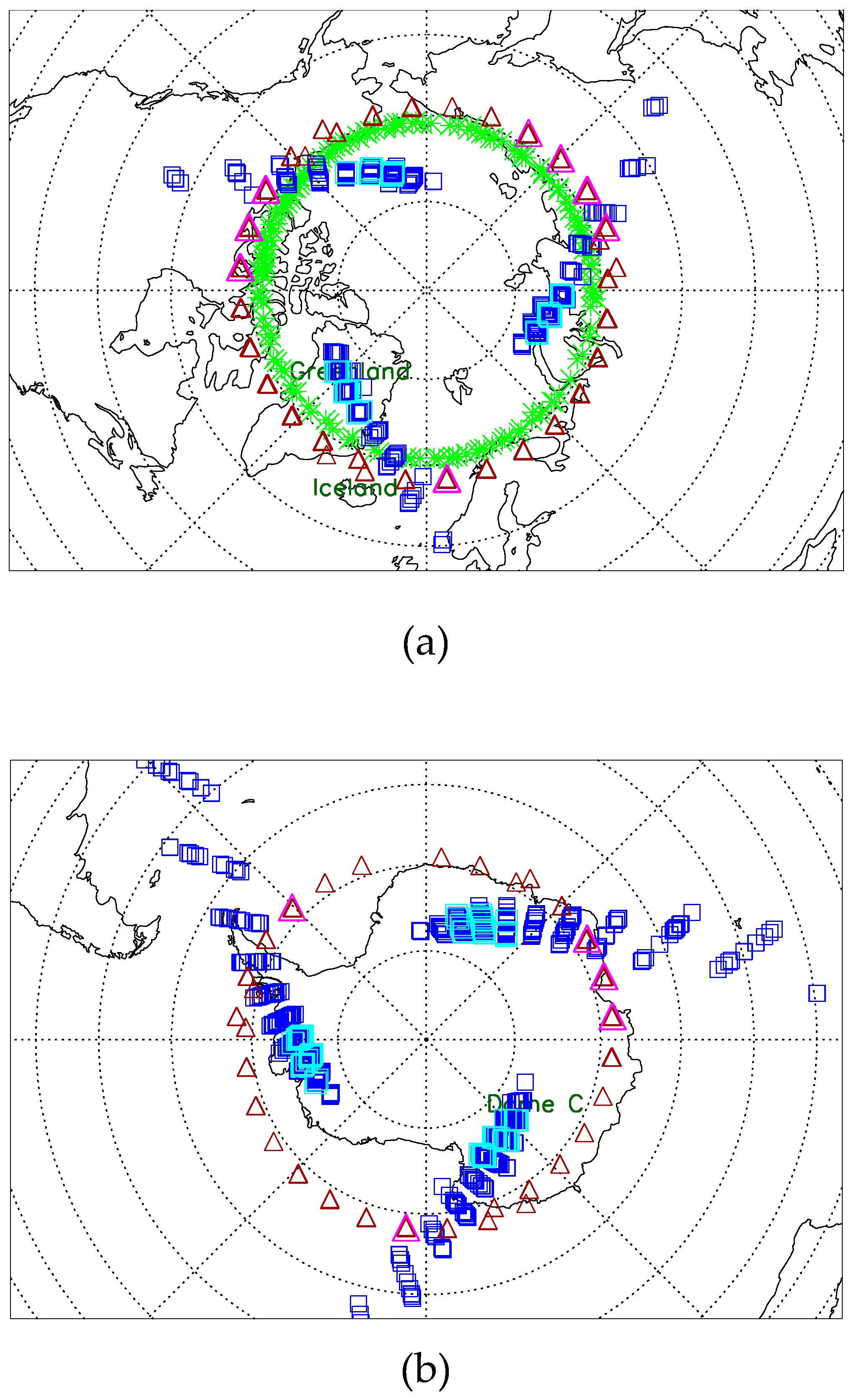
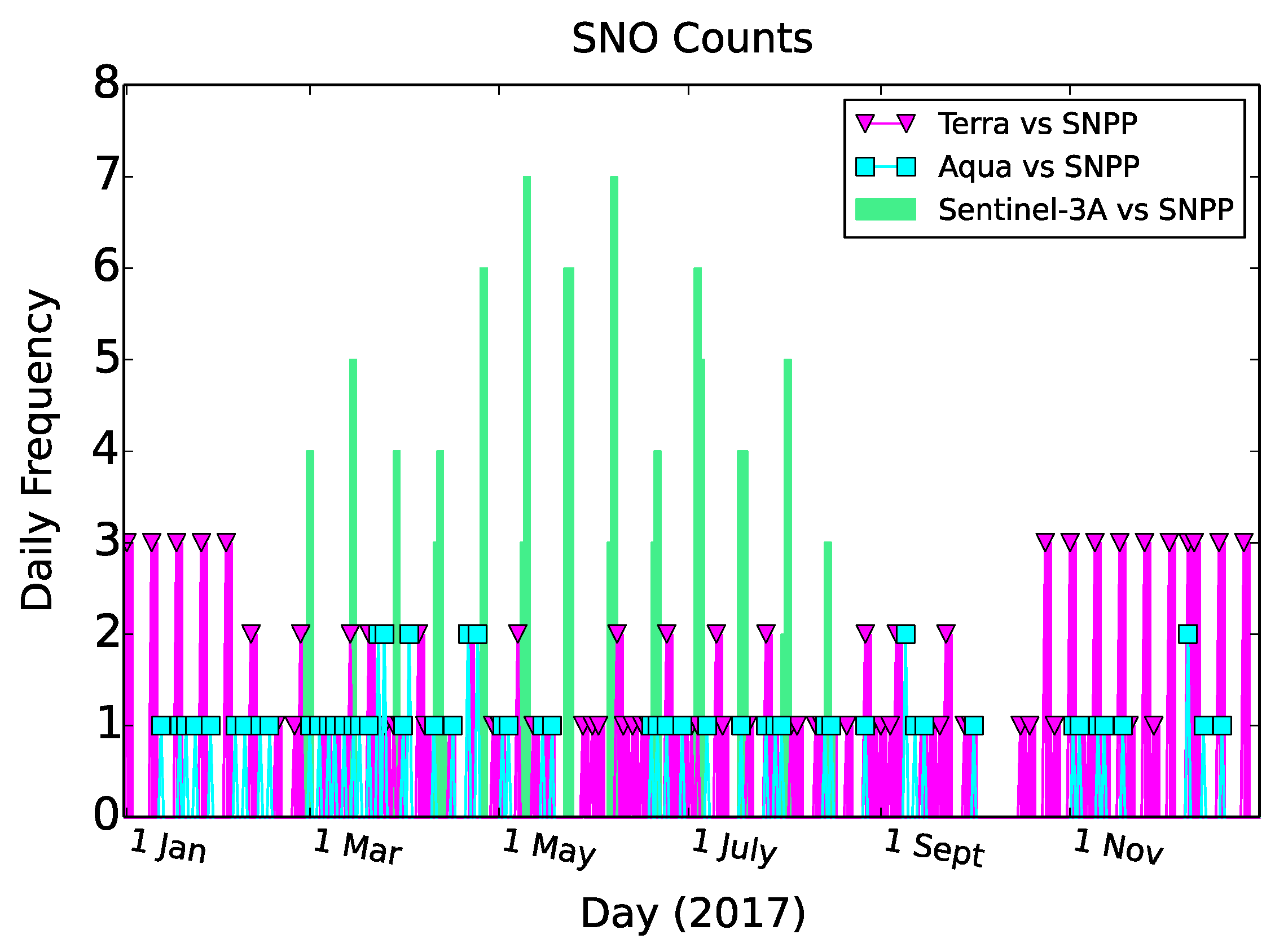
2.2.1. SNO Geolocation and Scenes

The occurrences of SNOs are determined by the flight trajectories of the satellites. Figure 2 displays the SNO locations for three pairs of satellites—Sentinel-3A versus SNPP for the year 2017 (red triangles), Terra (green stars), and Aqua (blue squares) versus SNPP (green stars) up to end of 2017—showing the northern polar region in Figure 2a and the southern polar region in Figure 2b. The 2017 SNO subsets are highlighted for Terra versus SNPP (magenta triangles) and Aqua versus SNPP (cyan squares); this is to illustrate that SNO locations do not repeat yearly. The SNOs of Sentinel-3A versus SNPP, with descending node for the former and ascending node for the latter, are concentrated within a tight circular band at around N71° latitude just inside the Artic Zone, with no occurrences in the southern region. On the other hand, the SNOs of Terra versus SNPP, also in opposing descending and ascending node, occur over both northern and southern regions, tracing out near the N68 and S68 circulars. The SNOs of Aqua versus SNPP, both ascending node, occur over both northern and southern polar regions in an interesting three-arm spiral pattern. This illustrates that different orbits and flight parameters map out different SNO locations, and therefore the reflectance property and the common atmospheric conditions of these SNO scenes are important factors. For example, Aqua versus SNPP commonly crosses over icy scenes of Antarctica, which have scene radiance commonly above 50 watt/m²/sr/μm, thus easily saturate SNPP VIIRS M6 and many MODIS bands of low dynamic range.

Figure 3 shows the daily frequency of precise SNO events for the year 2017. An interesting finding is the extended four-month periods of missing SNOs events for Sentinel-3A versus SNPP satellites (green bars) that run from October to February. Although not shown, the late 2016 and early 2018 periods are also without SNO occurrences for Sentinel-3A versus SNPP. A quick check confirms that Sentinel-3A OLCI observational coverage changes throughout the year and does not extend beyond 71° latitude during those four-month gaps, and therefore, despite any actual SNO events of the two satellites, there is no OLCI data available. Another interesting result of Sentinel-3A versus SNPP is that the SNOs cluster in distinctive days, 45 days of multiple SNO occurrences that further group into 13 clusters, thus showing that mismatching flight parameters, such as 16-day versus 27-day repeat cycle for this case, can generate interesting occurrences.

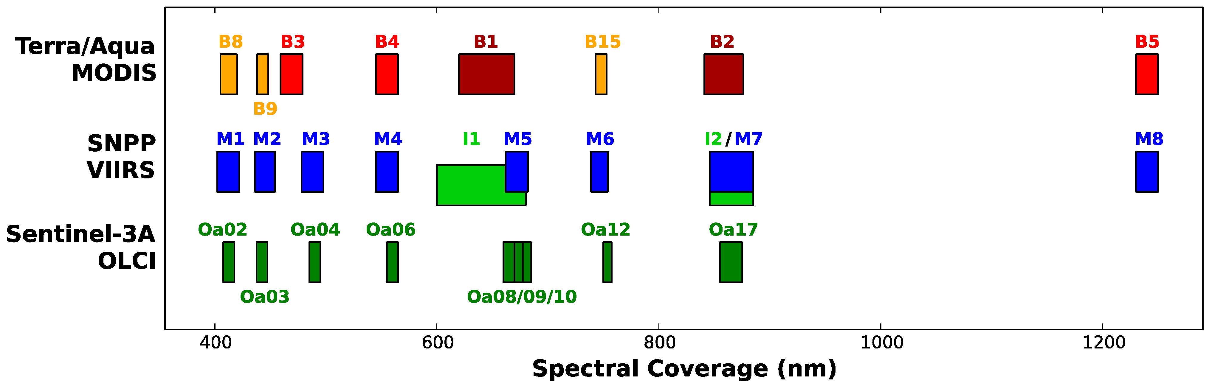
2.2.2. Spectral Match

The matching of two bands for radiometric comparison is customarily made according to their spectral proximity to ensure comparable radiometric responses over SNO scenes. In reality, most band pairs have RSR differences that induce yearly variability into the comparison time series. On the other hand, some band pairs not showing good spectral match, such as Aqua MODIS B3 versus SNPP VIIRS M3 with limited RSR overlap as shown in Figure 1, can still generate usable comparison time series [6,7]. A more extreme example is Aqua MODIS B7 (2130 nm) versus SNPP VIIRS M11 (2257 nm) [25] for which the two RSRs do not overlap but a marginally usable time series can still be generated. The impact of RSR mismatch and the full range of possibilities beyond the standard spectral-matching practice are not fully understood and should be pursued in future studies.

2.2.3. Dynamic Range

The limitation due the dynamic range is briefly presented here only for clarifications. The narrow dynamic range of a band can set a limitation impossible to overcome. For example, Aqua MODIS B15 (748 nm) versus SNPP VIIRS M6 (746 nm), with L_MAX of 3.5 and 41 watt/m²/sr/μm, respectively, hardly generates any successful outcomes as both bands saturate over the higher-latitude icy polar scenes where their SNOs commonly occur. However, future sensors with progressively wider dynamic range are less likely to encounter saturation. For instance, Sentinel-3A OLCI bands already have sufficient dynamic range and show no saturation issue for this study. But for band M6 of all VIIRS builds at only 41 watt/m²/sr/μm L_MAX, the success of SNOs involving VIIRS M6 is limited.

2.2.4. Spatial Resolution

The central goal of this study is to assess the capability of radiometric intercomparison and the achievable statistics in different regimes of spatial resolution. That is, how well can intersensor comparison assess radiometric performance of a sensor at different pixel sizes? As the regime reaches the 1-km resolution or so, the number of pixels in a small but realistic sized area selected for comparison becomes sufficient to allow standard statistical sampling. For example, at 1-km regime, a small area of 32 × 32 km-square contains 1024 pixels, which is sufficient for robust statistics under favorable scene conditions. The current result, such as shown in Chu et al. [7], suggests that the precision result of the time series at 1-km spatial regime is ~1%. Below the 1-km regime, the greater pixel density then give more samples per unit area as well as greater flexibility to enable more powerful sampling analysis—it may be possible to reach precision result much tighter than 1%. At coarser spatial resolution, for example at 5-km pixel size, to have 1000 pixels require an area size of 160 × 160 km-square, and that extent is too large to realize “nadir-only” condition. Therefore, the result using large coarser pixel size is likely to have large-area effects to render the result unreliable.

Most SNPP VIIRS and Aqua MODIS bands are moderate bands, at 750-m and 1-km spatial resolution respectively, and their intercomparison at the 1-km regime have demonstrated precision result at ~1% [7]. But Aqua MODIS and SNPP VIIRS also contain imagery bands with resolutions as fine as 250 m, and furthermore, the OLCI spatial resolution is ~300 m. The examination at regimes finer than 1-km can therefore assess the capability at higher imaging capability. The coming era will have more such higher spatial resolution imaging sensors, such as OLCI already in operation.

3. The Examination of Radiometric Intersensor Comparison

This study generalizes the methodology used in the Aqua MODIS versus SNPP VIIRS inter-RSB comparison by Chu et al. [7] to focus on three key criteria—area size, pixel homogeneity, and pixel sample size. The small area is a way to approximate the “nadir-only” condition, while homogeneity and sample size constraints are containment strategies to minimize a generally persistent scene-based variability of ~2% significantly impacting the comparison result. This persistent broad-scale variability—the “scaling phenomenon”—renders the use of larger area and sample size to improve statistics useless and is a key motivator of this study. The earlier assessment [7] suggests that the scaling phenomenon arises out of some mid- to large-scale scene conditions in the southern polar region, including Antarctica, where SNOs commonly occur. The application of the constraints to each SNO event successfully circumvented the variability to achieve a better precision at about 1%. This study clarifies how scene-based variability can impact intercomparison and why improvements can be made. The northern polar region is also shown to have the same 2% scene-based variability.

3.1. Procedure and Setup

Given an SNO event precisely determined within a single pixel of nadir crossing, a small area centered on the nadir crossing is used for pixel-based radiometric intercomparison. The radiance pixels of the two sensors within the small area are matched pair-by-pair via geolocation information. Each pair of collocated pixels is used to compute a pixel-based radiometric ratio of radiance. For this analysis, SNPP VIIRS radiance is taken to be the common radiometric reference against that of MODIS or OLCI. A fixed number of pixels of the best homogeneity quality, to be explained below, is selected for the computation of population statistics. The population average and the relative standard deviation (STD) of all qualified pixel-based ratios represent the ratio and the precision, or error bar, of the SNO event. The low radiance bias of MODIS and the impact of the solar zenith angle (SZA) are two issues briefly discussed here for clarification but are not used for analysis.

First, specific only to the inter-RSB comparison of MODIS versus SNPP VIIRS, a radiance cut of the 20% of the lowest radiance is imposed to remove biased cases occurring at low radiance, as was first done by Chu et al. [7] for Aqua MODIS-based result. The low radiance values from the two sensors are actually in good agreement on absolute terms, but nevertheless can result in large relative bias primarily as numerical artifact due to the low radiance value in the denominator. This low-radiance bias is also quickly confirmed to be true for Terra MODIS versus SNPP VIIRS. High radiance cases also possesses a few outliers, possibly associated with band response near saturation, thus the highest 10% of the radiance are removed as a safety measure. On the other hand, the OLCI-based comparison result does not exhibit bias at either low or high radiance. This points to MODIS possibly having some calibration issues, such as incorrect characterization of nonlinearity at low radiance, but is in any case a calibration issue not examined here.

The second issue concerns the impact of the SZA dependence, which imparts to radiance a distinctive seasonal pattern. However, the “nadir-only” restriction effectively cancels out the SZA effect in the radiometric comparison because the SZAs of the two sensors are effectively identical across the small area. Figure 4 shows the SZA correction ratio of Terra versus SNPP (magenta triangle), Aqua versus SNPP (cyan squares), and Sentinel-3A versus SNPP (green stars) for the year 2017. The error bars are mostly ~0.1% and smaller. Given the yearly cycle of the SZA, the demonstrated stability in the year 2017 is sufficient to show that the SZA correction factor will not impart to comparison time series any seasonal modulation or multiyear drift. The small random variability can be attributed to the time difference that is also random from one SNO event to next; furthermore, the accuracy of geolocation data can also be questioned at the level of 0.1%. Thus it is not necessary to include the SZA correction factor in the “nadir-only” framework.

3.2. Homogeneity

Homogeneity, or spatial uniformity, quantifies the variability of a pixel. It is most straightforwardly represented by the percentage STD calculated using the pixel itself and its eight neighbors—that is, the STD of the value of the nine pixels in the 3 × 3 square divided by the value of the center pixel. A few options exist for its application—at pixel-based radiance of each sensor, at pixel-based ratios computed from collocated radiance pixels, or both; it is tested for this study that for as long as homogeneity is applied, the result differs very modestly only in rare events. For simplicity, this analysis applies homogeneity to radiance data.

The primary importance of homogeneity lies with it being a proxy to statistical quality of pixel-based data to be used in tandem with a sample size constraint condition, to be described below. Homogeneity in this analysis is not simply an imposed threshold, but is used to generate a sorting of pixel quality to allow a selection procedure under a sample size constraint. Using only a simple homogeneity threshold will include all pixels satisfying the threshold, and different SNO events will have different sample size. On the other hand, using size-constrained selection forces all qualified SNO events to contain the same number of pixels, and this has the advantage of allowing more straightforward interpretations and comparison among events. A threshold of homogeneity, such as 4.5% as a reasonable level can always be imposed, but its importance to contain noise or variability becomes secondary when sample size constraint, itself a mechanism of containment, is used.

3.3. Area Size and Sample Size Constraint

The impact of area size, sample size constraint, the scaling phenomenon, and other associated issues of the comparison sampling analysis are examined here under expanded scope. The band pair of Aqua MODIS B5 (1240 nm) and SNPP VIIRS M8 (1238 nm) is used as the representative case study because their comparison result has shown to be the most stable [6,7]—this is primarily due to their well-matched spectral coverage and partly to the radiometric stability of the SWIR bands. For each SNO event, an examination of the impact of area and sample size is carried out at each spatial scale from the 20-km to 160-km scale. That is, 20 × 20 km-square area centered on nadir crossing is analyzed, then on to 32 × 32 km-square and so on until up to 160 × 160 km-square. At each scale or area size, statistics are computed for two separate cases. For the sample-unconstrained case, all pixels within the 4.5% homogeneity are used to compute the population statistics. In the sample-constrained case, only a fixed number of pixels of the best homogeneity quality, also necessarily below 4.5%, are used. The sample size of 500 samples and 1000 samples are used for the size-constrained cases.

The usable SNO events range from those of clearest scene conditions to those of variable conditions. A best-scenario SNO event is shown in Figure 5, that of 15 December 2016, for the sample-unconstrained case (red stars) and two sample-constrained cases, at 500 (green diamonds) and 1000 samples (blue squares). The top panel shows the average ratio of the qualified pixel-based ratios at each scale or area size, and the bottom panel shows the corresponding error bar, or the relative STD. The ratio result shows near-perfect broad-scale agreement among three cases that is remarkably stable at 0.991. The error bars are also very tight for all three cases, and are practically identical for the two sample-constrained cases at 0.2%. The overall result indicates a very clean scene condition that can generate very robust result at all scales shown up to 160 km. The occurrences of SNO events with this level of pristine clarity are only of several per year, but they remarkably reveal the capability of intercomparison to be fundamentally at the 0.2% level. The broad-scale agreement also reflects the sampling procedure to be meaningfully constructed and correct. All similarly clear-scene cases at other times have been checked to generate stable ratios and tight error bars across all scales as well. When clear SNO conditions exist, such as with low cloud or aerosol content, then using any small area size within the SNO scene will generate a robust and the correct result. It is here pointed out that Chu et al. [7,25] have examined one such high-precision event to confirm its clear-scene condition.

The primarily important SNO cases are those of marginal statistical quality with broad-scale error bar of few percent, approximately 2% to 4%, that can be improved to be below 2% to be added to the comparison time series. Thus the number of these marginal cases can determine the success or failure of a time series. Figure 6 illustrates two representative cases with ~2% broad-scale error bar. The labels are the same as those of Figure 5. The most outstanding feature to note is that, consistent over the entire range of scale or area size shown, the sample-constrained ratios are stable with tighter error bars, while the sample-unconstrained ratios are unstable at the level of 1.5% or worse. In particular, the ratio-versus-scale result of each sample-unconstrained case demonstrates worsening scatter toward larger scales—this decisively demonstrates the use of larger areas on its own does not improve comparison result and can in fact make it worse. Thus a strategy such as using larger areas or all available pixels, even when many noisy pixels have been removed via a homogeneity filter, is not a reliable procedure. On the other hand, the two sample-constrained cases—at 500 and 1000 samples—show stable ratio with broad-scale agreement. This finding shows that robust results are not achieved by having more samples but on the contrary by limiting them, specifically by using only the best-quality pixels. The error bar results of the constrained case are also tighter and continue to smoothly tighten further with increasing scale. The overall strong conclusion is that the application of sample size constraint, in conjunction with a homogeneity-ranked selection, stabilizes the ratio and tightens the error bar at each scale. Because of this stabilization, area size actually becomes statistically conforming—that is, by increasing the area size, more samples become available for selection and the error bar tightens as expected. The caveat is that fixing the number of best quality pixels is a necessary middle step to facilitate this conforming behavior.

The precision-versus-scale result (bottom panel) also illustrates distinctively different behavior between the sample-constrained and the sample-unconstrained cases. While the sample-unconstrained case exhibits unstable large scatter, the two sample-constrained cases instead show a smooth exponentially decreasing patterning of error-bar tightening that begins to agree at the 60-km scale and finally settling at ~1%. It is clear that the unconstrained case uses all pixels necessarily including all those of worse statistical quality, thus the inclusion of all pixels does not help to tightening the error bar but in fact worsens the result. An examination of the pixel quality (shown later) illuminates this point. The precision of the unconstrained cases also shows consistent clustering at around the 2% level throughout all scales, thus demonstrating instances of “scaling phenomenon” within individual SNO events. However the phenomenon is herein explicitly revealed to be only loosely scale-invariant, and that the error bar can vary with scale or area size to some degree. This is a common feature for a majority of SNO events.

The exponential shape of the error bar results also indicates some well-behaved property. For the 1000-sample case, the 32-km scale is where the area size is minimally large enough to have more than 1000 pixels, specifically at 1024, for the analysis to be applied. At this scale, both the constrained and the unconstrained results contain almost the same set of pixels, thus the two precisions necessarily are closely matched, as shown in both dates at ~2.3%. As the area size increases to include more pixels, the constrained case will have more available pixels from which to select those of best homogeneity quality to further tighten the error bar. The error bar stabilizes at larger scales when most pixels of best homogeneity quality have been found, and that finding more pixels of better homogeneity from larger area becomes both less probable and less leveraging. This finding suggests that the selection of area size and sample size should not be too tightly matched, and instead, given any sample size constraint, the area size should be made larger to allow more samples. For example, for comparison at the 1-km regime using 1000 samples, an area of 50 × 50 km-square with 2500 available pixels will be better than a 32 × 32 km-square area with only 1024 pixels. The precision result in Figure 6, showing tightening precision at larger area, proves this point.

The relative left-right shift in the error bar versus scale result demonstrates another aspect of the sample-size condition. As explained above, the 1000-sample case starts its first point at the 32-km scale; for the 500-sample case, 23-km is the starting point with 529 available pixels. In any given spatial resolution regime, sample-constraint size determines the minimal scale. Therefore future sensors with finer imaging capability will push the minimum area even lower, allowing for more refined studies and improved capability.

3.4. Examination of Pixel Quality

A closer examination into the homogeneity of pixels reveals some insights into their statistical quality. Figure 7 shows the homogeneity of 2000 pixels from the 50 × 50 km-square area in the 11 June 2016 event of Aqua MODIS B4 versus SNPP VIIRS M4, corresponding to Figure 6b, ranked from best to worst. The two vertical lines mark 500 and 1000 samples. The first 500 samples have homogeneity better than 3.5%, but the next set of 500 samples, from number 501 to 1000, ranges from 3.5% to 4.7%. It is clear that the first 500 ranked samples will generate smaller variability then the next 500 samples and so on. This is consistent with Figure 6 which shows the 500-sample case is actually more precise then the 1000-sample case. The ranking of homogeneity as in Figure 7 exposes that includes more pixels can bring in those pixels with greater variability and make statistics worse. While obvious as presented, this runs counter to the common expectation that a larger sample size would generate better, not worse, statistics. The continually rising pattern of homogeneity of ranked-pixels indicates different variability pixel-wise, thus a sampling analysis over SNO scenes does not conform to standard sampling where each data point conforms to the same variability. This is neither an obvious nor trivial property that is anticipated, but nevertheless is consistent with physical reality in hindsight. Therefore cleaning processes based on physical conditions, such as cloud removal, that focuses on a subset of pixels with specific physical attributes does nothing for this pixel-based variability and will not stabilize the statistics. The issue is not if the pixels have been cleansed of certain physical attributes but whether or not if too many pixels of higher variability have been sampled. The real physical conditions of Earth scene data can vary, and cannot be expressed by a single well-defined distribution. Inclusion of more samples to improve statistics is inherently erroneous and can end up broadening the distribution and worsen the error bar. Therefore the containment of the worsening statistics, such as limiting the sample size and using only the lowest variability pixels, is the necessary remedy.

Figure 7b demonstrates how average precision and average homogeneity increases with respect to the number of sample at three area sizes—36-km (red triangles), 50-km (blue squares), and 80-km scale (green diamonds). For each of three testing area sizes, average precision and average homogeneity are computed for each given number of the homogeneity-ranked pixels. For example, for the 36 × 36 km-square area case which has 1296 pixels, the best 100 pixels in terms of homogeneity are used for computation of statistics for the first point, and then 101 pixels of the best quality are used and so on. Expectedly, the average homogeneity and precision worsens with inclusion of more pixels. The three cases also show that statistics improve with larger area under sample constraint. The 11 June 2016 event is a marginal case, and its 36-km, 1000-sample precision result at 2.2% would have been excluded by a 2% precision requirement for the time series; but its 50-km, 500-sample result shows that a different set of criteria can improve pixel selection leading to significant improvement to 1.7% precision. A quick summary of the sample size constraint is that, large constraint size can worsen statistics but using larger area can improve them.

It is natural to want to find the optimal scale and sample size choice, but the answer does not require another thorough study, but rather simply on the caution of keeping the area size small enough to avoid potential hidden bias. While Figure 7 may shows that the 80-km scale (green diamonds) generates the best statistics, the overall finding including that of the unconstrained cases in Figure 6 also suggests the presence of some underlying bias over larger area. For the 1-km regime, the 50-km scale is an acceptable balance between having an area small enough to minimize the large area bias and one large enough for good, but not necessarily the best, statistics. The result also shows that sample size range of 400 to 600 to be reasonable.

The distributions of qualified pixel-based ratios per each SNO event are examined for the three different sample size conditions. Figure 8 shows the three distributions of the 29 May 2016 event at the 70-km scale to be normal-like, indicating that the samples as a set are well behaved in each case. The key point is that the 500-sample case has the tightest distribution, followed by the 1000-sample case and finally the unconstrained case. This is consistent with the result of Figure 6 showing 500-sample cases having lower error bars. Other scales are checked to have the same behavior. The broadening of the distribution from the 500-sample to the unconstrained case is the most direct demonstration of the lack of an underlying stable distribution, showing that the sampling in intercomparison involves physical data of different variability. By including more samples in the homogeneity-ranked scheme into the distribution, the result increasingly contains worse statistics to broaden the distribution.

It is worthy to clarify that the impact of homogeneity on error bar is neither direct nor absolute. Homogeneity as applied in this study has been shown to be a beneficial metric to help stabilize statistics, but pursuing into greater details is not necessary at the 1% precision level. It has been examined that slight variation at ~4.5% leads only to the slightest difference in a few SNO events. The sample size limitation and the selection procedure as described thus far are the main factors impacting the error bar result.

3.5. Application and Result

The long-term stability of the Aqua MODIS B5 and SNPP VIIRS M8 time series makes it an ideal case to illustrate the impact of various selection criteria. Figure 9 shows the three cases of 36-km with 1000 samples (red crosses), 36-km with 500 samples (green diamonds), and 50-km with 500 samples (blue squares). The solid line is the series mean set at 0.988 and the two dash lines mark the 2% boundaries above and below the mean. A precision threshold of 3% is applied to all three time series. The mean and the precision results are computed using the best 100 events in each time series for consistent comparison purpose.

It is seen that lowering constraint size has impact. Lowering the sample size constraint from 1000 (red crosses) to 500 (green diamonds) increases successful comparison outcomes from 101 to 162 and tightens the 100-event error bar average from 1.214% to 0.622%. The 50-km, 500-sample (blue squares) time series, contrasting against the 36-km, 500-sample case, increases the number of successful SNO events to 195 and tightens the error bar to 0.424%.

Nevertheless, all three time series generate statistically indistinguishable series means at 0.988, thus it may appears at first that different conditions do not matter. However, for other purposes such as generating a fuller time series with fewer data gaps, i.e., better regularity, a larger area size and a less stringent sample size constraint may be better. For example, the 50-km, 500-sample time series (blue squares) contains more outcomes in the year 2012 and 2013 than the other two cases. What is demonstrated is that the area size and the sample size constraint can be tuned to improve some characteristics of the time series such as regularity that can be helpful to evaluate the radiometric performance at certain period. Larger area sizes beyond 80-km scale and lower sample size down to 250 samples have been examined to result in no improvement, thus supporting the 50-km with 500-sample condition to be sufficiently optimal for Aqua MODIS B8 versus SNPP VIIRS M8.

Yet the same result reveals a limitation—the existence of data gaps, such as the 5-month Austral winter period years 2014, 2015, and 2016. While many SNO events do exist in these periods and the refined analysis here has improved the situation somewhat, the challenging conditions of low radiance and noisy scenes are difficult to overcome. This is definitely one area for continual improvement.

Figure 10 further illustrates Aqua MODIS B5 versus SNPP VIIRS M8 result for three scenarios at the 50-km scale—the constrained case with 500 samples of best homogeneity (blue square), the unconstrained case with all samples without homogeneity condition (red stars) and clear-scene subset of the 500-sample constrained case (green diamonds). The 500-sample constrained case is the same time series in Figure 9, also in blue squares, repeated here for comparison. The same 3% precision threshold is applied for the constrained and the constrained cases, and a 100-event choice is similarly made for consistent comparison. For the clear-scene time series, a 0.35% precision is further imposed on the constrained case to extract this subset. The first notable improvement is that the constrained case is significantly better at 195 outcomes and a 100-event precision of 0.424%, comparing with the unconstrained case at 166 outcomes and 1.059% precision. This is consistent with the result in Figure 9. Also, the clean scene time series with 38 best outcomes, those with error bars below 0.35%, trace out a long-term baseline at 0.989 that is very consistent with other cases. As already revealed by the event of 15 December 2016 shown in Figure 5, the clear-scene result should be closest to the “truth” of comparison result. The clean scene time series with ~0.3% average precision suggests that 0.989 reflects the true comparison baseline, and that other times series are highly consistent with this result—this finding can be very helpful in pinpointing the radiometric baseline and helping to ascertain other features. It is worthy to note again that “nadir-only” condition by using a small area, here at 50-km scale, is already itself a sufficiently constraining condition, and therefore even the unconstrained case can appear to have comparably acceptable result.

Intercomparison can expose a variety of different outcomes and features. Figure 11 shows the corresponding comparison result of Aqua MODIS B4 (555 nm) versus SNPP VIIRS M4 (551 nm) for the constrained (blue squares), unconstrained (red stars), and clear-scene (green triangles) scenarios. The same 3% precision threshold is applied for both the constrained and the unconstrained cases, and the best 100 events are used to compute the time series statistics. In comparison with Figure 10, it is clear that different band pairs have clear qualitative difference; for Aqua MODIS B4 and SNPP VIIRS M4, which center near the 550 nm spectral range, the stronger scene radiance leads to more successful events.

Although the examination into the physical cause of any deviation is not a purpose of this study, one Aqua MODIS B4 versus SNPP VIIRS M4 result reveals an important feature: in the four-year period from 2013 to 2017, an upward drift of ~2% can be seen, thus exposing some worsening on-orbit calibration error in either the IDPS-generated SNPP VIIRS M4 or the Aqua MODIS B4 of Collection 6 release. The clear-scene time series (green diamonds) is particularly lucid in tracing out both the multiyear drift and the yearly oscillation. The worsening calibration error comes from within the IDPS-generated radiance due to some nontrivial angular dependence in the reflectance property of the SD degradation [26,27,28,29] that has not been correctly captured by the standard on-orbit calibration methodology. This calibration error is neither trivial nor negligible, and can severely compromise product retrievals and climate studies. Thus establishing a meaningful and reliable time series, along with robust ratios and tight error bars, is a fundamentally important aspect of intercomparison methodology to enable correct assessments of the sensor data. Additionally, the seasonal modulation exhibited in the time series is typical of inter-RSB comparison of Aqua MODIS versus SNPP VIIRS [5,6,7]. Figure 4 has shown that the SZA correction is not a contributor to this modulation; the RSR mismatch is necessarily one of the contributing causes.

Also, in Figure 11, the unconstrained case shows significantly worse statistics than the sample-constrained case, again demonstrating the utility of these constraints despite using fewer samples.

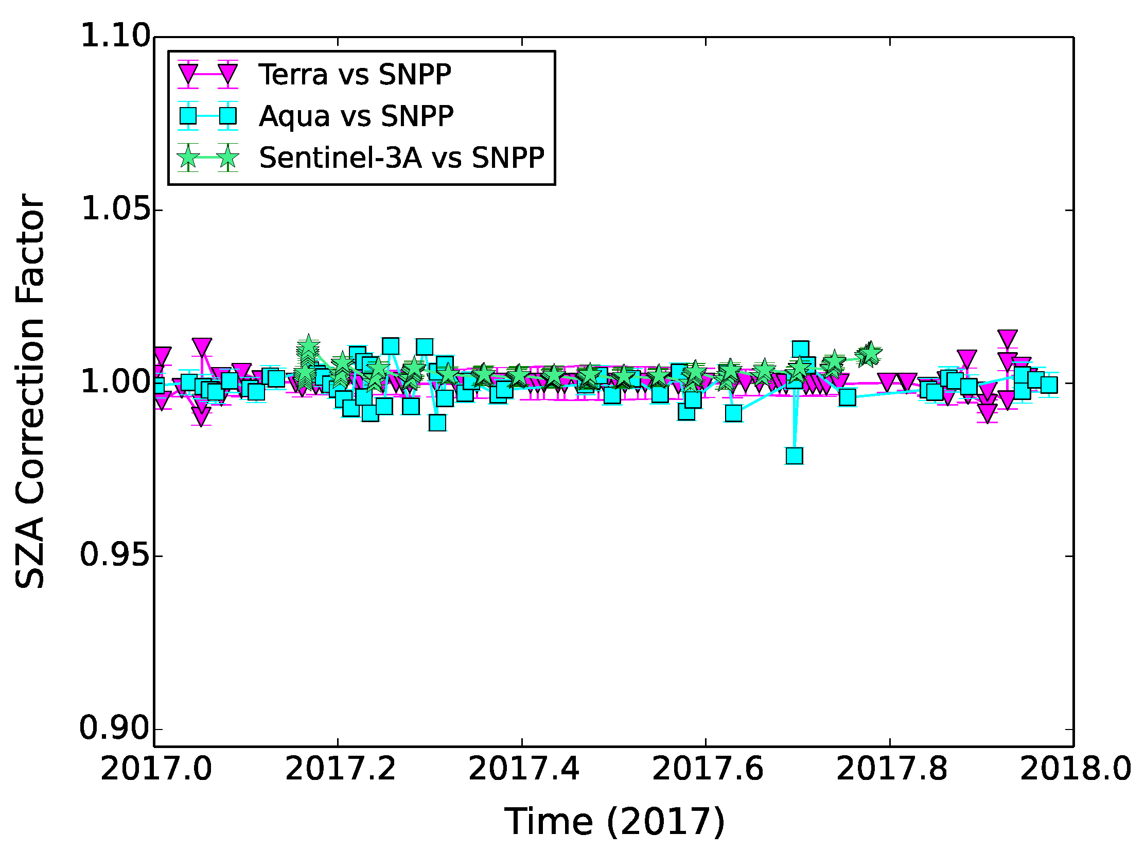
3.6. Impact of Precision Threshold on the Time Series

The current finding so far suggests a 0.2% stability of the overall ratio mean of time series under different scenarios, but additional examination of the dependence on the threshold over a larger threshold range yields some confirmation. Figure 12 shows the time series mean versus precision threshold of Aqua MODIS B5 versus SNPP VIIRS M8 for the four different constraint conditions over a 0.6% range. For each precision threshold, all SNO events under the threshold are included in the computation of the time series mean. As the precision threshold is relaxed, more SNO events with larger error bar are included, and the series mean changes accordingly.

The most important result is that the time series mean varies, primarily upward for this particular comparison case, over a 0.4% range with respect to precision threshold. The overall pattern is consistent with those events of tightest precision being more likely representative of the true radiometric comparison result, and those events of worse precision contain more radiometric bias. Therefore keeping a tight precision threshold is recommended to reduce any nontrivial variability or bias in the time series mean. The 2% precision threshold appears to be a reasonable choice with variability of the mean on the level of 0.2% variability in the mean for this context of the constrained procedure; while a more generous choice to achieve fuller time series must be cautious about making the time series mean less reliable.

The long-term stability of the Aqua MODIS B5 versus SNPP VIIRS M8 time series is what makes clearer the existence of any deviation or variability. In contrast, cases such as Aqua MODIS B4 versus SNPP VIIRS M4 with significant drift, as shown in Figure 11, are more difficult for interpreting the dependence on the precision threshold since the 2% drift complicates the result. For these cases, the mitigating the on-orbit calibration error should take top priority over any intercomparison issue. As emphasized already, intercomparison analysis is most valuable when it reveals some deviating that requires correction.

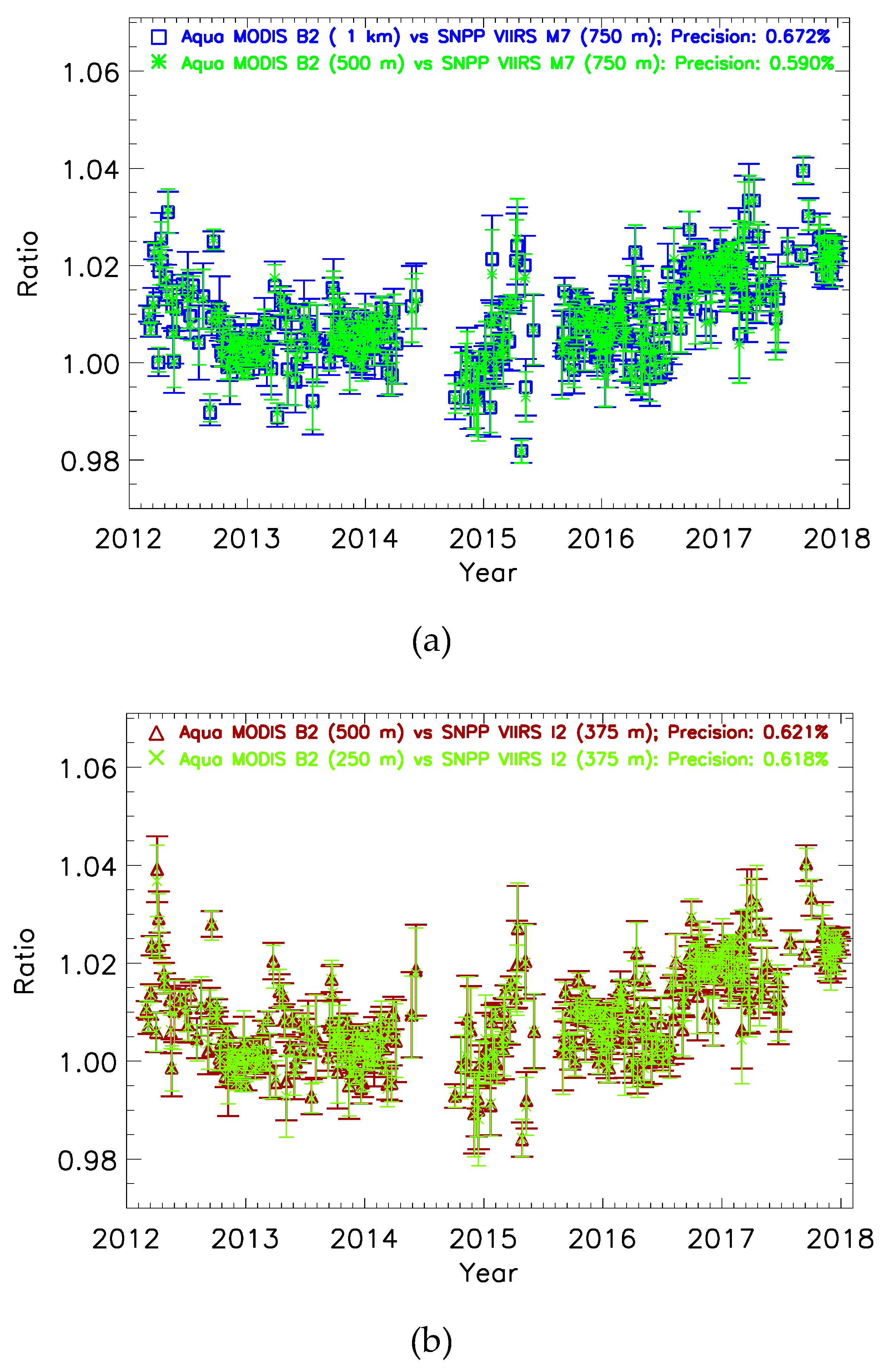
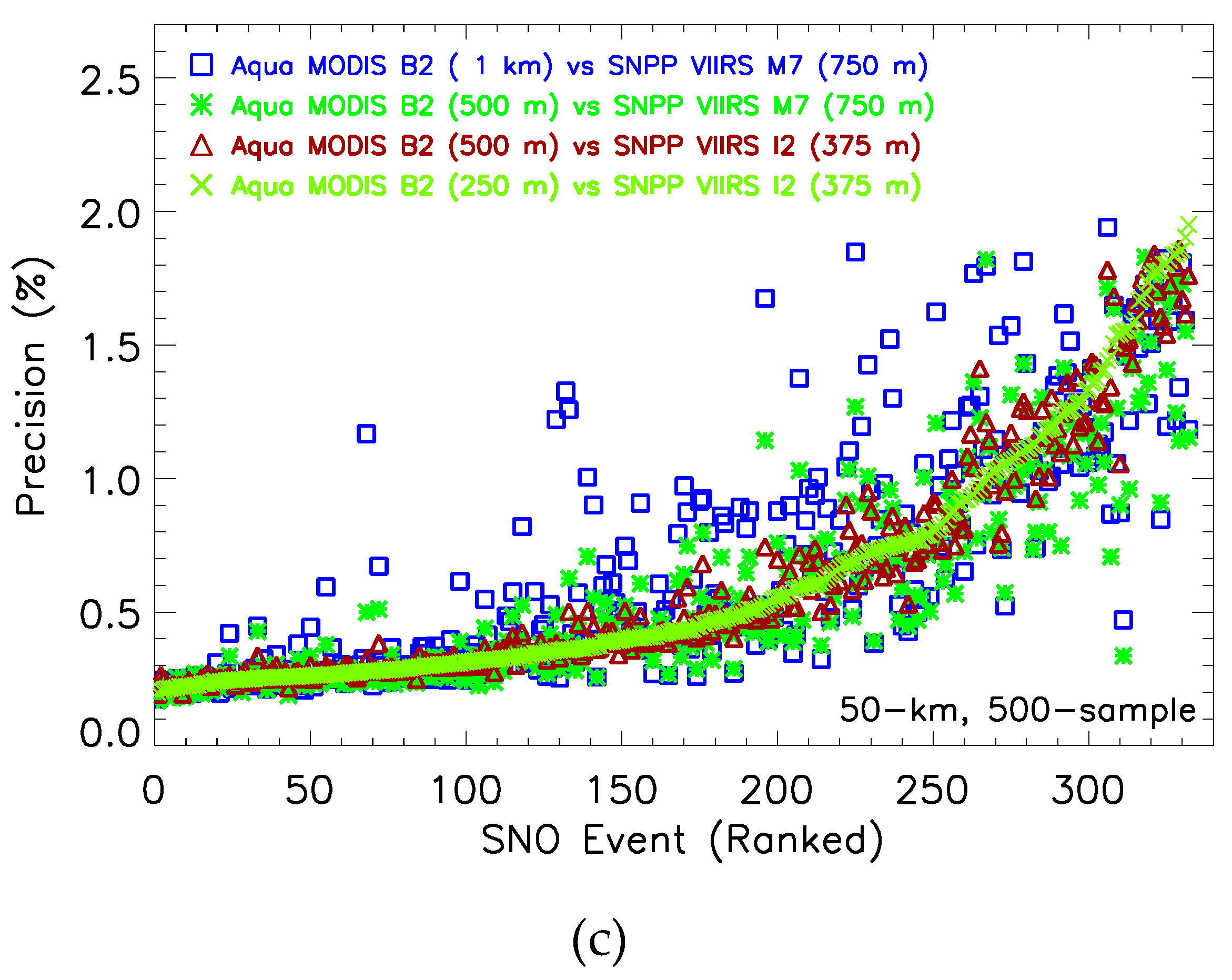
3.7. Scaling Phenomenon in MODIS versus SNPP VIIRS

The “scaling phenomenon” [7] is a broad-scaled and persistent variability pervading into the SNO results as illustrated in Figure 6 in selected events. Figure 13 illustrates the phenomenon for the Aqua MODIS B8 versus SNPP VIIRS M1 time series as a whole and includes the new result under the constrained analysis. Each point represents the error bar versus sample size outcome of an SNO event in the time series. Time series results of three different area sizes are shown: 36-km scale (red triangles), 50-km (blue squares), and 80-km (green diamonds). The result demonstrates how the scene-based scaling phenomenon blocks the use of the larger area size to improve statistics and how the constrained procedure overcomes this limitation.

The top left panel of Figure 13 displays the time-series result of error bar versus sample size (for all events) without size constraint. The maximum sample size for the 36-km scale is 1296, or close to 0.2 per 6400 on the plot, and similarly for the 50-km scale at 2500, at near 0.39, and 80-km at 6400, at 1.0. It can be seen that the pattern of scatter of error bar values, apart from different sample size ranges, appear similar for all three scales. The top right panel of Figure 13, the scaled version, explicitly demonstrates the scaling phenomenon by linearly scaling the sample size of 36-km and the 50-km result to match 6400, i.e., stretching the result in the horizontal direction rightward until 6400. The scaled result shows that scatter pattern of three cases are effectively indistinguishable. The clear implication is that enlarging the area size to increase the number of pixels ends up generating same statistics and does not improve the quality of the time series. In contrast, the time series results in Figure 9 under homogeneity-ranked sample constraint, demonstrate clear improvement with lager areas. More detailed examination into each SNO event reveals that the scaling phenomenon is only an approximate effect of some common scene-based effect. As shown in Figure 6, the error bar result in the sample-unconstrained case (red stars) in each single NO event can slightly change with increasing scale.

The sample size constraint, originally applied to stabilize the error bar [7], necessarily impacts any scene-based effects including the “scaling phenomenon”. The bottom two panels of Figure 13 demonstrate the impact of the constraints, for sample size of 500, on error bar versus sample size result. The label of “Sample Size” on the horizontal axis refers to the original available number of pixels for each event before the constraint is applied—thus it corresponds to the sample size for the corresponding unconstrained case. However all actual outcomes have the same final sample size of 500. In the bottom-right panel, the error bar scatter pattern of the 80-km result (green diamonds) is seen to become tighter than those of the 36-km and the 50-km scales, thus showing that scaling phenomenon is no longer true in the constrained analysis. In the same plot, the range of the error bar shows more obvious and faster tightening with increasing size for all three cases, reaching below 2% at higher sample size, showing that the constrained procedure is effective.

For completion and illustration, the corresponding ratio versus sample size of the Aqua MODIS B8 versus SNPP VIIRS M1 time series is shown in Figure 14. The 4 to 6% range of spread makes it less obvious to discern any 0.1 to 0.5% effect, but many resulting points can be seen to have shifted from the unconstrained case (top panels) toward the center of the range in the constrained case (bottom panels). The 4 to 6% spread of Aqua MODIS B8 versus SNPP VIIRS M1 ratio result is among the worst comparison results, whereas cases such as Aqua MODIS B5 versus SNPP VIIRS M8, as in Figure 8, spreads over a smaller 2% range. In general, ratio result is not an effective discriminator of statistical quality among SNO events given its large spread, and the final selection of the times series events should not rely on using ratio. On the other hand, error bar result, as shown by the bottom panels of Figure 13 as well as in earlier figures, has demonstrated to be stronger discriminator of statistical quality of SNO events that can be utilized as a selection filter.

The scaling phenomenon exists in effectively identical fashion for all inter-RSB comparisons of Aqua MODIS versus SNPP VIIRS. Figure 15 shows the scaling phenomenon for six inter-RSB comparisons of Aqua MODIS versus SNPP VIIRS. Be it thin clouds, aerosol, or any combination of scene conditions, it appears that some atmospheric conditions in the polar scenes impact all RSBs in nearly identical way. A general implication is that any inter-RSB comparison between any two polar-orbiting multispectral sensors that generate SNO scenes over the polar regions necessarily needs to take this scene-based effect into account.

Figure 16 demonstrates that the scaling phenomenon also exists for Terra MODIS versus SNPP VIIRS, exemplified by Terra MODIS B8 versus SNPP VIIRS M1. As Terra versus SNPP SNO events trace out completely different locations (see Figure 2), this result generalizes this scene-based variability over both northern and southern polar scenes.

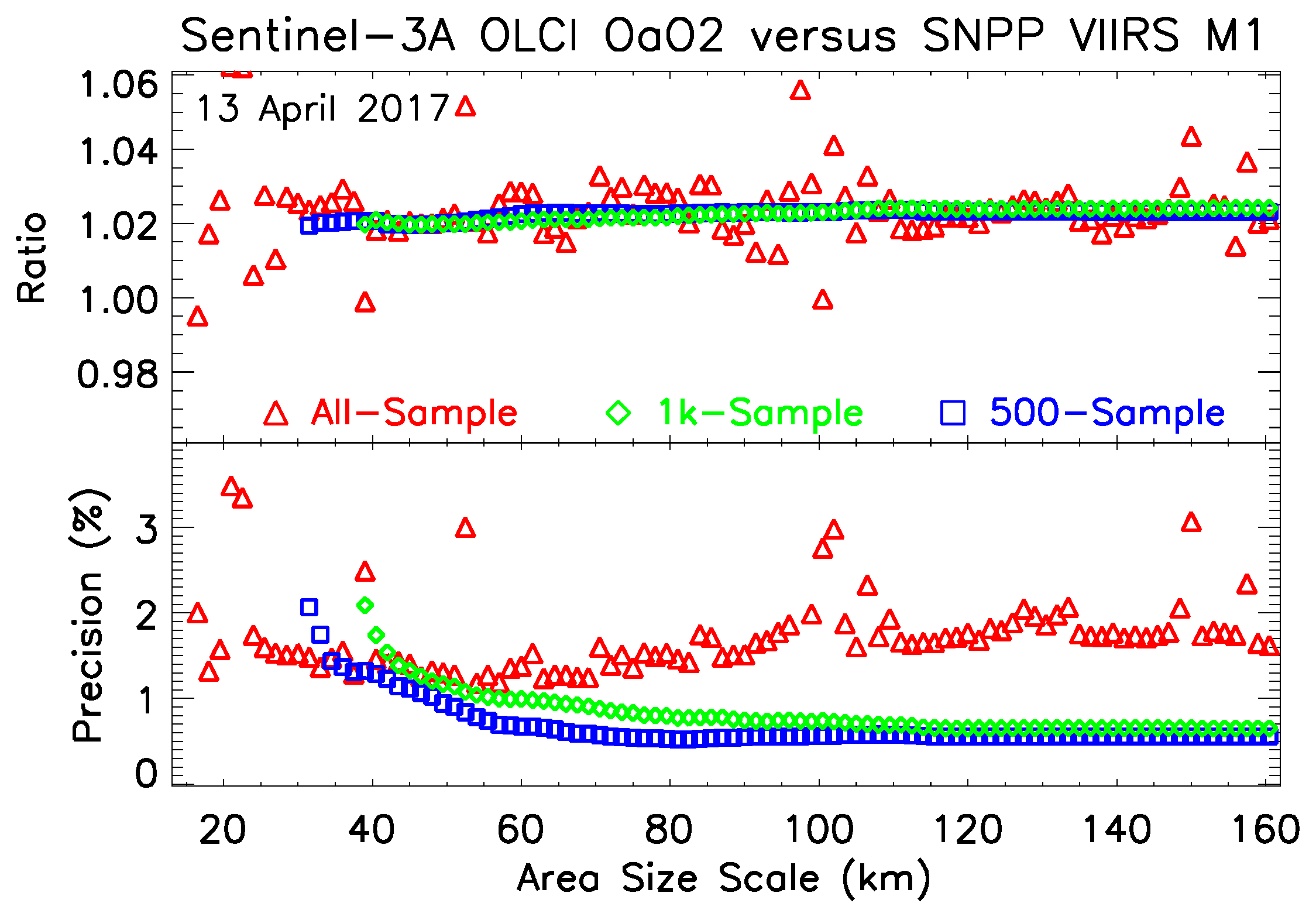
3.8. Scale-Dependence in Sentinel-3A OLCI versus SNPP VIIRS

Sentinel-3A OLCI is yet without enough SNO data to demonstrate the scaling phenomenon in full a time series result, but the scale-dependence can be examined within individual SNO events as done in Figure 6. Figure 17 shows the dependence of ratio (top) and error bar (bottom) on area scale for Sentinel-3A OLCI Oa02 (412.5 nm) versus SNPP VIIRS M1 (410 nm), for a 13 April 2017 event for the three cases of unconstrained sample size (red triangles), constrained size at 1000 samples (blue squares), and constrained size at 500 samples (green diamonds).

All features of the OLCI-based result effectively repeat identically. This result reinforces the recommendation to confine the SNO analysis to a “nadir-only” condition using small area and that scaling phenomenon is a general effect impacting any inter-RSB comparison of two polar-orbiting instruments.

3.9. Discussion and Summary

The key finding is that a homogeneity-ranked, sample size constrained sampling procedure under a small-area restriction stabilizes the ratio against some broad-scale variability to generate result that is reliable and robust. A smaller area size such as under the 50-km scale contains enough pixels for the refined sampling procedure but simultaneously avoids the pitfall of large-area or large-angle bias. As the ratio result has been stabilized, the application of various criteria, such as scale or homogeneity threshold, is further shown to have impact on the comparison time series.

Since Aqua MODIS B5 versus SNPP VIIRS M8 is one the most stable inter-RSB comparisons due to good spectral match and long-term radiometric stability, the average precision of the time series at ~1.0% very well represents the general statistical capability of inter-RSB comparison at the 1-km regime. While the clear-scene result such as in Figure 5 is remarkably stable and precise at 0.2% or so, its number is not sufficient for full evaluation. In general, radiometric comparison time series are best used as a tool of discovery of deviating features such as the multiyear drift.

Also important is the generality of the scene-based variability over both polar regions as shown in the inter-RSB comparison results of MODIS and OLCI versus SNPP VIIRS. Therefore, any inter-RSB comparisons of polar-orbiting multispectral sensors necessarily need to treat this polar scene variability with some care.

4. Capability at Different Regimes of Spatial Resolution

An assessment of the intercomparison at finer regimes of spatial resolution provides an understanding of what capability can be achieved in the coming era. For this purpose, the inter-RSB comparisons using SNPP VIIRS M7 (862 nm; 750 m) and I2 (862 nm; 375 m) against Aqua MODIS B2 (859 nm; 250 m), and Sentinel-3A OLCI Oa17 (865 nm; 300 m) are used to test four regimes of spatial resolution. Because the RSRs of SNPP VIIRS M7 and I2 are effectively identical, intercomparisons against them directly shows the impact of different spatial resolutions. In addition, Aqua MODIS B2, at 250-m native spatial resolution, also comes with aggregated data at 500-m and 1-km resolutions (Table 2) and provides direct testing of different spatial resolutions

The four regimes of spatial resolutions to be tested are described as follows. First, SNPP VIIRS M7, at 750-m, can be matched with the aggregate 1-km and 500-m data of Aqua MODIS B2, generating comparisons at the 1-km and 750-m regimes. Second, SNPP VIIRS I2, at 375-m, can be matched with the aggregate 500-m and the native 250-m data of Aqua MODIS B2, generating comparisons at the 500-m and 375-m regimes. For each pairing, the regime of intercomparison is defined by the lower spatial resolution. For Sentinel-3A OLCI at 300 m, the match with SNPP VIIRS M7 will be at the 750-m regime, and the match with SNPP VIIRS I2 will be at the 375-m regime.

Figure 18a shows the time series of Aqua MODIS B2 versus SNPP VIIRS M7 at the 1-km (blue squares) and the 750-m (green stars) regime for the first six years of SNPP VIIRS mission; Figure 18b shows the time series of Aqua MODIS B2 versus SNPP VIIRS I2 at the 500-m (red triangles) regime and the 375-m (cyan crosses). The precision threshold for each SNO event is 3%. The two times series in each plot have been carefully selected and matched to allow unambiguous event-to-event comparison. The time series cleansed and used here for illustration are otherwise slightly different from result strictly from the prescribed constrained procedure. The key and unexpected finding is that the three finer regimes appear only fractionally better than the 1-km regime—this hints at a lower limit of the statistical capability of the inter-RSB comparison methodology, or perhaps an additional physical effect at the level of 750-m scale. This can be an issue worthy of future pursuit.

For a more explicit demonstration, Figure 18c shows the precision result ranked from the tightest to the worst, but using the SNO events of the 375-m regime time series shown in Figure 18b as the reference of ranked events—the purpose is to reveal the statistical quality of individual events at different regimes. The SNO events of the 375-m regime (cyan crosses) are first sorted according to their precision from best to worst, and then results of other three regimes following the same SNO event sequence are plotted accordingly. That is, the 1-km, 750-m and the 500-m regime result are not separately sorted, but follow the same sorting event-by-event as that of the sorted 375-m regime result for comparison.

First, all of the most precise SNO events converge toward the beginning of the plot at about 0.15% to 0.2% precision, and this is because of the excellent homogeneity of clear-scene events. This indicates the comparison analysis has the inherent capability to reach 0.15% level. Second, the ranked result shows different intervals of slightly different pattern—a smooth pattern up to event 200 under 0.6% precision, followed by a stronger increasing pattern with more noise from event 200 to 350 and up to 2% precision, and finally the sharply rising and noisy pattern after event 350 and 2% precision. This even-by-event showing of the precision quality reveals the how precision threshold may be decided for a time series. For these cases, a 1.0% precision threshold seems a good balanced choice between having tight error bars and number of events. Third and most importantly as a focus of this examination, the result of the 750-m (green stars) and 500-m (red triangles) regimes can be seen to evenly straddle around the 375-m (cyan crosses) regime result, showing consistent agreement among the three finer regimes. On the other hand, the 1-km precision result (blue squares) is on the average higher than the result of three other regimes, as already revealed in Figure 18a,b. The capability of the radiometric intercomparison methodology, at least in the context of the constrained procedure, may have reached optimal result at the 750-m regime.

The time series also reveal some deviating features indicative of some basic on-orbit calibration issues. Although it may deceptively appear that the time series exhibits long-term drift, the result is more consistent with a series of radiometric jumps, suggesting numerous calibration adjustments for Aqua MODIS B2 or SNPP VIIRS M7/I2.

The Aqua MODIS versus SNPP VIIRS results shown in Figure 18 are statistically dominated by events over the southern polar scenes, easily noticeable for the clustering of events during the Austral summer period from October to March. To demonstrate events over the northern region, Figure 19 shows the two inter-RSB comparisons of Sentinel-3A OLCI Oa17 (865 nm) versus SNPP VIIRS M7 at the 750-m regime (green diamonds), and versus I2 (862 nm) at the 350-m regime (orange crosses). The two OLCI-based times series are also time-matched to ensure event-by-event correspondence. The subset of the Aqua MODIS B2 versus SNPP VIIRS I2 comparison in Figure 18b occurring in the northern polar region is also shown (cyan diagonal crosses) in Figure 19 for comparison. The three precision results illustrate similar statistical performance at the 750-m and the 375-m regimes, at ~1%, with no clear advantage of the 375-m regime over the 750-m regime. The two OLCI-based times series also demonstrate an overall event-by-event consistency of precision between the two regimes, as also shown by the Aqua MODIS-based result in Figure 18. The combined findings of Aqua MODIS-based and OLCI-based results show that precision result for comparison under 1-km regimes in either polar regions is consistently at ~1% and slightly less.

5. Multi-instrument Cross-Comparison

Intercomparison becomes even more useful when three or more sensors of comparable performance capability can be cross-checked. The next few figures exemplify the cross-comparisons of Aqua MODIS, Terra MODIS, and Sentinel-3A OLCI against SNPP VIIRS for the year 2017. The MODIS versus SNPP VIIRS comparison is carried out at the 1-km regime while that of OLCI versus SNPP VIIRS is at the 750-m regime. The time series are plotted over a 20% range centering on the time series means of the OLCI versus SNPP VIIRS, with two dashed lines marking the 2% level above and below the series mean. The applied precision threshold is 3%. The final figure shows the comparison result of three OLCI bands overlapping with SNPP VIIRS M5, explicitly demonstrating the impact of various level of mismatching RSRs. The impact of the spectral mismatch on time series remains one fundamental issue not yet adequately explored by the intersensor community.

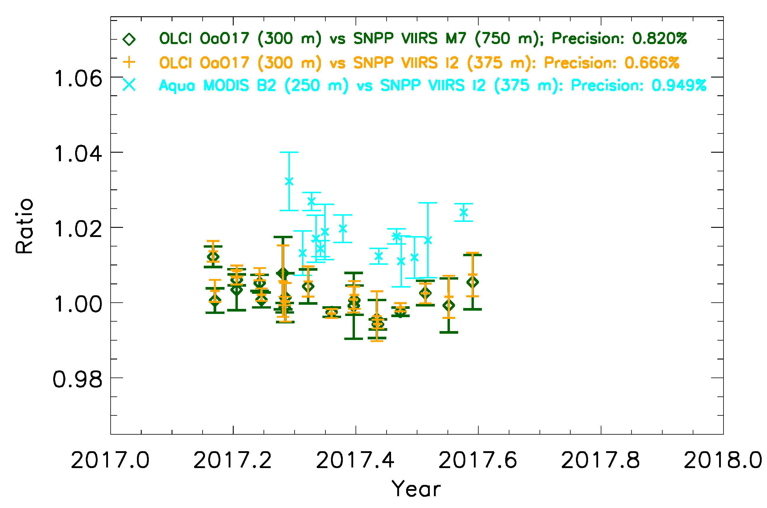
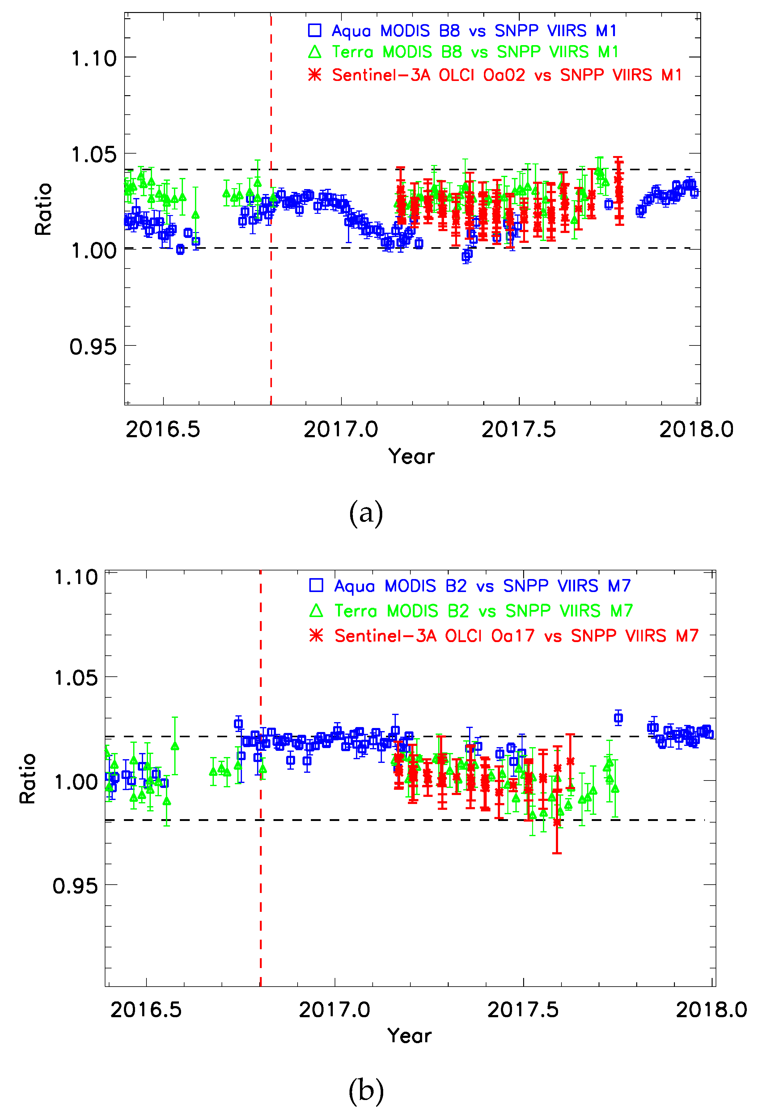
5.1. Aqua MODIS, Sentinel-3A OLCI and SNPP VIIRS Comparisons

Figure 20a shows the three comparison time series using Aqua MODIS B8 (blue squares), Terra MODIS B8 (green triangles), and Sentinel-3A OLCI Oa02 (red crosses) against SNPP VIIRS M1. It is seen that OLCI Oa02-based result is stable within 1% without strong seasonal modulation and short-term drift. On the other hand, the Aqua MODIS B8-based result reveals a 3% peak-to-trough seasonal variation beyond the 1% error bar, while the Terra MODIS B8-based result is of 2% seasonal variability along with a 2% difference with that of Aqua MODIS B8. Certainly, spectral mismatch between MODIS B8 and VIIRS M1 can induce seasonal pattern in both time series, but it remains possible that some physical or optical effect is impacting both Terra and Aqua MODIS B8. In addition, the discrepancy between the two MODIS-based results points to some inconsistency in the on-orbit calibration of MODIS B8.

Chu et al. [7] have previously concluded that IDPS-generated radiance for SNPP VIIRS M1 contains a long-term drift of approximately 0.4% over the four-year period from February 2012 to February 2016. For this recent 16-month period, the drift in IDPS-generated SNPP VIIRS M1 radiance is estimated to only ~0.15%, which is too small to be seen in these time series. The result suggests that OLCI Oa02 is not likely to have any significant short-term drift over the 16-month period.

Figure 20b shows the three comparison time series against SNPP VIIRS M7 using Aqua MODIS B2 (blue squares), Terra MODIS B2 (green triangles), and Sentinel-3A OLCI Oa17 (red stars). This set of bands is a clean case study due to well-matched RSRs, thus providing a good example of multisensor cross-check that can identify radiometric deviations. The precision is 1.15% for Aqua MODIS B2 result, 1.55% for Terra MODIS result, and 1.74% for OLCI Oa17 result. It is seen that both Terra MODIS and OLCI agree well with SNPP VIIRS M7, with time series consistent at ~1.0, as expected. However, Aqua MODIS B2 shows a clear upward shift of ~2% against SNPP VIIRS M7 starting sometime between May and October 2017. This discontinuity had been documented in a preliminary study [30] but the times series is extended here to make clearer the upward discontinuity. Based on the overall result, it is concluded that Aqua MODIS B2 went through the 2% radiometric jump just before October 2016.

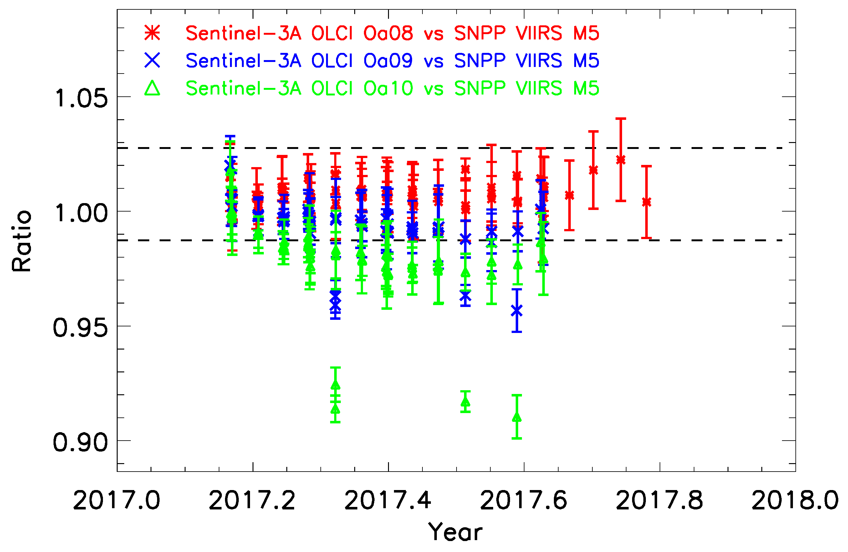
5.2. Impact of RSR Mismatch: Sentinel-3A Oa08-Oa10 versus SNPP VIIRS M5

The impact of the spectral coverage mismatch between two bands is nontrivial to quantify for intercomparison and is so far not well addressed or even well understood. The two primary effects of the mismatch are the offset from 1.0 in radiometric ratio and the emergence of yearly modulation. Here, only a demonstration of the effect is intended through an illustrative example using SNPP VIIRS M5 as a fixed reference and a set of three adjacent bands in Sentinel-3A OLCI. As shown in Table 2, the three OLCI RSBs, Oa08 (660–670 nm), Oa09 (670–677.5 nm), and Oa010 (677.5–685 nm), cover the 660 to 685 nm spectral region in sequence, with each having some spectral overlap with SNPP VIIRS M5 (662–682 nm).

The three inter-RSB comparison time series are shown in Figure 21 for the year 2017, for Oa08 (red stars), Oa09 (blue diagonal crosses), and Oa10 (green triangles). The three time series have nearly identical precision at 1.76%, yet differences among them are clearly shown. First, different radiometric offsets away from 1.0 expectedly show the dependence on the level of RSR mismatch. Second, while Oa08-based time series seems stable, both Oa09- and Oa10-based time series exhibit greater seasonal modulation, in particular, the Oa10-based result has the largest deviation at ~3%, not accounting for the three outliers below 0.95. This is the definitive demonstration of the different responses to the same set of SNO scenes arising only because the effect of mismatching RSRs. As Oa10 result indicates of it having the largest impact of the spectral mismatch with SNPP VIIRS M5, it shows both the largest downward offset and the most variable seasonal modulation in a consistent manner that is expected. However, what is not clear is how certain mismatch has less impact on the time series than others, such as OLCI Oa08-based result having weaker modulation. Nevertheless, the connection between the offset and the seasonal modulation is direct, that both being the manifestation of the spectral mismatch. Specifically, this connection may be useful for quantifying the impact of spectral mismatch.

The three outliers are briefly discussed here as an instance of multimodality. The outliers of each time series correspond to the same SNO events of the other two but at different ratios. These cases can arise from some scenes of less stable condition, such as cloudy or ocean scenes, which on occasions can still be stable enough to pass selection criteria. These cases are technically the result of a different mode, arising from the nontrivial effect of mismatching RSRs responding to different scene conditions. As has been pointed out previously, the presence of outliers or additional modes is one scenario where a targeted removal of certain scene condition, such as cloud, can be applied.

6. General Discussions

Intercomparison of radiometric data, as in any statistical sampling, is not entirely useful without a reliable estimate of error bars. The procedure described herein establishes the reliability of the error bars, or precision, of the comparison events, further making error bar a usable discriminator for selecting best-quality SNO events. The overall result shows that an overall 1% precision is reachable at the 1-km resolution. The constructed multiyear time series, “as is” without adjustment, are capable of capturing various features illustrative of some underlying radiometric or calibration issues as listed below.

1. Long-term drift reveals a systematically worsening error in the on-orbit calibration of the sensor data, as exemplified by Aqua MODIS B4 versus SNPP VIIRS B4 in Figure 11.

2. Sudden radiometric shift reveals a likely one-time calibration adjustment or instrument change as exemplified by the jumps in Aqua MODIS B2 versus SNPP VIIRS M7 before Oct 2016 shown in Figure 20b.

3. Noise and variability reveals scene-based effects as exemplified by almost all inter-RSB comparisons of Aqua MODIS and SNPP VIIRS in Figure 11, Figure 12, Figure 13, Figure 14, Figure 15, Figure 16 and Figure 17.

4. Seasonal modulation reveals impact of RSR or other physical effects as exemplified by Aqua MODIS B8 versus SNPP VIIRS M1 in Figure 20a and most demonstratively the three OLCI-based time series in Figure 21. Multimodality can also manifest from RSR mismatch. Definitively the seasonal modulation is not an issue related to the SZA.

5. Non-seasonal and sporadic shifts reveal possible calibration instability as exemplified by Aqua MODIS B2 versus SNPP VIIRS M7/I2 in Figure 18a,b.

6. Discrepancy between the different intercomparisons, in addition to possibilities listed above, can reveal additional biases and calibration inconsistencies, as exemplified in the cross-comparisons of Figure 19, Figure 20 and Figure 21.

So far, this study focuses on the on-orbit performance of the multispectral sensor data in the context of standard operational on-orbit RSB calibration. But the complete evaluation must include sensor data over all extent beyond nadir. It is therefore important to continue to distinguish between the issues of on-orbit RSB characterization from those of other additional calibration adjustments. One such important associated issue is the time-dependent RVS effect of the scan mirror that is known for MODIS [20], although not known in VIIRS and not yet addressed in OLCI. The full calibration of the sensor data for MODIS Collection 6 [19,20] involves additional correction necessary to mitigate this angle-dependent effect throughout the entire spatial extent that cannot be analyzed by the standard on-orbit calibration analysis. While the “nadir-only” framework of intercomparison can expose issues of standard operational on-orbit calibration, it is not designed to address any large-extent issues such as RVS. Nevertheless, this study puts forth a spatial scale-dependent analysis possibly extendable to examine off-nadir issues. The result of this study supports a strategy to first isolate and examine on-orbit calibration before studying other effects.

Nevertheless, some built-in limitations are difficult to overcome, including narrow-band dynamic range, lack of spectral counterparts, or simply missing data. Approaches entirely different from intercomparison, such as using stable Earth scenes, even if less reliable, must necessarily be included to build a full-evaluation strategy. This study also does not isolate the impact of geolocational error, but the overall result highly suggests geolocational issue not to be significant. Regardless, the increasing number of high-performing multispectral sensors in and to be in operation definitively expands the overall usability of intercomparison. OLCI is a prime example—given its dense spectral coverage from 400 nm to 900 nm by 21 bands, 300-m spatial resolution and the built-in on-orbit RSB calibration capability—of a new a powerful radiometric reference in the VIS/NIR range.

Lastly, a recent study by Chu and Dodd [31] demonstrates that the radiometric intercomparison of MODIS versus SNPP VIIRS thermal emissive bands (TEBs) can be analyzed under the “nadir-only” framework, along with homogeneity-ranked and sample size constrained procedure. Although an in-depth study of the capability of the radiometric intercomparison has not yet been carried out for TEBs, the general applicability of the prescribed procedure to RSBs and TEBs is expected.

7. Conclusions

The capability of the radiometric intersensor comparison of multispectral sensors using four major sensors has been examined to attain robust 1% precision and better in multiyear time series. The “nadir-only” restriction of SNO-based comparison analysis provides a framework within which the operational on-orbit RSB calibration performance can be evaluated in isolation from other issues arising from larger area size or viewing angles, such as the RVS effect or scene-BRDF. With the use of pixel-based homogeneity and sample size constraint, the procedure successfully stabilizes ratio, tightens error bars, and makes fuller time series. The procedure makes error bar a meaningful discriminator of SNO events of varying level of statistical quality. A well-behaved time series can attain even better precision making it possible to detect a persistent multiyear drift as small as 0.3%. This study also clarifies that the application of targeted removal algorithm, such as cloud removal, not to be effective in overcoming variability at least not on the level of reaching 1% result. Various issues are also discussed and presented, such as the SZA impact not being important under the “nadir-only” framework, the impact of RSR mismatch to be radiometric ratio offset and seasonal modulation, and that the 2% scene-based effect, loosely called the “scaling phenomenon”, is pervasively present in both the northern and southern polar scenes to affect all polar-orbiting RSBs. However, arguably the most important aspect is the multisensor cross-comparisons made even more useful by the 1% precision capability. Limitations in intercomparison certainly exist, and the lack of spectrally matching bands between sensors is arguably the most basic one making full intercomparison impossible, thus requiring a more comprehensive strategy. Nevertheless, this study strengthens intersensor comparison as a powerful tool of monitoring and discovery for multispectral sensors in the coming era.

References

1. Barnes, W.L.; Salomonson, V.V. MODIS: A global imaging spectroradiometer for the Earth Observing System. Crit. Rev. Opt. Sci. Technol. 1993, CR47, 285–307. [Google Scholar]
2. Guenther, B.; Barnes, W.; Knight, E.; Barker, J.; Harnden, J.; Weber, R.; Roberto, M.; Godden, G.; Montgomery, H.; Abel, P. MODIS Calibration: A brief review of the strategy for the at-launch calibration approach. J. Atmos. Ocean. Technol. 1996, 12, 274–285. [Google Scholar] [CrossRef]
3. Suomi NPP Home Page. Available online: https://www.nasa.gov/mission_pages/NPP/main/index.html (accessed on 1 February 2018).
4. Cao, C.; Deluccia, F.; Xiong, X.; Wolfe, R.; Weng, F. Early on-orbit performance of the Visible Infrared Imaging Radiometer Suite onboard the Suomi National Polar-orbiting Partnership (S-NPP) satellite. IEEE Trans. Geosci. Remote Sens. 2014, 52, 1142–1156. [Google Scholar] [CrossRef]
5. Wu, A.; Xiong, X.; Cao, C.; Chiang, K. Assessment of SNPP VIIRS VIS/NIR radiometric calibration stability using Aqua MODIS and invariant surface targets. IEEE Trans. Geosci. Remote Sens. 2016, 54, 2918–2924. [Google Scholar] [CrossRef]
6. Uprety, S.; Blonski, S.; Cao, C. On-orbit radiometric performance characterization of S-NPP VIIRS reflective solar bands. In Proceedings of the Earth Observing Missions and Sensors: Development, Implementation and Characterization IV, New Delhi, India, 4–7 April 2016; Volume 9881, p. 98811H. [Google Scholar]
7. Chu, M.; Sun, J.; Wang, M. Performance evaluation of on-orbit calibration of SNPP reflective solar bands via intersensor comparison with Aqua MODIS. J. Atmos. Ocean. Technol. 2018, 35, 385–403. [Google Scholar] [CrossRef]
8. Cao, C.; Heidinger, A.K. Inter-comparison of the long-wave infrared channels of MODIS and AVHRR/NOAA-16 using simultaneous nadir observations at orbit intersections. In Earth Observing Systems VII; Barnes, W.L., Ed.; International Society for Optical Engineering: Bellingham, WA, USA, 2002; Volume 4814, pp. 306–316. [Google Scholar] [CrossRef]
9. Heidinger, A.K.; Cao, C.; Sullivan, J.T. Using Moderate Resolution Imaging Spectroradiometer (MODIS) to calibrate Advanced Very High Resolution Radiometer reflectance channels. J. Geophys. Res. 2002, 107, 4702. [Google Scholar] [CrossRef]
10. Cao, C.; Weinreb, M.; Xu, H. Predicting simultaneous nadir overpasses among polar-orbiting meteorological satellites for the intersatellite calibration of radiometers. J. Atmos. Ocean. Technol. 2004, 21, 21537–21542. [Google Scholar] [CrossRef]
11. Chander, G.; Hewison, T.J.; Fox, N.; Wu, X.; Xiong, X.; Blackwell, W.J. Overview of Intercalibration of Satellite Instruments. IEEE Trans. Geosci. Remote Sens. 2013, 51, 1056–1080. [Google Scholar] [CrossRef]
12. Donlon, C.; Berruti, B.; Buongiorno, A.; Ferreira, M.-H.; Féménias, P.; Frerick, J.; Goryl, P.; Klein, U.; Laur, H.; Mavrocordatos, C.; et al. The global monitoring for environment and security (GMES) sentinel-3 mission. Remote Sens. Environ. 2012, 120, 37–57. [Google Scholar] [CrossRef]
13. JPSS Series Satellites: NOAA-20 Home Page. Available online: https://www.nesdis.noaa.gov/jpss-1 (accessed on 1 February 2018).
14. Tabata, T.; Andou, A.; Bessho, K.; Date, K.; Dojo, R.; Hosaka, K.; Mori, N.; Murata, H.; Nakayama, R.; Okuyama, A.; et al. Himawari-8/AHI latest performance of navigation and calibration. In Proceedings of the Earth Observing Missions and Sensors: Development, Implementation, and Characterization IV, New Delhi, India, 4–7 April 2016; Volume 9881, p. 98811H. [Google Scholar]
15. Meteorological Satellite Center (MSC) of JMA, Himawari-8 Imager (AHI) Home Page. Available online: https://www.data.jma.go.jp/mscweb/en/himawari89/space_segment/spsg_ahi.html.
16. Schmit, T.J.; Gunshor, M.M.; Menzel, W.P.; Gurka, J.J.; Li, J.; Bachmeier, A.S. Introducing the next-generation Advanced Baseline Imager on GOES-R. Bull. Am. Meteorol. Soc. 2005, 86, 1079–1096. [Google Scholar] [CrossRef]
17. Schmit, T.J.; Griffith, P.; Gunshor, M.M.; Daniels, J.M.; Goodman, S.J.; Lebair, W.J. A Closer Look at the ABI on the GOES-R Series. Bull. Am. Meteorol. Soc. 2017, 98, 681–698. [Google Scholar] [CrossRef]
18. GOES-R Series Home Page. Available online: https://www.goes-r.gov (accessed on 10 June 2019).
19. Sun, J.; Angal, A.; Xiong, X.; Chen, H.; Geng, X.; Wu, A.; Choi, T.; Chu, M. MODIS reflective solar bands calibration improvements in Collection 6. In Proceedings of the Earth Observing Missions and Sensors: Development, Implementation, and Characterization II, Kyoto, Japan, 29 October–1 November 2012; Volume 8528, p. 85280N. [Google Scholar]
20. Sun, J.; Xiong, X.; Angal, A.; Chen, H.; Wu, A.; Geng, X. Time-dependent response versus scan angle for MODIS reflective solar bands. IEEE Trans. Geosci. Remote Sens. 2014, 52, 3159–3174. [Google Scholar] [CrossRef]
21. NASA EARTHDATA: LAADS DAAC Home Page. Available online: https://ladweb.modaps.eosdis.nasa.gov (accessed on 1 February 2018).
22. NOAA CLASS Home Page. Available online: https://www.bou.class.noaa.gov (accessed on 1 February 2018).
23. ESA Copernicus Open Access Hub Home Page. Available online: https://scihub.copernicus.eu (accessed on 1 February 2018).
24. Tansock, J.; Bancroft, D.; Butler, J.; Cao, C.; Datla, R.; Hansen, S.; Helder, D.; Kacker, R.; Latvakoski, H.; Mylnczak, M.; et al. Guidelines for Radiometric Calibration of Electro-Optical Instruments for Remote Sensing, Space Dynamics Lab Publications 2015. Paper 163. Available online: https://digitalcommons.usu.edu/sdl_pubs/163 (accessed on 10 June 2019). [CrossRef]
25. Chu, M.; Sun, J.; Wang, M. Radiometric Evaluation of SNPP VIIRS Band M11 via Sub-Kilometer Intercomparison with Aqua MODIS Band 7 over Snowy Scenes. Remote Sens. 2018, 10, 413. [Google Scholar] [CrossRef]
26. Sun, J.; Wang, M. Visible Infrared Imaging Radiometer Suite solar diffuser calibration and its challenges using solar diffuser stability monitor. Appl. Opt. 2014, 53, 8571–8584. [Google Scholar] [CrossRef] [PubMed]
27. Sun, J.; Wang, M. On-orbit calibration of the Visible Infrared Imaging Radiometer Suite reflective solar bands and its challenges using a solar diffuser. Appl. Opt. 2015, 54, 7210–7223. [Google Scholar] [CrossRef] [PubMed]
28. Sun, J.; Wang, M. Radiometric calibration of the Visible Infrared Imaging Radiometer Suite reflective solar bands with robust characterizations and hybrid calibration coefficients. Appl. Opt. 2015, 54, 9331–9342. [Google Scholar] [CrossRef] [PubMed]
29. Sun, J.; Chu, M.; Wang, M. Degradation nonuniformity in the solar diffuser bidirectional reflectance distribution function. Appl. Opt. 2016, 55, 6001–6016. [Google Scholar] [CrossRef] [PubMed]
30. Chu, M.; Sun, J.; Wang, M. The inter-sensor radiometric comparison of SNPP VIIRS reflective solar bands with Aqua MODIS updated through June 2017. In Proceedings of the Earth Observing Systems XXII, San Diego, CA, USA, 6–10 August 2017; Volume 10402, p. 1040222. [Google Scholar]
31. Chu, M.; Dodd, J. Examination of Radiometric Deviations in Bands 29, 31 and 31 of MODIS. IEEE Trans. Geosci. Remote Sens. 2019. [Google Scholar] [CrossRef]
Figure 1. The spectral coverage of the selected reflective solar bands (RSBs) of MODIS, SNPP VIIRS, and Sentinel-3A OLCI considered in this study. The 250-m, 500-m, and 1-km spatial resolution MODIS bands are shown in orange, red, and purple, respectively. The 750-m and 375-m spatial resolution bands of SNPP VIIRS are shown in blue and light green.
Climate 07 00081 g001
Figure 2. The precise SNOs of Sentinel-3A versus SNPP satellite (green stars) in 2017, Aqua versus SNPP satellite for the entire SNPP mission (blue squares) and in 2017 (cyan squares), and Terra versus SNPP satellite for the entire SNPP mission (red diamonds) and in 2017 (magenta diamonds), over (a) northern polar region and (b) southern polar region.
Climate 07 00081 g002
Figure 3. SNO occurrences in 2017 for Sentinel-3A versus SNPP (green bars), Terra versus SNPP (magenta triangles), and Aqua versus SNPP (cyan squares).
Climate 07 00081 g003
Figure 4. Solar zenith angle (SZA) correction factors in the year 2017 for Terra versus SNPP satellite (magenta triangles), Aqua versus SNPP satellites (cyan squares), and Sentinel-3A versus SNPP satellite (green stars) demonstrating stable trends.
Climate 07 00081 g004
Figure 5. The ratio (top) and the relative precision (bottom) versus area size for the three cases of unconstrained sample size (red stars), constrained size at 1000 samples (blue squares), and constrained size at 500 samples (green diamonds) for the clear-scene SNO event on 15 December 2016 for Aqua MODIS M8 versus SNPP VIIRS M8.
Climate 07 00081 g005
Figure 6. The scale-dependent result of radiometric comparison of (a) Aqua MODIS B5 versus SNPP VIIRS M8 on 29 May 2016 and (b) Aqua MODIS B4 versus SNPP VIIR M4 on 11 June 2016, for ratio (top panel) and the error bar (bottom panel) versus area size for the three cases of unconstrained sample size (red stars), constrained size at 1000 samples (blue squares), and constrained size at 500 samples (green diamonds).
Climate 07 00081 g006
Figure 7. (a) Homogeneity versus ranked pixels for Aqua MODIS B4 versus SNPP VIIRS M4 for the 11 June 2016 SNO event and (b) precision (top panel) and homogeneity (bottom panel) with respect to sample size constraint for the 11 June 2016 event for the 36-km (red triangles), 50-km (blue squares), and 80-km (green diamonds) scales.
Climate 07 00081 g007
Figure 8. The three ratio distributions of Aqua MODIS B5 versus SNPP VIIRS M8 of the 29 May 2016 event, taken at the 70-km scale, for the sample-unconstrained condition (red stars), the constrained size 1000 samples (green diamonds), and the constrained size at 500 samples (blue squares).
Climate 07 00081 g008
Figure 9. The time series of Aqua MODIS B5 versus SNPP VIIRS M8 under three combinations of area scale and sample size. A 3% precision threshold is imposed on each SNO event.
Climate 07 00081 g009
Figure 10. The three time series of Aqua MODIS B5 versus SNPP VIIRS M8 correspond to the constrained analysis using homogeneity and sample size constraint, the unconstrained case, and the clear-scene result.
Climate 07 00081 g010
Figure 11. The three time series of Aqua MODIS B4 versus SNPP VIIRS M4 correspond to the constrained analysis using homogeneity and sample size constraint, the unconstrained case and the clear-scene result.
Climate 07 00081 g011
Figure 12. The mean of the radiometric comparison time series at each level of precision threshold, for the constrained and the unconstrained cases in Aqua MODIS B5 versus SNPP VIIRS M8.
Climate 07 00081 g012
Figure 13. Scaling phenomenon in Aqua MODIS B8 versus SNPP VIIRS M1 for both sample-unconstrained and sample-constrained cases.
Climate 07 00081 g013
Figure 14. Ratio versus sample size for Aqua MODIS B8 versus SNPP VIIRS M1 for unscaled (top) and the scaled (top right) ratio result under the sample-unconstrained condition, and for the corresponding unscaled (bottom left) and scaled (bottom right) ratio results under the sample-constrained condition.
Climate 07 00081 g014
Figure 15. Precision versus sample size for six inter-RSB comparisons of Aqua MODIS versus SNPP VIIRS under no sample constraint demonstrating scaling phenomenon.
Climate 07 00081 g015
Figure 16. Precision versus sample size for Terra MODIS B8 versus SNPP VIIRS M1 under no sample constraint demonstrating scaling phenomenon.
Climate 07 00081 g016
Figure 17. The scale-dependent result of radiometric comparison of Sentinel-3A OLCI Oa02 versus SNPP VIIRS M1 for the 13 April 2017 event for ratio (top panel) and the error bar (bottom panel) shown for the three cases of unconstrained sample size (red triangles), constrained size at 1000 samples (blue squares), and constrained size at 500 samples (green diamonds).
Climate 07 00081 g017
Figure 18. Results of four different regimes of intersensor comparison demonstrated by (a) Aqua MODIS B2 versus SNPP VIIRS M7 time series at the 1-km and 750-m regimes, (b) Aqua MODIS B2 versus SNPP VIIRS I2 time series at the 500-m and 375-m regimes, and (c) the precision versus ranked SNO events for all four cases.
Climate 07 00081 g018aClimate 07 00081 g018b
Figure 19. Inter-RSB comparisons of OLCI Oa17 versus SNPP VIIRS M7 and I2, occurring exclusively over the northern polar region, demonstrate the 750-m (green diamonds) and 375-m (orange crosses) regimes. The subset of Aqua MODIS B2 versus SNPP VIIRS I2 comparison occurring over the northern polar region (cyan diagonal crosses) is shown for comparison.
Climate 07 00081 g019
Figure 20. The radiometric comparison time series, from May 2017 to September 2017, of (a) MODIS B8 and Sentinel-3A OLCI Oa02 versus SNPP VIIRS M1 and (b) MODIS B2 and Sentinel-3A OLCI Oa17 versus SNPP VIIRS M7.
Climate 07 00081 g020
Figure 21. The inter-RSB comparisons of Sentinel Oa08–Oa10 with SNPP VIIRS M5 demonstrating the impact of different level of spectral mismatch. The precision threshold is 3%.
Climate 07 00081 g021