FCVLP: A Fuzzy Random Conditional Value-at-Risk-Based Linear Programming Model for Municipal Solid Waste Management

Abstract

A fuzzy random conditional value-at-risk-based linear programming (FCVLP) model was proposed in this study for dealing with municipal solid waste (MSW) management problems under uncertainty. FCVLP improves upon the existing fuzzy linear programming and fuzzy random conditional value-at-risk methods by allowing analysis of the risks of violating constraints that contain fuzzy parameters. A long-term MSW management problem was used to illustrate the applicability of FCVLP. The optimal feasibility solutions under various significance risk levels could be generated in order to analysis the trade-offs among the system cost, the feasibility degree of capacity constraints, and the risk level of waste-disposal-demand constraints. The results demonstrated that (1) a lower system cost may lead to a lower feasibility of waste-facility-capacity constraint and a higher risk of waste-disposal-demand constraint; (2) effects on system cost from vague information in incinerator capacity inputs would be greater than those in landfill capacity inputs; (3) the total allowable waste allocation would vary significantly because of the variations of risk levels and feasibility degrees. The proposed FCVLP method could be used to identify optimal waste allocation scenarios associated with a variety of complexities in MSW management systems.

1. Introduction

Due to rising waste generation rates, municipal solid waste (MSW) management is still a major challenge for urban development and planning throughout the world [1,2,3]. The contradiction between decreasing capacities of waste disposal and increasing rates of waste generation is becoming more acute than before [4,5]. In response to this concern, there is increasing interest in developing effective optimization models for MSW management problems.

Previously, numbers of MSW-management models were developed by using linear programming (LP) methods [6,7,8,9,10,11,12]. For example, Anderson and Nigam [6] firstly proposed an optimization model for a solid waste management system. Baetz [8] formulated a mixed-integer linear programming model to generate optimal facility-expansion patterns for MSW management problems. In order balance the economic, environmental, and social dimensions. Harijani et al. [12] developed a multi-objective mixed-integer linear programming model in a MSW management system.

Many factors in MSW management systems, such as waste management facility capacity, waste transportation costs, operating costs, and their interactions, may be uncertain. These uncertainties pose a big challenge in model development due to their significant effects on final decisions. Therefore, many inexact optimization methods, such as interval, fuzzy, and stochastic programming methods, have been proposed for dealing with uncertainties that exist in MSW management problems [13,14,15,16,17,18,19,20,21,22,23,24]. Among them, the fuzzy linear programming (FLP) method, which is recognized as an effective alternative to tackle uncertainties expressed as fuzzy sets, has been widely studied over the past decades [25,26,27,28,29,30,31,32,33,34]. For example, Huang et al. [26] proposed a grey fuzzy linear programming approach for MSW management planning. Stanciulescu et al. [27] modeled a multi-objective decision-making process by multi-objective fuzzy linear programming. The proposed method can deal with problems with fuzzy coefficients that exist in both objectives and constraints. A fuzzy-robust stochastic multi-objective programming (FRSMOP) method was developed by Zhang et al. [30] through combining fuzzy-robust and stochastic linear programming into a multi-objective programming framework. The results indicated that FRSMOP can effectively tackle uncertainties expressed as fuzzy membership functions and probability distribution. Fan et al. [32] proposed a generalized fuzzy linear programming (GFLP) method for problems under uncertainties expressed as fuzzy sets. In GFLP, a stepwise interactive algorithm was incorporated into the solving process. The results showed that reasonable and robust membership functions for variables and objectives can be generated. After that, Fan et al. [33] applied GFLP to waste management planning problems. It has been illustrated that GFLP can effectively identify optimal waste allocation schemes for decision makers under uncertainty.

However, most of these studies concentrated on (1) advancing an algorithm to tackle uncertainties presented as fuzzy sets; (2) developing the combination of fuzzy linear programming and other inexact mathematics programming methods. The fact that few of the previous studies incorporated risk control into their modeling frameworks leads to the models’ incapability in reflecting the subjective judgment of decision makers and the possible risk of financial loss. Accordingly, it is desired that (1) the feasibility degrees of capacity constraints and the risk of waste-disposal-demand constraints be introduced into MSW management frameworks and (2) various uncertainties be addressed to increase the identified policies’ robustness.

Therefore, this study aims to develop a fuzzy random conditional value-at-risk (FCVaR)-based linear programming (FCVLP) method for supporting MSW management. The proposed FCVLP integrates the FCVaR method and the FLP method into a framework: (i) the FLP method will be proposed for dealing with uncertainties expressed as fuzzy sets in MSW management, (ii) FCVaR is then introduced to reveal the risk of waste-disposal-demand constraints, and (iii) an interactive fuzzy resolution (IFR) method is employed to identify the trade-offs between system cost and feasibility degrees of capacity constraints. The developed FCVLP method will be able to deal with uncertainties presented as fuzzy sets and reflect the associated risks in MSW management planning systems. It will also provide more useful information for enabling decision makers to identify desired policies with minimized system costs under different feasibility degrees and risk levels.

2. Methodology

2.1. Fuzzy Linear Programming

Consider a problem in which decision makers (DMs) are responsible for municipal solid waste (MSW) management over a multi-period planning horizon and the related data are mostly uncertain in this problem [20]. Moreover, the vague information from subjective estimations is influential in the decision process, and the uncertainties can hardly be reflected by intervals [2]. Fuzzy sets are effective at reflecting the vague information from subjective estimations in the real world [29]. Thus, a FLP model is formulated below:

Minimize

$$\tilde{f}={\displaystyle \sum _{i,j,k}^{}{L}_k^{}\left({\tilde{R}}_{ijk}^{}+{\tilde{P}}_{ik}^{}\right)x_{ijk}^{}}+{\displaystyle \sum _{j,k}^{}{L}_k^{}\left(F\left({\tilde{T}}_k^{}+{\tilde{P}}_{2k}^{}\right)-{\tilde{N}}_k^{}\right)}{x}_{2jk}^{}$$

(1)

Subject to:

$${\displaystyle \sum _{j,k}^{}{L}_k^{}\left(x_{1jk}^{}+F{x}_{2jk}^{}\right)}\left(1-{\tilde{\alpha }}^{}\right)\le {\tilde{L}}^{}$$

(2)

$${\displaystyle \sum _j^{}{x}_{2jk}^{}}\left(1-{\tilde{\alpha }}^{}\right)\le {\tilde{W}}^{}\forall k$$

(3)

$${\displaystyle \sum _i^{}{x}_{jk}^{}{}_i}\ge {\tilde{G}}_{jk}^{}\forall j,k$$

(4)

$$x_{ijk}^{}\ge 0,\forall i,j,k$$

(5)

where Equation (2) is the landfill-capacity constraint; Equation (3) is the incinerator-capacity constraint; Equation (4) is the waste-disposal-demand constraint; Equation (5) is the non-negativity constraint; ${\tilde{L}}^{}$, ${\tilde{R}}_{ijk}^{}$, ${\tilde{P}}_{ik}^{}$, ${\tilde{T}}_k^{}$, ${\tilde{N}}_k^{}$, $\tilde{W}$, and ${\tilde{G}}_{jk}^{}$ are parameters presented as fuzzy sets; $\tilde{f}$ is the total cost for waste disposal and facility expansion; $i$ is the waste management facility ($i=1$ for landfill, and $i=2$ for incinerator); $j$ is the city; $k$ the is time period; $x_{ijk}$ denotes waste flow from city $j$ to facility $i$ during time period $k$ (tons/day); $L_k^{}$denotes the length of time period $k$ (day); ${\tilde{R}}_{ijk}^{}$ denotes the waste flow transportation cost from city $j$ to facility $i$ during time period $k$ ($/ton); ${\tilde{P}}_{ik}^{}$ denotes the operating cost of facility $k$ ($/ton); $F$ denotes the residue flow rate from incinerator to landfill, where the corresponding transportation cost for residue is ${\tilde{T}}_k^{}$ ($/ton); ${\tilde{N}}_k^{}$ denotes the revenue from the incinerator ($/ton); $\tilde{\alpha }$ denotes the rate of waste loss during transportation; $\tilde{L}$ and $\tilde{W}$ denote the capacities of the landfill (ton) and incineration (tons/day), respectively; and ${\tilde{G}}_{jk}^{}$ denotes the waste generation (tons/day). The FLP method is effective in defining the preference level of decision makers.

2.2. Fuzzy Random Conditional Value-at-Risk

As a single, summary statistical measure of possible losses on the random events, value-at-risk (VaR) makes it possible for DMs to set the probability of a loss and then to find the corresponding threshold, and vice versa [35]. As to VaR, conditional value-at-risk (CVaR) is considered to provide a better measure of risk which accounts for the size of losses that may occur when the threshold is exceeded rather than just giving the chance of failure. It deals with the limitation of VaR by considering the expected value of the loss beyond the threshold. In a fuzzy random environment, for a given risk confidence level $\beta \in \left(0,1\right]$, the corresponding $\beta$ FCVaR (i.e., ${\xi }_{FCVaR}$) is defined as follows:

Definition 1 [36,37]. We let $\xi$ be the loss variable with fuzzy random parameters and $\beta \in \left(0,1\right]$ be the risk confidence level. Then the FCVaR of $\xi$ with the risk confidence level $\beta$ is the function ${\xi }_{FCVaR}$: $\left(0,1\right]\to \Re$ such that

$${\xi }_{FCVaR}(x,\beta )=E\left[x|M\left\{\xi \le x\right\}\ge \beta \right]$$

(6)

where $M\left(\Lambda \right)$ is an axiomatic uncertain measure; it can express the chance that uncertain event $\Lambda \in L$ occurs. $L$ is a $\sigma$-algebra over a nonempty set $\Gamma$. The loss variable $\xi$ with fuzzy random parameters is defined as a membership function from uncertainty space $\left(\Gamma ,L,M\right)$ to the set of real numbers $\Re$ [38].

FCVaR defined by Definition 1 has some fundamental properties, such as law invariance, positive homogeneity, monotonicity, translation invariance, monotonicity transformation, subadditivity under independence, and convexity under independence [37,39].

In this study, we consider a triangular uncertain variable $\xi =(a,b,c)$, and the FCVaR function ${\xi }_{FCVaR}$ can be analytically presented as follows:

$${\xi }_{FCVaR}(x,\beta )=\{\begin{array}{l}\frac{1}{4\left(1-\beta \right)}\left[\left(1-2\beta \right)\left(a+2b+2\beta \left(b-a\right)\right)+c\right],if\beta \le 0.5\\ \left(1-\beta \right)b+\beta c,if\beta >0.5\end{array}$$

(7)

2.3. Fuzzy Random Conditional Value-at-Risk-Based Linear Programming

The FLP method has an advantage in that it can deal with uncertainties expressed as fuzzy sets. Waste flow from cities to facilities during different time periods can be determined for decision makers. However, the differences between generated total waste flows and real waste generations pose risk to MSW management system. In order to solve this kind of problem, the FCVaR method will be integrated into the FLP framework, which leads to the fuzzy random conditional value-at-risk-based linear programming (FCVLP) method. FCVLP can not only tackle uncertainties expressed as fuzzy sets of parameters, but also control the possible risk of waste-disposal-demand constraints. The FCVLP model can be formulated as follows:

Minimize

$$\tilde{f}={\displaystyle \sum _{i,j,k}^{}{L}_k^{}\left({\tilde{R}}_{ijk}^{}+{\tilde{P}}_{ik}^{}\right)x_{ijk}^{}}+{\displaystyle \sum _{j,k}^{}{L}_k^{}\left(F\left({\tilde{T}}_k^{}+{\tilde{P}}_{2k}^{}\right)-{\tilde{N}}_k^{}\right)}{x}_{2jk}^{}$$

(8)

$${\displaystyle \sum _{j,k}^{}{L}_k^{}\left(x_{1jk}^{}+F{x}_{2jk}^{}\right)}\left(1-\tilde{\alpha }\right)\le \tilde{L}$$

(9)

$${\displaystyle \sum _j^{}{x}_{2jk}^{}}\left(1-\tilde{\alpha }\right)\le \tilde{W}\forall k$$

(10)

$${\xi }_{FCVaR}\left({\displaystyle \sum _i^{}{x}_{jk}^{}{}_i}-{\tilde{G}}_{jk}^{},\beta \right)\le \tau$$

(11)

$$x_{ijk}^{}\ge 0,\forall i,j,k$$

(12)

where $x_{jk}^{}{}_i$ can be regarded as triangular $(a,b,c)$ (where $a=b=c$); $\tau$ is the maximum acceptable risk set; Equation (11) is the FCVaR-based constraint for the possible risk control of waste-disposal demand.

2.4. Solution Method

An interactive fuzzy resolution (IFR) method [2,40] is introduced to deal with a FCVLP model (full model description in Appendix). A fuzzy set $\tilde{A}$ is triangular denoted by $\tilde{A}=\left(a,b,c\right)$. The expected interval of a fuzzy set $\tilde{A}$ (denoted by $EI\left(\tilde{A}\right)$) and the corresponding expected value (denoted by $EV\left(\tilde{A}\right)$) can be calculated as follows [2]:

$$EI\left(\tilde{A}\right)=\left[\frac{1}{2}\left(a+b\right),\frac{1}{2}\left(b+c\right)\right]$$

(13)

$$EV\left(\tilde{A}\right)=\left[\frac{1}{4}\left(a+2b+c\right)\right]$$

(14)

The expected interval $EI\left(\tilde{A}\right)$ and expected value $EV\left(\tilde{A}\right)$ are used to define the feasibility of a decision vector, if the constraints involve fuzzy sets. Therefore, the FCVLP model can be transformed as follows:

Minimize

$$\tilde{f}={\displaystyle \sum _{i,j,k}^{}{L}_k^{}\left({\tilde{R}}_{ijk}^{}+{\tilde{P}}_{ik}^{}\right)x_{ijk}^{}}+{\displaystyle \sum _{j,k}^{}{L}_k^{}\left(F\left({\tilde{T}}_k^{}+{\tilde{P}}_{2k}^{}\right)-{\tilde{N}}_k^{}\right)}{x}_{2jk}^{}$$

(15)

Subject to:

$${\displaystyle \sum _{j,k}^{}{L}_k^{}\left(x_{1jk}^{}+F{x}_{2jk}^{}\right)}\left(1+\left(1-{\omega }_1\right)E_1^{\tilde{\alpha }}+{\omega }_1{E}_2^{\tilde{\alpha }}\right)\le {\omega }_1{E}_1^{\tilde{L}}+\left(1-{\omega }_1\right)E_2^{\tilde{L}}$$

(16)

$${\displaystyle \sum _j^{}{x}_{2jk}^{}}\left(1+\left(1-{\omega }_2\right)E_1^{\tilde{\alpha }}+{\omega }_2{E}_2^{\tilde{\alpha }}\right)\le {\omega }_2{E}_1^{\tilde{W}}+\left(1-{\omega }_2\right)E_2^{\tilde{W}}\forall k$$

(17)

$${\xi }_{FCVaR}\left({\displaystyle \sum _i^{}{x}_{jk}^{}{}_i}-{\tilde{G}}_{jk}^{},\beta \right)\le \tau$$

(18)

$$x_{ijk}^{}\ge 0,\forall i,j,k$$

(19)

where ${\omega }_1$ is the feasibility degree of the landfill-capacity constraint and ${\omega }_2$ is the feasibility degree of the incinerator-capacity constraint. The feasibility degree $\omega$ is used to reflect the decision maker’s preference. Eleven scales have been established by Jiménez et al. [40]. Scale 0.0 means an unacceptable solution; scale 0.2 means an almost unacceptable solution; scale 0.4 means a quite unacceptable solution; scale 0.6 means a quite acceptable solution; scale 0.8 means an almost acceptable solution; scale 1.0 means a completely acceptable solution. The higher the scale value, the higher the feasibility of the modeling constraints.

The optimal waste allocation from cities to facilities $x_{ijk}$ and system cost $\tilde{f}$ under various feasibility degrees of capacity constraints and risk levels of waste-disposal-demand constraints can be obtained.

3. Application

3.1. Overview of the Study System

In this study, a MSW management problem over a multi-period planning horizon will be used for demonstrating the applicability of the FCVLP method. The parameters of the model are obtained from literature based on technical data [1,2,20]. In the study system, decision makers are responsible for allocating waste flows from three cities to two facilities (landfill and incinerator). The planning horizon is 15 years, which is further divided into three periods (5 years for each period). Time period k = 1 denotes the first 5 years’ planning period; time period k = 2 denotes the second 5 years’ planning period; and time period k = 3 denotes the last 5 years’ planning period. Depending on the characteristics and the quality of available data, it is assumed that the parameters in this study MSW management problem could be described by fuzzy sets (shown in

Table 1. Operating and transportation cost.

	Time period
	$k=1$	$k=2$	$k=3$
Operating cost ($/ton)
${\tilde{P}}_{1k}^{\pm }$(landfill)	(36, 38, 40)	(52, 52.5, 53)	(65, 65.8, 66.6)
${\tilde{P}}_{2k}^{\pm }$(incinerator)	(62, 63, 64)	(77, 78, 79)	(86, 86.5, 87)
Waste transportation cost ($/ton)
${\tilde{R}}_{11k}^{\pm }$	(17.4, 18.1, 18.8)	(19.3, 19.6, 19.9)	(21.5, 21.8, 22.1)
${\tilde{R}}_{12k}^{\pm }$	(15.5, 15.6, 15.7)	(17.6, 17.8, 18)	(21.6, 21.9, 22.2)
${\tilde{R}}_{13k}^{\pm }$	(21, 22, 23)	(20.6, 20.8, 21)	(22.7, 22.8, 22.9)
${\tilde{R}}_{21k}^{\pm }$	(12.6, 13.3, 14)	(13.6, 14.7, 15.8)	(16.2, 16.5, 16.8)
${\tilde{R}}_{22k}^{\pm }$	(13.95, 14, 14.05)	(15.3, 15.5, 15.7)	(16.8, 16.9, 17)
${\tilde{R}}_{23k}^{\pm }$	(11.9, 12.1, 12.3)	(12.9, 13.5, 14.1)	(14.3, 14.8, 15.3)
Residue transportation cost from incinerator to landfill ($/ton)
${\tilde{T}}_{2k}^{\pm }$	(6.5, 6.9, 7.3)	(6.6, 7.6, 8.6)	(8.15, 8.4, 8.65)

and

Table 2. Waste generation of cities.

	Time period
	$k=1$	$k=2$	$k=3$
Waste generation (tons/day)
${\tilde{G}}_{1k}^{\pm }$(City 1)	(220, 250, 280)	(380, 400, 420)	(440, 470, 500)
${\tilde{G}}_{2k}^{\pm }$(City 2)	(155, 160, 165)	(244, 254, 264)	(255, 270, 285)
${\tilde{G}}_{3k}^{\pm }$(City 3)	(350, 355, 360)	(335, 350, 365)	(400, 412, 424)

). The capacities of landfill and incinerator are (2.8, 3.0, 3.2) million tons and (440, 500, 560) tons/day, respectively. The incinerator generates residues of approximately 30% of the incoming waste flows. All residues from the incinerator are transported to the landfill for final disposal. The representative values of feasibility degrees ${\omega }_1$ and ${\omega }_2$ are 0.4, 0.6, and 0.8. We consider a risk level $\beta \in \left(0,1\right)$ corresponding to the cumulative probability of one scenario, which in applications would be something like $\beta =0.95$ [39]. Then ${\xi }_{FCVaR}(x,\beta )$ is the threshold at which the probability of a loss exceeding the threshold is equal to $1-\beta$ [36]. In this study, the representative scale values of risk level $\beta$ are 0.4, 0.6, 0.9, and 0.95. The higher the scale value, the lower the probability of a loss exceeding the threshold within the modeling constraints. There are 18 conditions including C1-LF on k = 1, C1-LF on k = 2, C1-LF on k = 3, C1-IR on k = 1, C1-IR on k = 2, C1-IR on k = 3, C2-LF on k = 1, C2-LF on k = 2, C2-LF on k = 3, C2-IR on k = 1, C2-IR on k = 2, C2-IR on k = 3, C2-LF on k = 1, C2-LF on k = 2, C2-LF on k = 3, C2-IR on k = 1, C2-IR on k = 2, and C2-IR on k = 3 under each value of parameters $\beta$, ${\omega }_1$, and ${\omega }_2$, where C1, C2, and C3 present cities; and LF and IR represent the landfill and the incinerator, respectively. For example, C1-LF on k = 1 means the waste flow from City 1 to landfill under time period k = 1; C2-IR on k = 3 means the waste flow from City 2 to incinerator under time period k = 3.

3.2. Results Analysis

3.2.1. System Cost, Feasibility Degree, and Risk Level Analysis

The relation between system cost $\tilde{f}$ and feasibility degree $\omega$ corresponds to a trade-off between system cost and degrees of capacity feasibility, and the relation between system cost $\tilde{f}$ and risk level $\beta$ corresponds to a trade-off between system cost and the risk level of the waste-disposal-demand constraint.

Table 3. System costs obtained from the fuzzy random conditional value-at-risk-based linear programming (FCVLP) model ($10⁸).

		${\omega }_2=0.4$	${\omega }_2=0.6$	${\omega }_2=0.8$
$\beta =0.4$	${\omega }_1=0.4$	(3.4157, 3.4705, 3.5226)	(3.4164, 3.4714, 3.5236)	(3.4171, 3.4723, 3.5247)
	${\omega }_1=0.6$	(3.4437, 3.4985, 3.5504)	(3.4444, 3.4994, 3.5514)	(3.4452, 3.5012, 3.5543)
	${\omega }_1=0.8$	(3.4712, 3.5260, 3.5778)	(3.4722, 3.5283, 3.5815)	(3.4731, 3.5307, 3.5853)
		${\omega }_2=0.4$	${\omega }_2=0.6$	${\omega }_2=0.8$
$\beta =0.6$	${\omega }_1=0.4$	(3.4763, 3.5319, 3.5846)	(3.4770, 3.5328, 3.5857)	(3.4779, 3.5344, 3.5879)
	${\omega }_1=0.6$	(3.5043, 3.5599, 3.6125)	(3.5052, 3.5619, 3.6156)	(3.5062, 3.5642, 3.6194)
	${\omega }_1=0.8$	(3.5321, 3.5890, 3.6428)	(3.5331, 3.5913, 3.6466)	(3.5340, 3.5937, 3.65.3)
		${\omega }_2=0.4$	${\omega }_2=0.6$	${\omega }_2=0.8$
$\beta =0.9$	${\omega }_1=0.4$	(3.5673, 3.6242, 3.6780)	(3.5623, 3.6266, 3.6818)	(3.5692, 3.6289, 3.6855)
	${\omega }_1=0.6$	(3.5956, 3.6540, 3.7094)	(3.5966, 3.6564, 3.7132)	(3.5975, 3.6587, 3.7169)
	${\omega }_1=0.8$	(3.6234, 3.6835, 3.7404)	(3.6245, 3.6858, 3.7442)	(3.6254, 3.6882, 3.7479)
		${\omega }_2=0.4$	${\omega }_2=0.6$	${\omega }_2=0.8$
$\beta =0.95$	${\omega }_1=0.4$	(3.5825, 3.6400, 3.6942)	(3.5835, 3.6423, 3.6981)	(3.5845, 3.6446, 3.7018)
	${\omega }_1=0.6$	(3.6108, 3.6698, 3.7257)	(3.6118, 3.6722, 3.7295)	(3.6397, 3.6745, 3.7332)
	${\omega }_1=0.8$	(3.6387, 3.6992, 3.7566)	(3.6397, 3.7016, 3.7604)	(3.6406, 3.7039, 3.7642)

Note:$\beta$ is the risk level; ${\omega }_1$ and ${\omega }_2$ are the feasibility degrees of landfill and incinerator capacities, respectively.

shows the system cost under different feasibility degrees and risk levels. The system costs under each $\beta$ level and $\omega$ degree are fuzzy sets, demonstrating that the system costs would be sensitive to uncertain inputs with vague information. From Table 3, with the increase of risk level $\beta$, the system cost would increase. For example, given feasibility degree ${\omega }_1={\omega }_2=0.4$, the system costs are (3.4157, 3.4705, 3.5226) ($10⁸), (3.4763, 3.5319, 3.5846) ($10⁸), (3.5673, 3.6242, 3.6780) ($10⁸), and (3.5825, 3.6400, 3.6942) ($10⁸) under risk levels at $\beta =0.4$, 0.6, 0.9, and 0.95, respectively. This implies that a higher system cost may guarantee that waste disposal demands are met. Table 3 also indicates that with the increase of feasibility degrees ${\omega }_1$ and ${\omega }_2$, the system cost would increase. For example, given risk level $\beta =0.4$ and feasibility degree ${\omega }_1=0.4$, the system costs are (3.4157, 3.4705, 3.5226) ($10⁸), (3.4164, 3.4714, 3.5236) ($10⁸), and (3.4171, 3.4723, 3.5247) ($10⁸) under feasibility degrees at ${\omega }_2=0.4$, 0.6, and 0.8, respectively. Given risk level $\beta =0.4$ and feasibility degree ${\omega }_2=0.4$, the system costs are (3.4157, 3.4705, 3.5226) ($10⁸), (3.4437, 3.4985, 3.5504) ($10⁸), and (3.4712, 3.5260, 3.5778) ($10⁸) under feasibility degrees at ${\omega }_1=0.4$, 0.6, and 0.8, respectively. This implies that a higher system cost may guarantee that waste facility capacities are met. Moreover, the system cost is more sensitive to the feasibility of the incinerator-capacity constraint than that of the landfill-capacity constraint. This is because the cost of the incinerator is higher than that of the landfill. Therefore, the effects on the system cost from vague information in regard to incinerator-capacity inputs would be greater than those in landfill-capacity inputs.

3.2.2. Waste Allocation Analysis

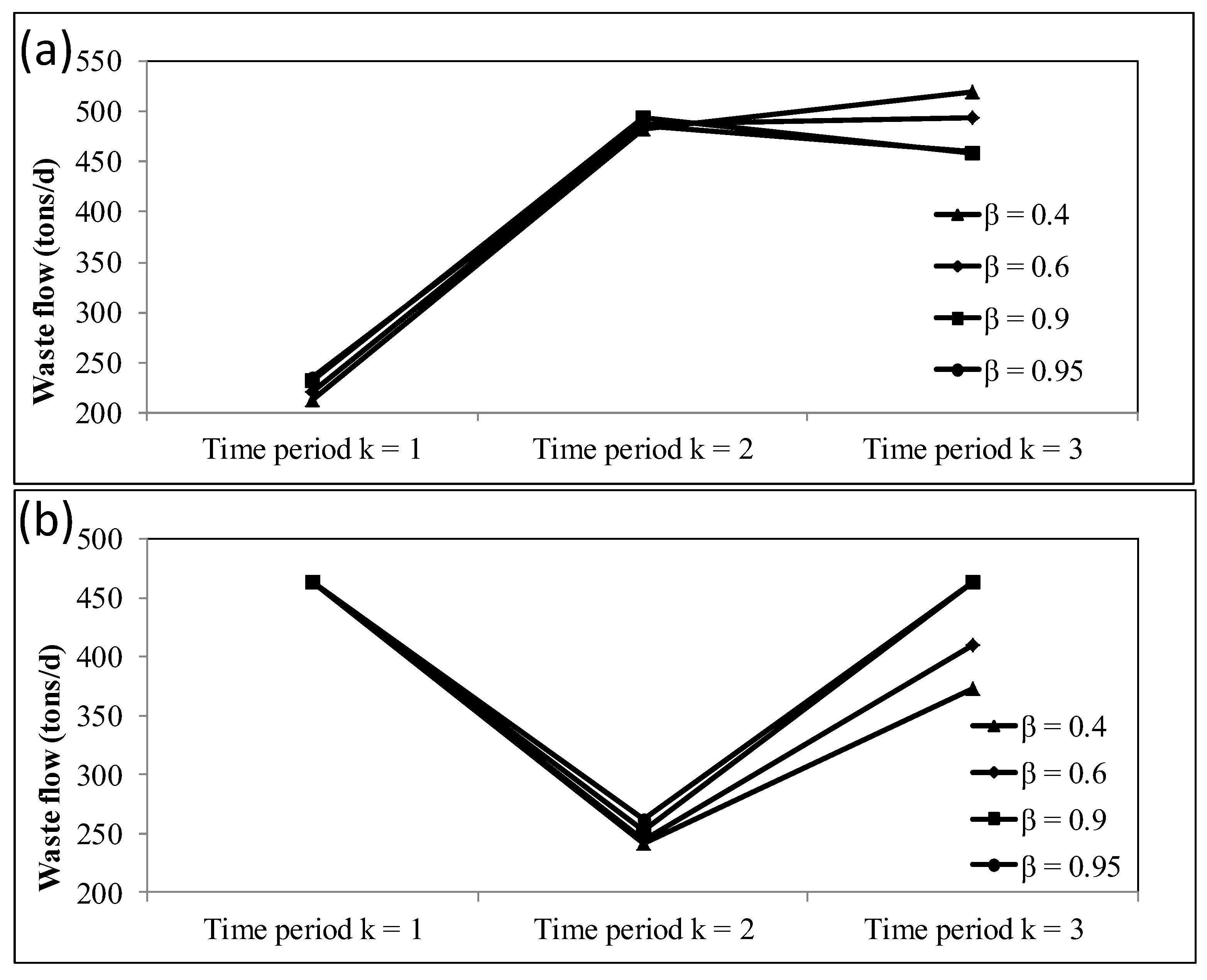
Figure 1 presents the solutions of total allowable waste allocation to facilities under different risk levels ($\beta$). The value of risk level $\beta$ changes from 0.4 to 0.95 under the given specific feasibility degree ${\omega }_1={\omega }_2=0.4$. The results indicate that the total allowable waste allocation would vary significantly because of the variations of risk levels. This means that the violation of the waste-disposal-demand constraint influences the optimized waste flow from cities to facilities. In detail, for waste flow to landfill: the optimized waste flows in time period k = 1 would increase from 212.63 to 234.63 tons/day. The optimized flows in time period k = 2 would increase from 482 to 493.83 tons/day, and then decrease to 485.94 tons/day. The optimized flows in time period k = 3 would decrease from 520.49 to 457.93 tons/day, then increase to 460.78 tons/day. For waste flow to incinerator: the optimized waste flows in time period k = 1 would still stay at 463.37 tons/day. The optimized flows in time period k = 2 would increase from 241 to 261.81 tons/day. The optimized flows in time period k = 3 would increase from 372.61 to 463.37 tons/day.

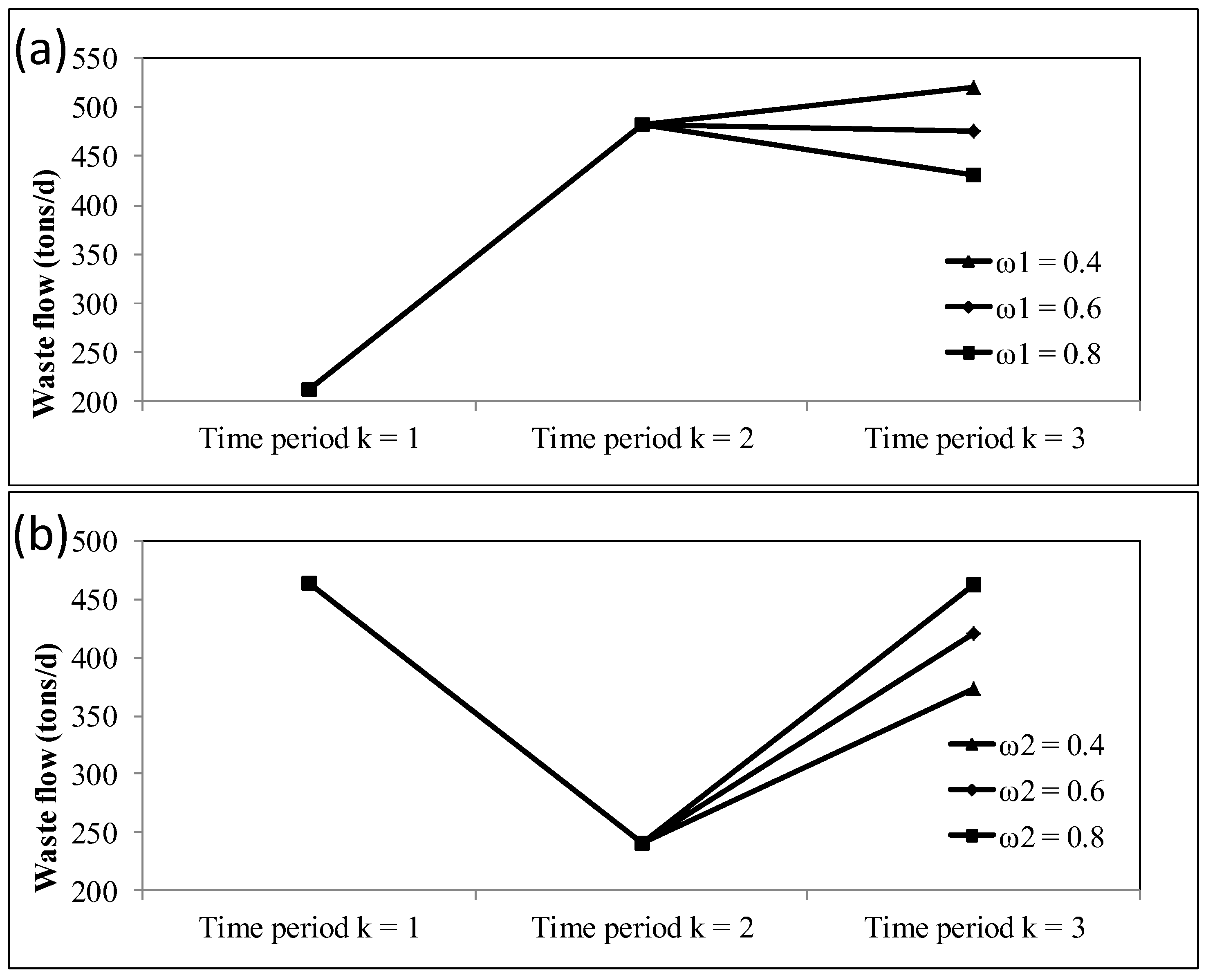
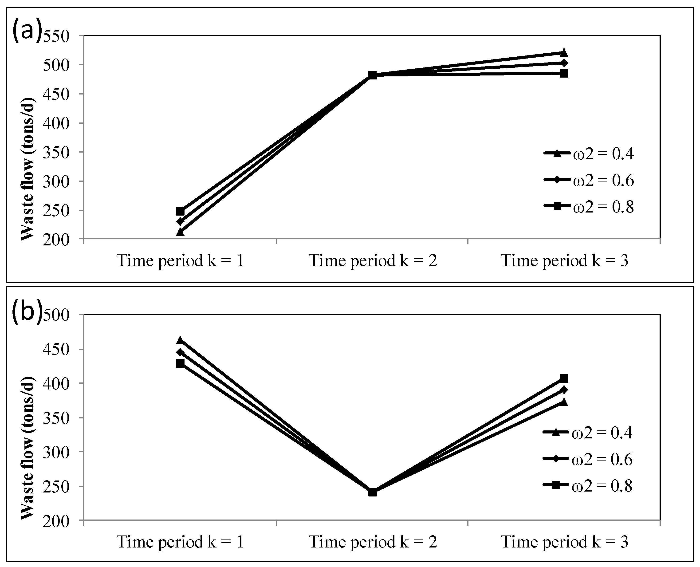
Figure 2 and Figure 3 present the solutions of total allowable waste allocation to facilities under different feasibility degrees ${\omega }_1$ and ${\omega }_2$, respectively. The results indicate that the optimized waste allocation is more sensitive to feasibility degree ${\omega }_2$ than ${\omega }_1$. For example, for larger values of ${\omega }_1$, the amounts of waste to landfill would decrease in time period k = 3, at the same time, the amounts of waste to incinerator would increase in time period k = 3. However, for larger values of ${\omega }_2$, the amounts of waste to landfill would increase in time period k = 1 and decrease in time period k = 3; at the same time, the amounts of waste to incinerator would decrease in time period k = 1 and increase in time period k = 3. Therefore, the effect of vague information in regard to incinerator capacity inputs on waste allocation would be greater.

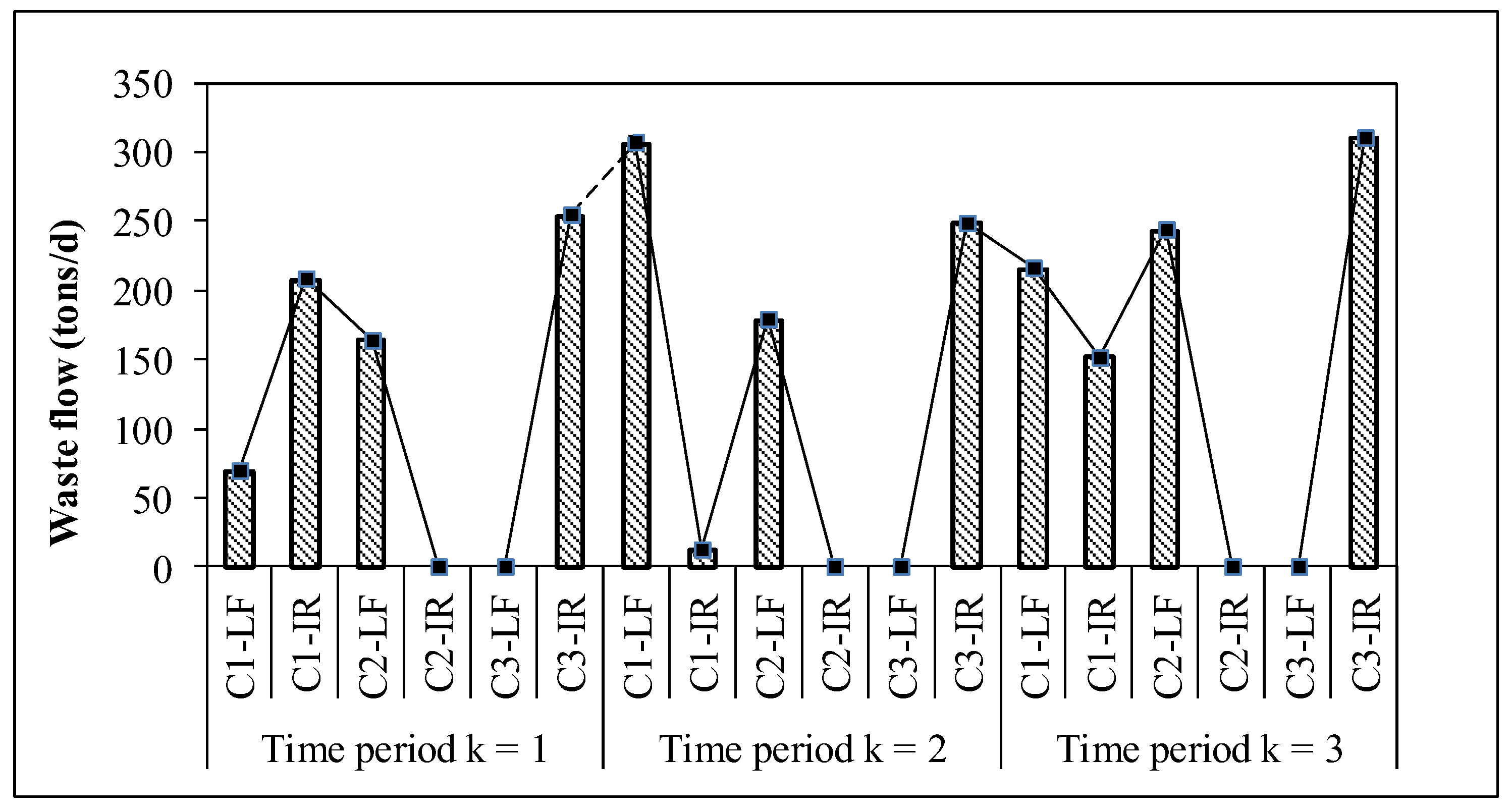
Figure 4 presents the solution generated by the FCVLP model under ${\omega }_1={\omega }_2=0.4$ and $\beta =0.9$. The results show that a reasonable amount of waste flows would be allocated to facilities over three time periods. For example, the waste flows to the landfill and the incinerator from City 1 are 69.88 and 208.62 tons/day in time period k = 1, 306.44 and 12.56 tons/day in time period k = 2, and 216.53 and 151.97 tons/day in time period k = 3, respectively. The waste flows to the landfill from City2 are 164.75, 179.5, and 244.25 tons/day in the three time periods, respectively. There is no waste flow distributed to the incinerator from City 2. The waste flows to the incinerator from City 3 are 254.75, 249.25, and 311.4 tons/day in the three time periods, respectively. There is no waste flow distributed to the landfill from City 3.

The above results demonstrated that FCVLP has the advantages that (1) it can evaluate trade-offs among system cost, feasibility of capacity constraint, and risk of violating the waste-disposal-demand constraint; (2) it can obtain stable solutions of waste flow from cities to facilities; (3) vague information from subjective estimations can be reflected, and MSW managers can identify desired waste management scenarios according to different feasibility degrees and risk levels under uncertainties.

4. Conclusions

In this study, a fuzzy random conditional value-at-risk-based linear programming (FCVLP) method was proposed for municipal solid waste (MSW) management. It can not only deal with uncertainty presented as fuzzy sets, but also tackle problems with respect to trade-offs among the system cost, the risk level of demand constraints, and the feasibility degree of capacity constraints.

In order to demonstrate the applicability of the FCVLP model, a long-term waste management problem was provided. The results indicated that the FCVLP model could generate various plans of waste allocation under various feasibility degrees ($\omega$) and risk levels ($\beta$). The system cost would increase with the increase of risk level $\beta$, which implies that a higher system cost may guarantee that waste disposal demands are met. The system cost would increase with the increase of feasibility degrees ${\omega }_1$ and ${\omega }_2$, which implies that a higher system cost may guarantee that waste facility capacities are met. Moreover, the effects on the system cost from vague information regarding incinerator capacity inputs would be greater than those for landfill capacity inputs.

The total allowable waste allocation would vary significantly because of the variations in risk levels, and the optimized waste allocation is more sensitive to the feasibility degrees of the incinerator-capacity constraints than those of the landfill-capacity constraints.

The study is the first attempt to integrate the FCVaR and FIP methods into a general framework and apply it in solid waste management systems. The proposed method could also be used in other environmental problems under fuzzy random conditions.

References

- Xu, Y.; Huang, G.; Qin, X.; Cao, M. SRCCP: A stochastic robust chance-constrained programming model for municipal solid waste management under uncertainty. Resour. Conserv. Recycl. 2009, 53, 352–363. [Google Scholar] [CrossRef]
- Wang, S.; Huang, G.; Yang, B. An interval-valued fuzzy-stochastic programming approach and its application to municipal solid waste management. Environ. Model. Softw. 2012, 29, 24–36. [Google Scholar] [CrossRef]
- Singh, A.; Basak, P. Economic and environmental evaluation of municipal solid waste management system using industrial ecology approach: Evidence from India. J. Clean. Prod. 2018, 195, 10–20. [Google Scholar] [CrossRef]
- Lu, H.; Huang, G.; He, L.; Zeng, G. An inexact dynamic optimization model for municipal solid waste management in association with greenhouse gas emission control. J. Environ. Manag. 2009, 90, 396–409. [Google Scholar] [CrossRef] [PubMed]
- Gu, B.; Jiang, S.; Wang, H.; Wang, Z.; Jia, R.; Yang, J.; He, S.; Cheng, R. Characterization, quantification and management of China's municipal solid waste in spatiotemporal distributions: A review. Waste Manag. 2017, 61, 67–77. [Google Scholar] [CrossRef]
- Anderson, L.; Nigam, A. A Mathematical Model for the Optimization of a Waste Management System; SERL Report; University of California at Berkeley, Sanitary Engineering Research Laboratory: Berkeley, CA, USA, 1968. [Google Scholar]
- Shekdar, A.V.; Bhide, A.D.; Tikekar, A.G. Optimization of route of refuse transportation vehicles. Indian J. Environ. Health. 1987, 1, 1e15. [Google Scholar]
- Baetz, B.W. Optimization/Simulation Modeling for Waste Management Capacity Planning. J. Fuzzy Plan. Dev. 1990, 116, 59–79. [Google Scholar] [CrossRef]
- Maqsood, I.; Huang, G.H. A Two-Stage Interval-Stochastic Programming Model for Waste Management under Uncertainty. J. Air Waste Manag. Assoc. 2003, 53, 540–552. [Google Scholar] [CrossRef] [PubMed]
- Lu, H.W.; Huang, G.H.; Zeng, G.M.; Maqsood, I.; He, L. An Inexact Two-stage Fuzzy-stochastic Programming Model for Water Resources Management. Water Resour. Manag. 2007, 22, 991–1016. [Google Scholar] [CrossRef]
- Tascione, V.; Mosca, R.; Raggi, A. LCA and linear programming for the environmental optimization of waste management systems: A simulation. In Pathways to Environmental Sustainability; Springer: Cham, Switzerland, 2014; pp. 13–22. [Google Scholar]
- Harijani, A.M.; Mansour, S.; Karimi, B. A multi-objective model for sustainable recycling of municipal solid waste. Waste Manag. Res. 2017, 35, 387–399. [Google Scholar] [CrossRef]
- Huang, G.H.; Baetz, B.W.; Patry, G.G. Grey fuzzy dynamic programming: Application to municipal solid waste management planning problems. Civ. Eng. Syst. 1994, 11, 43–73. [Google Scholar] [CrossRef]
- Chang, N.B.; Wang, S.F. A grey fuzzy multiobjective programming approach for the optimal planning of municipal solid waste management systems. Eur. J. Oper. Res. 1995, 99, 303–321. [Google Scholar] [CrossRef]
- Huang, G.; Sae-Lim, N.; Liu, L.; Chen, Z. An Interval-Parameter Fuzzy-Stochastic Programming Approach for Municipal Solid Waste Management and Planning. Environ. Model. Assess. 2001, 6, 271–283. [Google Scholar] [CrossRef]
- Kanat, G. Municipal solid-waste management in Istanbul. Fuzzy Manag. 2010, 30, 1737–1745. [Google Scholar] [CrossRef] [PubMed]
- Wang, S.; Huang, G. Interactive two-stage stochastic fuzzy programming for water resources management. J. Environ. Manag. 2011, 92, 1986–1995. [Google Scholar] [CrossRef] [PubMed]
- Li, Y.; Huang, G.; Nie, S. A mathematical model for identifying an optimal waste management policy under uncertainty. Appl. Math. Model. 2012, 36, 2658–2673. [Google Scholar] [CrossRef]
- Rajendran, K.; Kankanala, H.R.; Martinsson, R.; Taherzadeh, M.J. Uncertainty over techno-economic potentials of biogas from municipal solid waste (MSW): A case study on an industrial process. Appl. Energy 2014, 125, 84–92. [Google Scholar] [CrossRef] [Green Version]
- Kong, X.; Huang, G.; Fan, Y.; Li, Y. A duality theorem-based algorithm for inexact quadratic programming problems: Application to waste management under uncertainty. Eng. Optim. 2015, 48, 1–20. [Google Scholar] [CrossRef]
- Karagoz, S.; Aydin, N.; Isikli, E. Decision-making in Solid Waste Management under Fuzzy Environment. In Intelligence Systems in Environmental Management: Theory and Applications; Springer International Publishing: Cham, Switzerland, 2017. [Google Scholar]
- Cheng, G.; Huang, G.; Dong, C.; Xu, Y. Distributed mixed-integer fuzzy hierarchical programming for municipal solid waste management. Part I: System identification and methodology development. Environ. Sci. Pollut. Res. 2017, 24, 7236–7252. [Google Scholar] [CrossRef]
- Yadav, V.; Bhurjee, A.; Karmakar, S.; Dikshit, A. A facility location model for municipal solid waste management system under uncertain environment. Sci. Total. Environ. 2017, 603, 760–771. [Google Scholar] [CrossRef]
- Soltani, A.; Sadiq, R.; Hewage, K. The impacts of decision uncertainty on municipal solid waste management. J. Environ. Manag. 2017, 197, 305–315. [Google Scholar] [CrossRef] [PubMed]
- Yano, H.; Sakawa, M. Interactive fuzzy decision making for generalized multiobjective linear fractional programming problems with fuzzy parameters. Fuzzy Sets Syst. 1989, 32, 245–261. [Google Scholar] [CrossRef]
- Huang, G.H.; Baetz, B.W.; Patry, G.G. A Grey fuzzy linear programming approach for municipal solid waste management planning under uncertainty. Civ. Eng. Syst. 1992, 10, 123–146. [Google Scholar] [CrossRef]
- Stanciulescu, C.; Fortemps, P.M.; InstalléWertz, V. Multiobjective fuzzy linear programming problems with fuzzy decision variables. Eur. J. Oper. Res. 2003, 149, 654–675. [Google Scholar] [CrossRef]
- Wang, H.-F.; Wu, K.-Y. Preference Approach to Fuzzy Linear Inequalities and Optimizations. Fuzzy Optim. Mak. 2005, 4, 7–23. [Google Scholar] [CrossRef]
- Xu, J.; Fang, H.; Zhou, T.; Chen, Y.-H.; Guo, H.; Zeng, F. Optimal robust position control with input shaping for flexible solar array drive system: A fuzzy-set theoretic approach. IEEE Trans. Fuzzy Syst. 2019. [Google Scholar] [CrossRef]
- Zhang, X.; Huang, G.H.; Chan, C.W.; Liu, Z.; Lin, Q. A fuzzy-robust stochastic multiobjective programming approach for petroleum waste management planning. Appl. Math. Model. 2010, 34, 2778–2788. [Google Scholar] [CrossRef]
- Fan, Y.R.; Huang, G.H.; Veawab, A. A generalized fuzzy linear programming approach for environmental management problem under uncertainty. J. Air Waste Manag. Assoc. 2012, 62, 72–86. [Google Scholar] [CrossRef]
- Fan, Y.; Huang, G.; Yang, A. Generalized fuzzy linear programming for decision making under uncertainty: Feasibility of fuzzy solutions and solving approach. Inf. Sci. 2013, 241, 12–27. [Google Scholar] [CrossRef]
- Fan, Y.; Huang, G.; Jin, L.; Suo, M. Solid waste management under uncertainty: A generalized fuzzy linear programming approach. Civ. Eng. Environ. Syst. 2014, 31, 331–346. [Google Scholar] [CrossRef]
- Nasseri, S.H.; Zavieh, H. A Multi-objective Method for Solving Fuzzy Linear Programming Based on Semi-infinite Model. Fuzzy Inf. Eng. 2018, 10, 91–98. [Google Scholar] [CrossRef] [Green Version]
- Linsmeier, T.J.; Pearson, N.D. Value at Risk. Financ. Anal. 2000, 56, 47–67. [Google Scholar] [CrossRef]
- Quaranta, A.G.; Zaffaroni, A. Robust optimization of conditional value at risk and portfolio selection. J. Bank. Finance 2008, 32, 2046–2056. [Google Scholar] [CrossRef]
- Jin, P. Value at risk and tail value at risk in uncertain environment. In Proceedings of the Eighth International Conference on Information and Management Sciences, Kunming, China, 20 July 2009. [Google Scholar]
- Liu, B. Uncertainty Theory; Springer: Berlin, Germany, 2007. [Google Scholar]
- Rockafellar, R.; Uryasev, S. Conditional value-at-risk for general loss distributions. J. Bank. Finance 2002, 26, 1443–1471. [Google Scholar] [CrossRef]
- Jiménez, M.; Arenas, M.; Bilbao, A.; Rodrı´guez, M.V. Linear programming with fuzzy parameters: An interactive method resolution. Eur. J. Oper. Res. 2007, 177, 1599–1609. [Google Scholar] [CrossRef]
Figure 1.
Total waste flow to facilities under different levels when : (a) to landfill; (b) to incinerator.
Figure 2.
Total waste flow to facilities under different degrees when : (a) to landfill; (b) to incinerator.
Figure 3.
Figure 4.
Waste flow from cities to facilities under , (where C1, C2, and C3 represent cities; and LF and IR represent the landfill and the incinerator, respectively. There are 18 conditions including C1-LF on k = 1, C1-IR on k = 2, and so on).