The Impact of the East Atlantic/Western Russia Pattern on the Hydroclimatology of Europe from Mid-Winter to Late Spring

Abstract

In this study, the influence of the East Atlantic/Western Russia teleconnection pattern on the hydroclimatology of Europe, from mid-winter to late spring, is investigated. The influence of EAWR on the variability of precipitation (PP), temperature (TT) and standardized precipitation-evapotranspiration index (SPEI) is investigated on the base of correlation and stability maps. It is shown that EAWR has a strong impact on the coupling between the sub-tropical Atlantic Jet and the African Jet, which in turn affects the climate variability over Europe from mid-winter to late spring. The strongest impact of the mid-winter EAWR over the European precipitation is found to be in mid-winter and early spring over the northern part of the Scandinavian Peninsula and the central and eastern part of Europe; while the influence of the mid-winter EAWR on European temperature persists from mid-winter to late spring, giving the possibility of a potential predictability for spring temperature over extended European regions.

1. Introduction

The global atmospheric circulation has a number of preferred patterns of variability, all of which have expressions in surface climate. Monthly mean surface pressure varies markedly about the long-term mean sea level pressure (SLP) distribution. This variability occurs in well-defined spatial patterns [1,2] particularly during the boreal winter over the Northern Hemisphere (NH). Such variations are commonly referred as “teleconnections” in the literature, since they result in simultaneous variations in weather and climate over widely separated points over the earth. Regional climates in different locations may vary out of phase, owing to the action of such teleconnections, which modulate the location and strength of the storm tracks and poleward fluxes of heat, moisture and momentum [3,4,5]. Such monthly, seasonal and longer-time scales anomalies have direct impacts on humans, as they are often associated with floods, droughts, heat or cold waves and other factors that can directly affect and disrupt agriculture, water supplies, and can modulate the fresh water quality, energy demands and human health. The strength of these teleconnections and the way they influence surface climate variables varies over long time scales [1,2,3].

The climate over the European region is dominated by the North Atlantic Oscillation (NAO) [3,6]. NAO is the leading mode of climate variability in the North Atlantic region and is characterized by a meridional seesaw in the atmospheric pressure between the Icelandic Low and the Azores High. Periods with positive values of the NAO index are characterized by an enhanced westerly flow across the North Atlantic and the European region and higher than normal surface pressure south of 55°N combined with a broad region of anomalously low pressure throughout the Arctic and subarctic. Consequently, this phase is associated with stronger-than-average winds across the mid-latitudes of the Atlantic onto Europe, with anomalously southerly flow over the eastern United States and anomalously northerly flows across Greenland, the northern part of Canada and the Mediterranean region and enhanced easterly trade winds over the sub-tropical North Atlantic [7]. Although NAO is one of the most prominent teleconnection patterns in all seasons [2], its relative role in regulating the variability of the European climate during non-winter months is not as clear as for the winter season. At the same time, the mechanisms which drive the European climate variability might vary from one climatic period to another and also might be different for different variables (e.g., precipitation, streamflow, air temperature).

Another prominent teleconnections pattern over the North Atlantic region is the East Atlantic—West Russia (EAWR). The EAWR was originally identified through an orthogonally rotated principal component analysis (RPCA) applied to the monthly-mean geopotential height at 700 hPa and consists of four main anomaly centers [2]. The positive phase is associated with positive height anomalies located over Europe and northern China, and negative height anomalies located over the central North Atlantic and north of the Caspian Sea. During the positive (negative) phase of the EAWR, wetter (drier) conditions are observed over eastern China and drier (wetter) conditions prevail across central Europe and the Mediterranean Region. The positive (negative) phase of EAWR is also associated with above-average (below-average) temperatures over eastern Asia and below-average (above-average) temperatures over western Russia and northeastern Africa [2].

EAWR was found to have a strong influence over the precipitation in the Mediterranean region [8,9]. According to the aforementioned studies, extreme wet (dry) winter months over the Mediterranean region were characterized by anomaly patterns which project onto the negative (positive) phase of EAWR. A strong relationship between EAWR and the temperature variability inside a cave from the north-western part of Romania has also been found [10]. High (low) temperatures inside the cave are associated with an atmospheric circulation that resembles the center of action of the EAWR pattern [11] found that both NAO as well as EAWR play a significant role on the variability of cyclones and wind activity over the Mediterranean region. According to the aforementioned study, during the positive phase of EAWR, the storm numbers over the central Mediterranean region are decreasing and the number of strong wind events over the eastern Mediterranean region is increasing.

Although EAWR is one of the dominant modes of variability over the North Atlantic—Eurasian region, less attention has been paid to the role of the EAWR pattern on the European climate. As shown in the previous paragraph, most of the existing studies are focused over the Mediterranean region or they reflect the influence of EAWR on the cyclonic activity, storminess and wind events. Based on the aforementioned studies, it is clear that EAWR has a strong influence on the climatic conditions over Europe, especially the central and southern part. Motivated by this, the aim of the current study is to investigate the possible influence of EAWR pattern over the European hydroclimatology, in terms of seasonal precipitation, temperature and dry/wet conditions, from mid-winter to early spring and indentify a potential predictive skill for European hydroclimatology based on the EAWR index. The paper is organized in four sections. In Section 2, the data and methods employed in this study are described. In Section 3 the relationship between EAWR index and the large-scale atmospheric circulation and precipitation, temperature and dry/wet periods is investigated. A possible mechanism by which EAWR can affect the climate over Europe is given and the stationarity of the relationship between EAWR and precipitation, temperature and drought conditions over Europe is tested. The main conclusions follow in Section 4.

2. Data and Methodology

The seasonal January–February–March (JFM) EAWR index values were extracted from [12]. The procedure used to identify the Northern Hemisphere teleconnection patterns, including EAWR is the Rotated Principal Component Analysis [2]. The JFM time series, used in this study, covers the period 1950–2012.

In order to analyze the temporal structure (interannual and decadal variability) of the EAWR index variability the wavelet power spectrum analysis was used. The wavelet analysis used in this paper follows the methods of [13]. Statistical significance is determined against a red noise null hypothesis using a chi-squared test. By decomposing a time series into a time-frequency space, it is possible to determine the dominant modes of variability and how these modes vary in time. For the precipitation (PP) and temperature (TT), we made use of the updated CRU T.S 3.20 data set [14], for the period 1950–2012. This data set provides monthly values for various parameters for the global land areas. The temporal coverage is 1901–2012 on a 0.5° × 0.5° grid. To quantify the meteorological drought we used the newly developed Standardized Precipitation Evapotranspiration Index (SPEI). SPEI is a multi-scalar drought indicator and is based on monthly precipitation totals and temperature means and uses a simple approach to calculate the Potential Evapotranspiration (PET) [15]. SPEI is similar to the Standardized Precipitation Index [16], but it includes the role of temperature. For calculating the SPEI we used the algorithm developed by [15] and we used the precipitation and potential evapotranspiration data from on the CRU T.S. 3.20 dataset [14]. In this study we employ SPEI for one accumulation period of 3 months. SPEI3 was calculated for each month of the year, but for this study we used just the seasonal means of January–February–March (JFM), February–March–April (FMA) and March–April–May (MAM), respectively. The estimation of PET is based on the Penmann-Monteith method [15].

For the Northern Hemisphere atmospheric circulation we use the geopotential height at 500 hPa (Z500) and the zonal mean wind at 200 hPa (U200), on a 2.5° × 2.5° grid from the NCEP/NCAR data [17], for the period 1950–2012. The vertically integrated water vapor transport (WVT) [18] is calculated through zonal wind (u), meridional wind (v) and specific humidity (q), from the same data set [17]. WVT vectors for latitude (ϕ) and longitude (λ) are defined as follows:

(1)

where zonal (Q_λ) and meridional (Q_Ф) components of Q are given by Equation (2):

(2)

For each vertical layer and each grid-point we calculate the product between the monthly values of horizontal wind and specific humidity (q). The result is multiplied with the pressure thickness of the layer they represent and divided by gravity. The WVT is obtained by summation of water transport for all layers located between the earth’s surface and 300 hPa level. We also used the divergence of water vapor K, which is in balance with the surface fresh water flux E − P [17]:

(3)

where ∇ denotes the two dimensional divergence operator, E evaporation and P precipitation. Regions of mean positive divergence (E − P > 0) constitute source regions of water vapor, meanwhile the regions of convergence (E − P < 0) are sink regions for water vapor.

To assess the link between EAWR index and large scale atmospheric circulation we have constructed the composite maps of Z500, U200, WVT, the velocity potential and divergent wind at 200 hPa and 850 hPa, respectively. The composite maps are defined by average fields of Z500, U200, WVT, the velocity potential and divergent wind at 200 hPa and 850 hPa for the years when the JFM EAWR index was higher (lower) than 1 (−1) standard deviation. This threshold was chosen as a compromise between the strength of the climate anomalies associated to flow anomalies and the number of maps which satisfy this criteria. Further analysis has shown that the results are not sensitive to the exact threshold value used for our composite analysis (not shown). For Z50, the velocity potential and divergent wind at 200 hPa and 850 hPa, just the difference between High (EAWR JFM > 1 standard deviation)—Low (EAWR JFM < −1 standard deviation) composite maps is shown. The level of significance of the composite maps is established by means of a Student’s t test [19].

In order to establish the stationarity of the relationship between EAWR index and PP, TT and SPEI3 fields over Europe, we apply the methodology used for river streamflow forecast [11,20,21] namely the stability maps. The aim of this method is to find regions where the correlation between the variables remains stable in time, after applying a correlation in a 21 years moving window. The correlation is considered to be stable for the grid points where the JFM EAWR index and the PP, TT and SPEI3 field are significantly correlated at the 90% level (r = 0.24) or 80% (r = 0.17) for more than 80% of the 21 year windows covering the period 1950–2012. A more detailed description of the method can be found in [20,22].

3. Results

3.1. Time Series Analysis

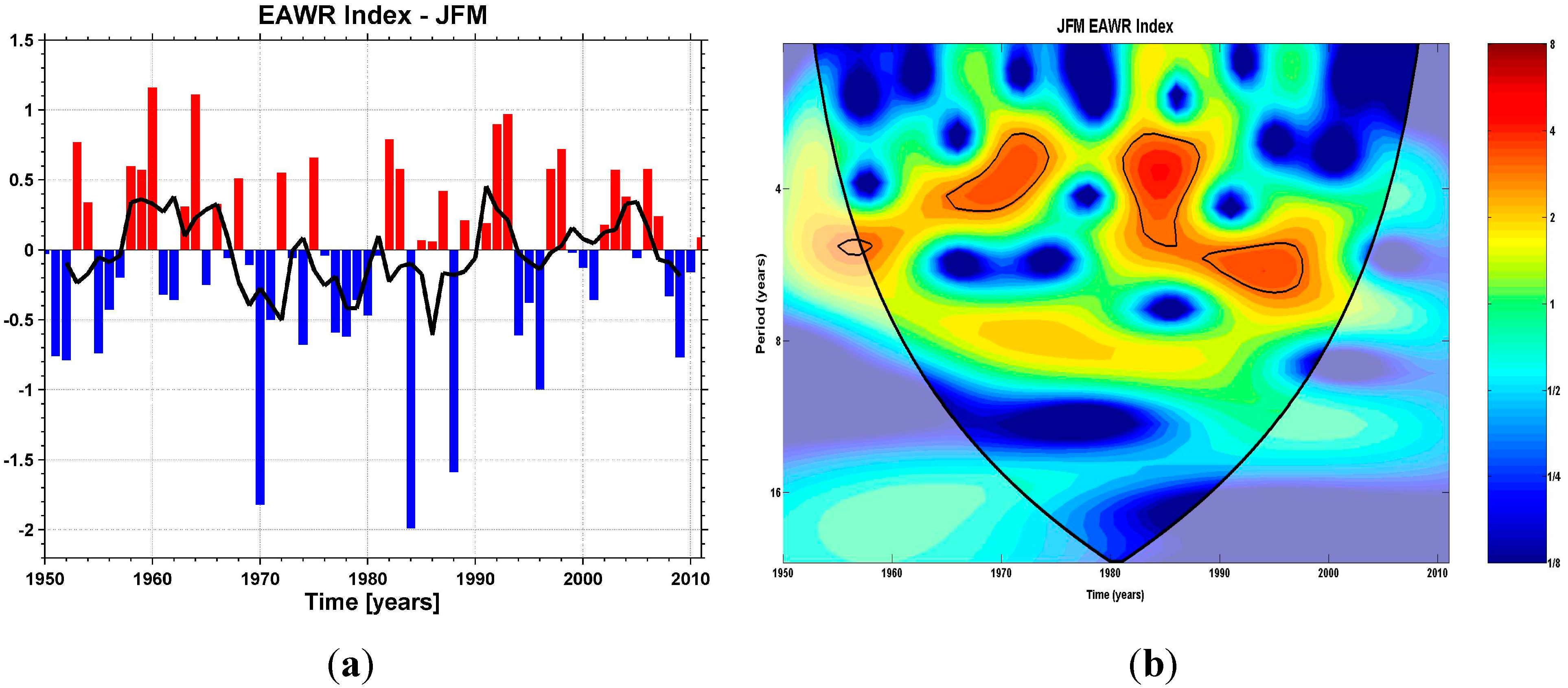
The temporal evolution of the EAWR index, for the period 1950–2012, is shown in Figure 1a. The time series of JFM EAWR index presents pronounced interannual variability and higher amplitude for the negative phase. Persistent negative anomalies were observed during the mid-winters of 1970, 1977 and 1979, periods which were also characterized by enhanced precipitation over the western part of Europe (Figure 1a). The wavelet analysis reveals a significant periodicity in the 2–6 years band (Figure 1b) and a weaker periodicity at around 8 years. The Morlet wavelet spectrum (Figure 1b) of the JFM EAWR index shows a nonstationary behavior, especially in the 2–6 years band. This nonstationary behavior emphasizes the fact that the strength of the interannual variability of the JFM EAWR index has varied with time.

Figure 1. (a) Annual January to March (JFM) value of the East Atlantic/Western Russia (EAWR) Index and the 5 years running mean (black line); (b) The continuous wavelet power spectrum of the time series of JFM EAWR Index. The thick black line contour is the 5% significance level against red noise.

Figure 1. (a) Annual January to March (JFM) value of the East Atlantic/Western Russia (EAWR) Index and the 5 years running mean (black line); (b) The continuous wavelet power spectrum of the time series of JFM EAWR Index. The thick black line contour is the 5% significance level against red noise.

3.2. Relationship of the EAWR with the Atmospheric Circulation

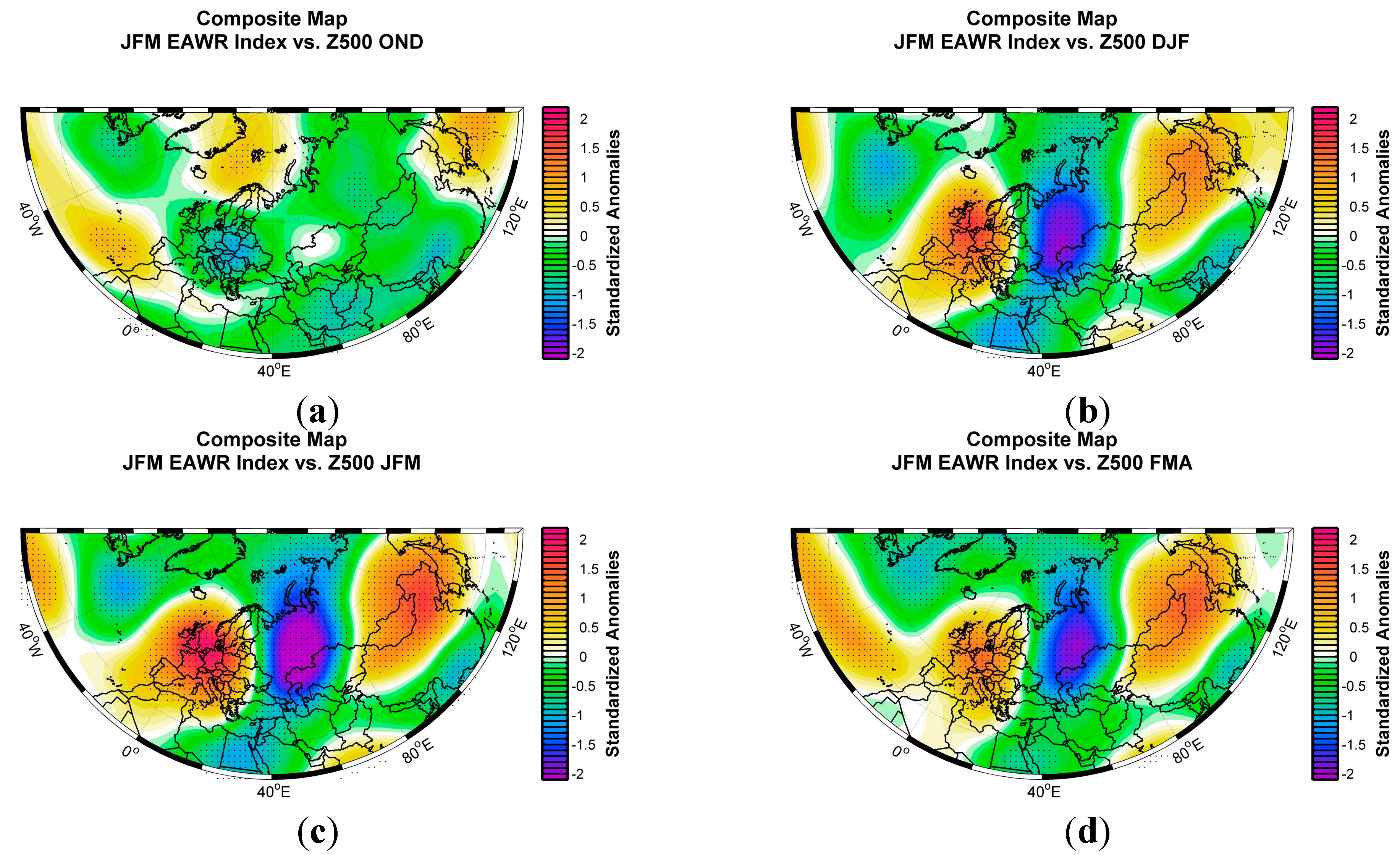
The relationship between the JFM EAWR index and geopotential height at 500 hPa is investigated using lagged composite maps. The use of lagged composite makes it possible to detect the prior development and subsequent decay of Z500 anomalies associated with the JFM EAWR structure. Here we use seasonal anomalies for Z500 defined as: October–November–December (OND), December–January–February (DJF) and February–March–April (FMA)). The seasonal anomalies were calculated by subtracting mean annual cycle. After that the long-term mean of every calendar month was subtracted from each individual month and the seasonal anomalies were calculated as 3-month averages. To obtain the normalized anomalies all the data sets employed were normalized by their standard deviation.

There is little EAWR signature in the 500-hPa geopotential height anomalies during the late autumn and early-winter (OND) (Figure 2a). By mid-winter (DJF), the classic EAWR pattern starts to develop, particularly over Europe and eastern Russia (Figure 2b). There are significant 500 hPa height anomalies over Europe and the Scandinavian Peninsula, negative anomalies over eastern Russia and positive anomalies over northern part of China and Mongolia. By late winter, the geopotential height anomalies pattern becomes more pronounced and all the centers of action characteristic to the EAWR pattern become much stronger (Figure 2c). During late spring (February–April), the overall geopotential height anomalies related to EAWR persist, but their intensity decreases (Figure 2d).

Figure 2. Geopotential Height at 500 hPa composite map (difference between the averaged maps for which the EAWR JFM index was higher (lower) than 1 (–1) standard deviation) for (a) October to December (OND); (b) December to February (DJF) (c) January to March (JFM) and (d) February to April (FMA). Hatching displays areas at or over 95% sign significance level using a two tailed t-test.

Figure 2. Geopotential Height at 500 hPa composite map (difference between the averaged maps for which the EAWR JFM index was higher (lower) than 1 (–1) standard deviation) for (a) October to December (OND); (b) December to February (DJF) (c) January to March (JFM) and (d) February to April (FMA). Hatching displays areas at or over 95% sign significance level using a two tailed t-test.

3.3. TheInfluence of EAWM on the Hydroclimatology over the European Region

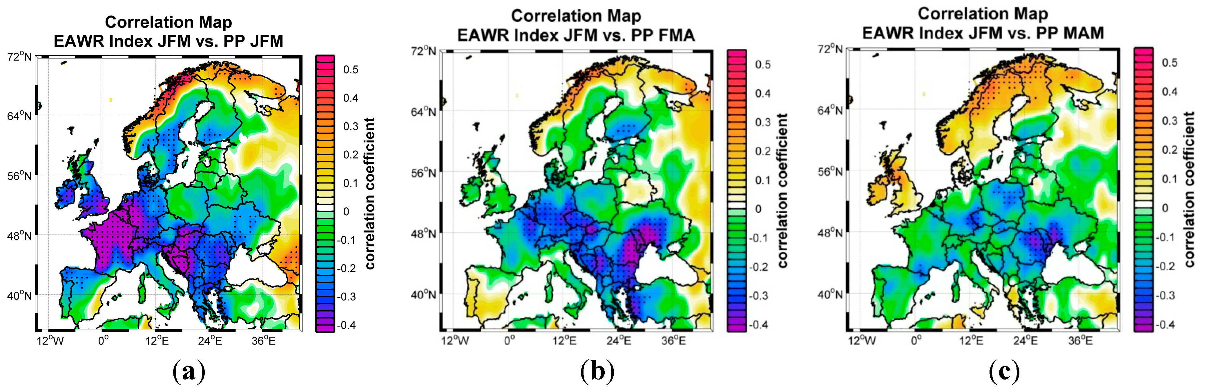
The relationship between JFM EAWR and PP, TT and SPEI3 over Europe, is investigated using lagged correlation maps, with JFM EAWR index leading the aforementioned fields. The seasonal averages of PP, TT and SPEI3 were computed in a similar way as for Z500. For PP, TT and SPEI3 we used seasonal averages for the following seasons: January–February–March (JFM), February–March–April (FMA) and March–April May (MAM).

Positive EAWR phase is typically associated with wetter than normal conditions over the western coast of the Scandinavian Peninsula and drier than normal conditions over central Europe and the Balkans (Figure 3a). In early spring (Figure 3b) the EAWR influence remains significant just over the central and the eastern part of Europe. In late spring the influence of EAWR persists over the eastern part of Europe and over the northern part of the Scandinavian Peninsula (Figure 3c). As it can be inferred from Figure 3a–c there is a propagation of the influence of EAWR on the European precipitation from the west towards east, from mid-winter towards late spring.

Figure 3. Correlation between the JFM EAWR and CRU T.S. 3.2 Precipitation (PP) for (a) January to March (JFM); (b) February to April (FMA) and (c) March to May (MAM). Hatching displays areas at or over 95% significance level using a two tailed t-test.

Figure 3. Correlation between the JFM EAWR and CRU T.S. 3.2 Precipitation (PP) for (a) January to March (JFM); (b) February to April (FMA) and (c) March to May (MAM). Hatching displays areas at or over 95% significance level using a two tailed t-test.

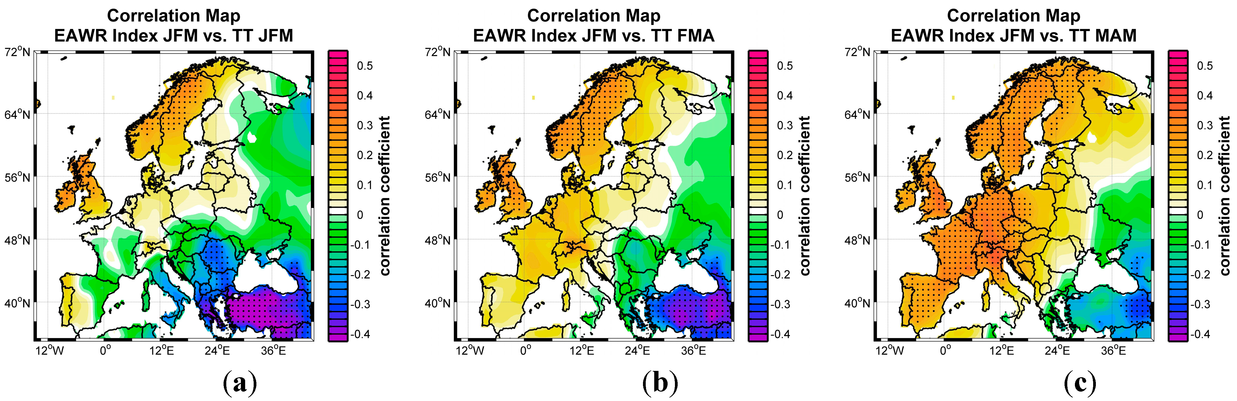
Mid-winter temperatures during the positive phase of EAWR are characterized by warmer than normal conditions over the Scandinavian Peninsula and colder than average conditions over the Balkan region. Outside these regions the correlation is low and insignificant (Figure 4a). For the early spring the positive anomalies persist and they are as significant and extended as in the case of mid-winter (Figure 4b). Furthermore, the influence of EAWR starts to be seen also on the temperature over the central Europe. By late spring the warmer than normal conditions are prevailing mostly over the central part of Europe and the Scandinavian Peninsula (Figure 4c), remaining significant at the 95% level. The influence over the Balkan regions starts to disappear. As in the case of precipitation, there is also a north-west to south-east propagation of the influence of EAWR on the European temperature, from mid-winter to late spring.

Figure 4. Correlation between the JFM EAWR and CRU T.S. 3.2 Temperature (TT) for (a) January to March (JFM); (b) February to April (FMA) and (c) March to May (MAM). Hatching displays areas at or over 95% significance level using a two tailed t-test.

Figure 4. Correlation between the JFM EAWR and CRU T.S. 3.2 Temperature (TT) for (a) January to March (JFM); (b) February to April (FMA) and (c) March to May (MAM). Hatching displays areas at or over 95% significance level using a two tailed t-test.

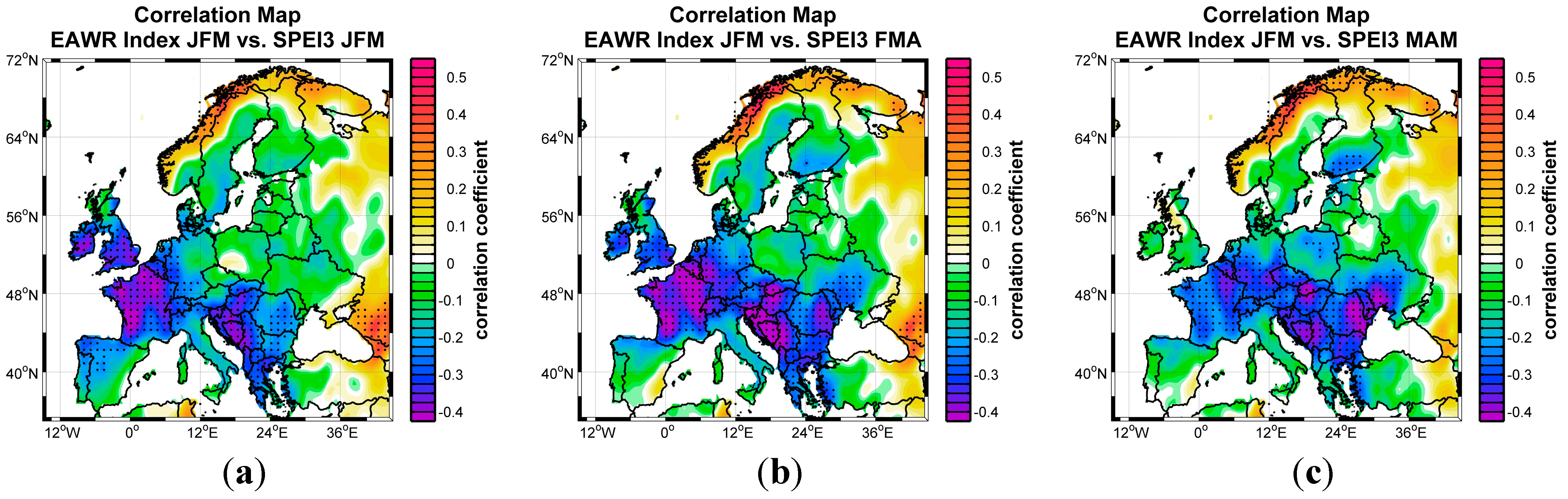
The influence of EAWR pattern on the occurrence of mid-winter droughts follows the same path as precipitation (Figure 5a), but for some regions the correlations are higher (e.g., the eastern part of Europe). This can be due to the fact that SPEI integrates information from PP as well as TT. During the positive phase of EAWR most of the European regions are exposed to meteorological drought, while the northern part of the Scandinavian Peninsula is characterized by wet conditions. In early spring the correlation between the JFM EAWR index and FMA SPEI3 becomes higher over the European region (Figure 5b), meaning that the influence of mid-winter EAWR has a stronger impact over the central Europe in the upcoming early spring. For the late spring (Figure 5c), the influence of EAWR persists over the same regions, but the correlation decreases over the central part of Europe, but remains still significant at 95% level.

Figure 5. Correlation between the JFM EAWR and SPEI3 for (a) January to March (JFM); (b) February to April (FMA) and (c) March to May (MAM). Hatching displays areas at or over 95% significance level using a two tailed t-test.

Figure 5. Correlation between the JFM EAWR and SPEI3 for (a) January to March (JFM); (b) February to April (FMA) and (c) March to May (MAM). Hatching displays areas at or over 95% significance level using a two tailed t-test.

3.4. Physical Mechanism

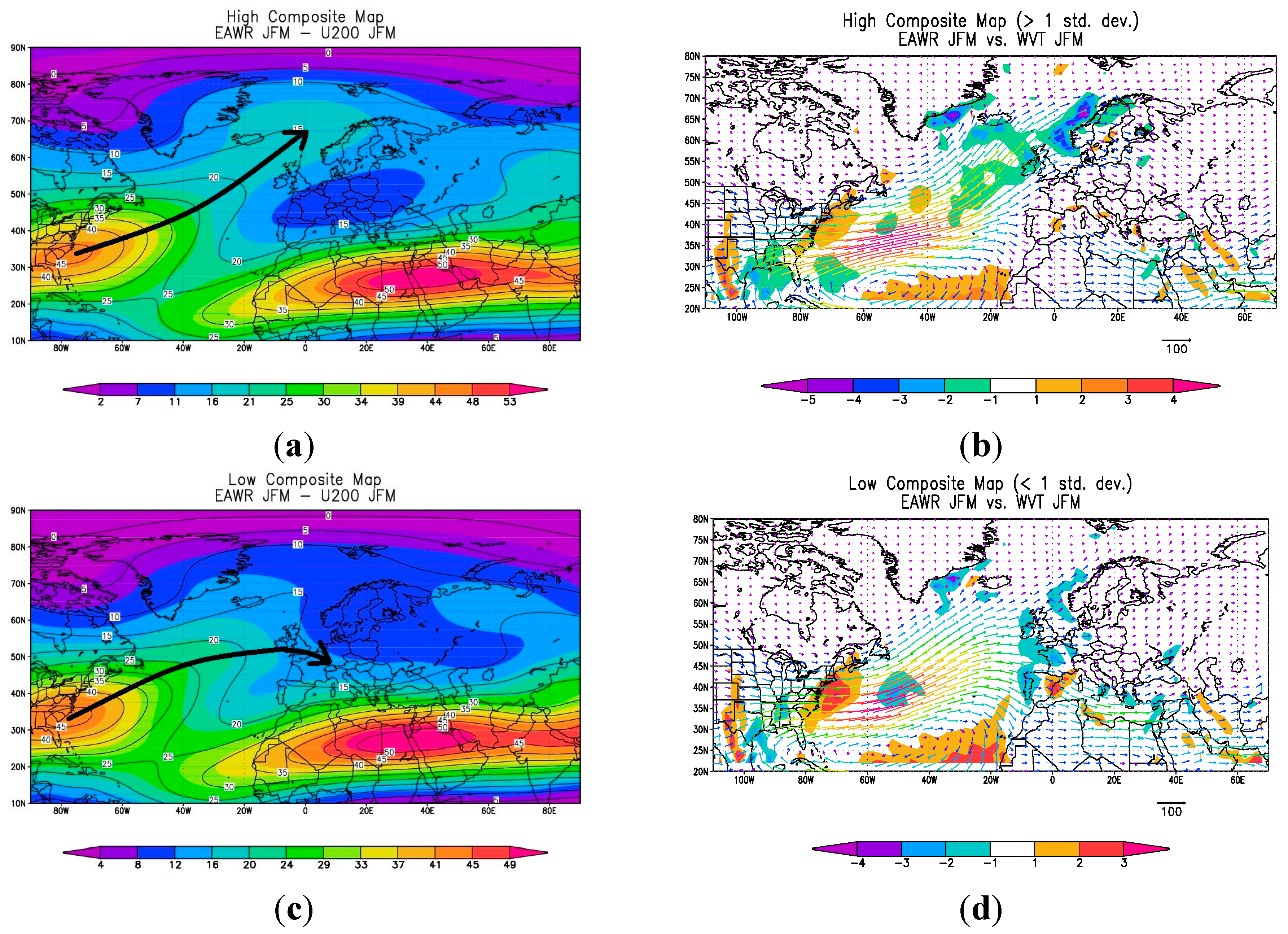
To identify the physical mechanism by which EAWR influences the hydroclimatology variability over Europe, we constructed the composite maps between the normalized and standardized time series of EAWR JFM and the seasonal average (JFM) of the zonal component of mean wind at 200 hPa (U200) and the vertically integrated water vapor transport (WVT), for the years of high (>1 standard deviation) and low (<−1 standard deviation) values of the normalized EAWR index. As in the case of Z500, this threshold was chosen as a compromise between the strength of climate anomalies associated with EAWR and the number of maps that satisfy this criterion.

As it can be inferred from Figure 6 a pronounced difference is found in the structure of the near-tropopause Atlantic subtropical jet, represented here by the averaged seasonally magnitude of the 200 hPa wind vector. During the positive phase of EAWR the degree of separation between the Atlantic and the North African segment of the subtropical jet is considerably more pronounced (Figure 6a), comparative to the negative phase of EAWR (Figure 6b). As a consequence, during the positive phase of EAWR, the central and southern part of Europe is characterized by dry conditions (see Figure 3a), while the northern part of the Scandinavian Peninsula is characterized by wet conditions due to the fact that the jet exit points towards Scandinavia (Figure 6a). According to [23] the poleward side of the jet exit regions is preferred for cyclonic growth, which in turn can induce a large amount of precipitation. During the negative phase of EAWR the axis of the Atlantic Jet is shifted southward and the two jets are almost coupled (Figure 6b). In this case, the western part of Europe receives more precipitation than normal, being situated to the west side of the jet exit.

Figure 6. The composite maps between the normalized time series of JFM EAWR and JFM zonal component of mean wind at 200 hPa for (a) High (JFM EAWR > 1 std. dev.) and (c) Low (JFM EAWR < −1 std. dev.) The composite maps between the normalized time series of JFM AO and JFM vertically integrated water vapor transport for (b) High (JFM EAWR > 1 std. dev.) and (d) Low (JFM EAWR < −1 std. dev.) For (a,c) Climatological means are shown as contour lines. Units are m/s; For (b,d): The shaded areas indicate the distribution of the horizontal divergence of the total water vapor transport (units 10⁻⁶ kg/m²s).

Figure 6. The composite maps between the normalized time series of JFM EAWR and JFM zonal component of mean wind at 200 hPa for (a) High (JFM EAWR > 1 std. dev.) and (c) Low (JFM EAWR < −1 std. dev.) The composite maps between the normalized time series of JFM AO and JFM vertically integrated water vapor transport for (b) High (JFM EAWR > 1 std. dev.) and (d) Low (JFM EAWR < −1 std. dev.) For (a,c) Climatological means are shown as contour lines. Units are m/s; For (b,d): The shaded areas indicate the distribution of the horizontal divergence of the total water vapor transport (units 10⁻⁶ kg/m²s).

To further prove that the jet axis plays a crucial role in the variability of the climate over Europe we have applied the same analysis (composite maps) to the field of WVT. The WVT is strongly related with the Jet variability. In the exit regions of the Atlantic Jet a meridional circulation carries negative vorticity southward in the upper troposphere and the return branch of this circulation enhances the baroclinicity on the lower troposphere through the northern thermal advection. During the positive phase of EAWR (Figure 6c), the axis of the maximum transport is directed towards Scandinavia and there is a significant reduction of the water vapor transport from the Atlantic towards Europe. In the same time a convergent zone develops over the northern part of the Scandinavian Peninsula, which in turn enhances precipitation. The path of the axis of WVT follows the same direction as the Atlantic Jet axis. During the negative phase of EAWR the axis of the WVT is directed towards Europe (Figure 6d), enhancing precipitation over the western and southern part of Europe (in agreement with Figure 3b) due to the convergent zones which are developing.

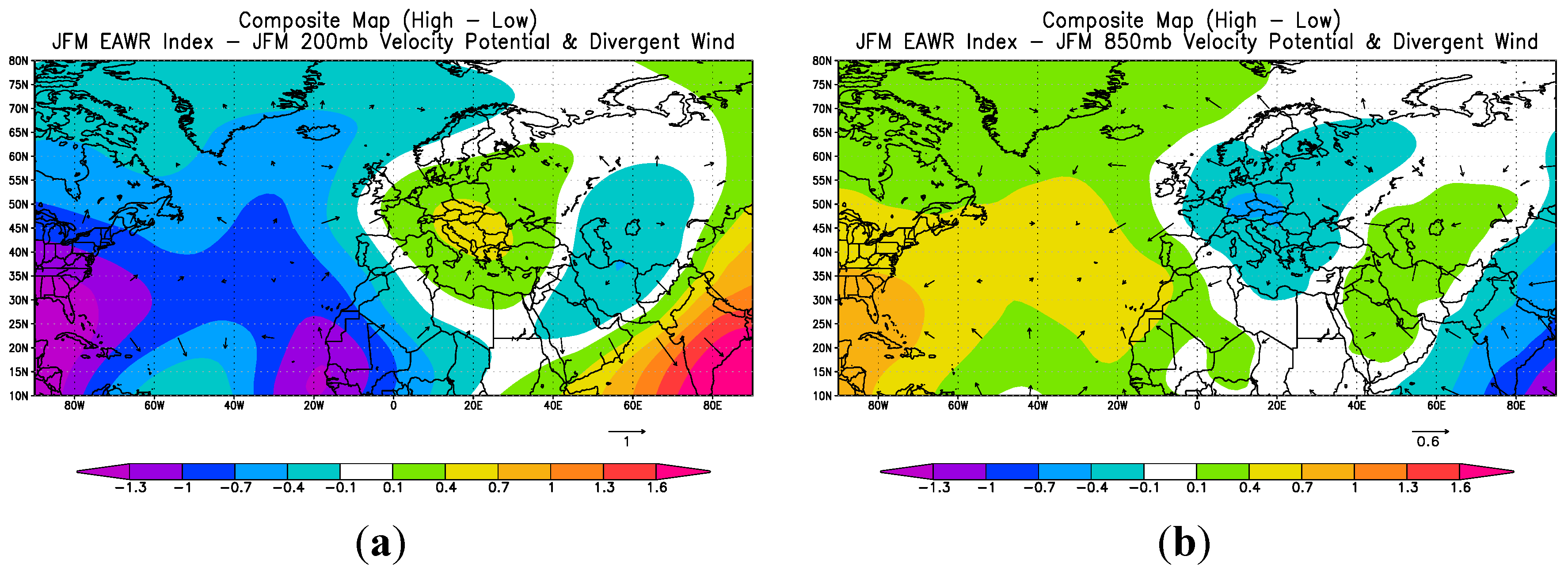
To support this idea we have plotted the composite maps between the EAWR JFM index and the 200 hPa and 850 hPa velocity potential and the divergent wind (Figure 7). At upper levels, during the positive phase of EAWR, there is a well organized zonal quadruple structure over the Atlantic Ocean, central and southern part of Europe, Caspian Sea and India (Figure 7a). At 200 hPa level there is a region of positive velocity potential anomalies over the central and southern part of Europe, which means convergent winds at upper levels and divergent winds at lower levels (Figure 7b) over these areas, flanked (at 200 hPa level) by two regions of convergence over the Atlantic Ocean and one over the Caspian Sea. Based on Figure 7, during the positive phase of EAWR, the central Europe is characterized by surface divergence and upper-levels convergence, meaning subsiding air over central Europe and reduced precipitation. This is in agreement with the results from Figure 3 and Figure 4, respectively, based on which, during the positive phase of EAWR the central and southern part of Europe are characterized by higher than normal temperatures and reduced precipitation.

Figure 7. (a) 200 hPa velocity potential (shaded) and divergent wind (wind bars) composite map (difference between the averaged maps for which the normalized EAWR JFM index was higher (lower) than 1 (−1) standard deviation); (b) 850 hPa velocity potential (shaded) and divergent wind (wind bars) composite map (difference between the averaged maps for which the normalized EAWR JFM index was higher (lower) than 1 (−1) standard deviation). Units are: 10⁶ m²/s for the velocity potential and m/s for the divergent wind.

Figure 7. (a) 200 hPa velocity potential (shaded) and divergent wind (wind bars) composite map (difference between the averaged maps for which the normalized EAWR JFM index was higher (lower) than 1 (−1) standard deviation); (b) 850 hPa velocity potential (shaded) and divergent wind (wind bars) composite map (difference between the averaged maps for which the normalized EAWR JFM index was higher (lower) than 1 (−1) standard deviation). Units are: 10⁶ m²/s for the velocity potential and m/s for the divergent wind.

3.5. Non-Stationarity Issues

In order to test the strength of the relationship between the EAWR index and the precipitation, temperature and SPEI3 fields over Europe, we have calculated the correlation coefficients between the JFM EAWR index and the PP, TT and SPEI3 fields for a 21-year moving window. Prior to the correlation analysis, all the time series were linearly detrended and normalized by their standard deviation. The non-stationarities in the climate system can lead to high correlation and anti-correlation, for different periods, e.g., before and after the 1970s climate shift [24]. Another example of a non-stationary relationship is the correlation between NAO and Northern Hemisphere SLP. For the last fifteen years the correlation is weak in the Pacific sector [25], however, significant correlations between NAO and Pacific climate variability during the 1930s to 1960s have been identified [26]. In order to overcome this problem, we have applied the stability maps criterion [20,22] to the relationship between EAWR and the PP, TT and SPEI3 fields.

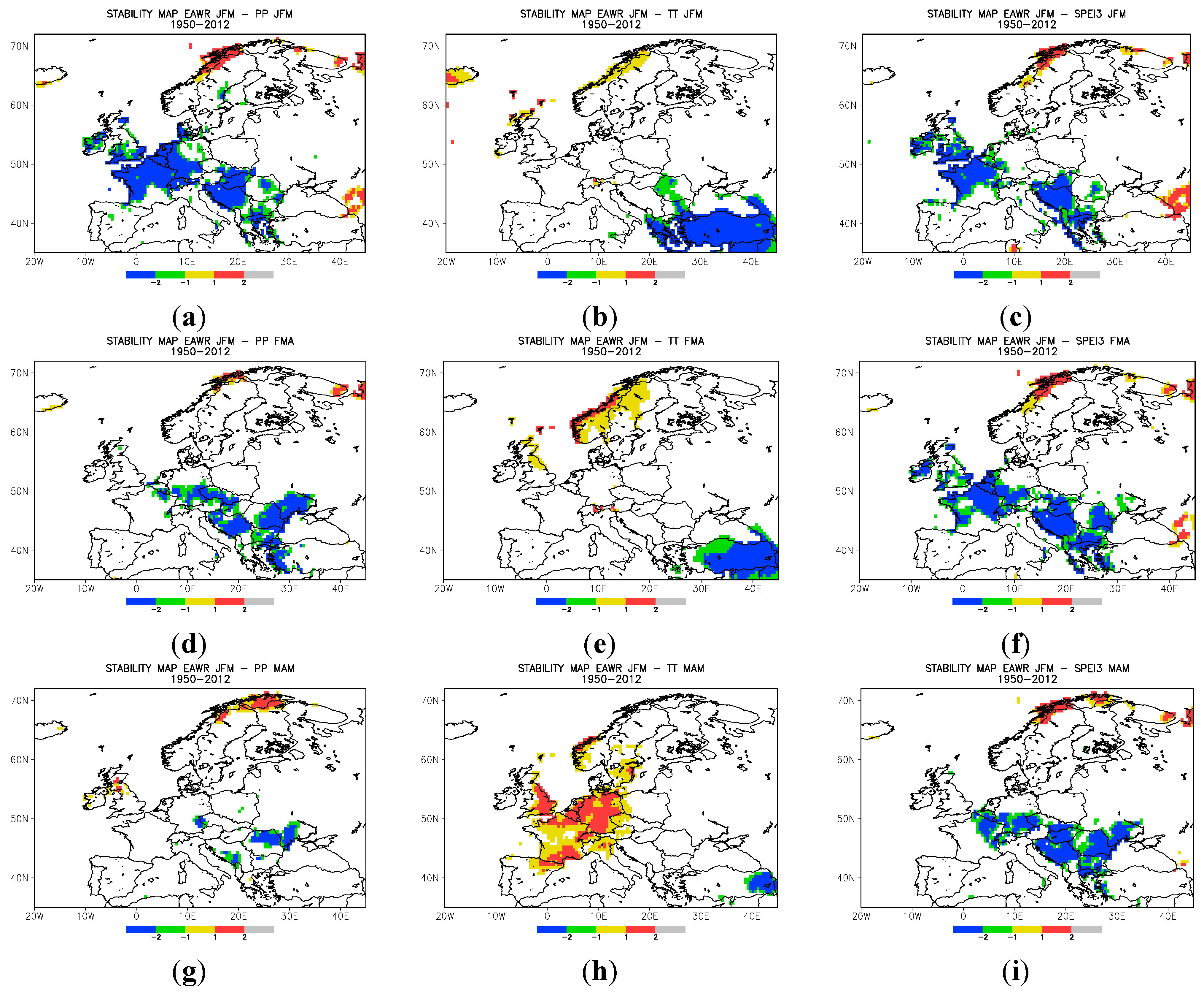
Figure 8 shows the stability maps between JFM EAWR and PP, TT and SPEI3, which are defined as regions where the running correlation in a 21-year window does not change the sign. The green (blue) and yellow (red) regions coincide with the regions where the correlation between JFM EAWR and the PP field is statistically significant at 80% (90%) level. The stability map between JFM EAWR and JFM PP (Figure 8a) shows small stable regions over the western part of Europe and Balkans. During early spring (Figure 8d) these regions extend all over the southern part of Europe (negative correlations) and the north-western part of the Scandinavian Peninsula (positive correlations), while in late spring (Figure 8g) there is no EAWR signal in the precipitation variability, except some small regions (e.g., northern part of Romania).

Figure 8. Stability maps of the correlation between JFM EAWR and Precipitation (first column), Temperature (second column) and SPEI3 (third column) for (a–c) January to March; (d–f) February to April and (g–i) March to May. Regions where the correlation is stable, positive, and significant at the 90% (80%) level for at least 80% of the windows are shaded red (yellow). The corresponding regions where the correlation is stable but negative are shaded blue (green).

Figure 8. Stability maps of the correlation between JFM EAWR and Precipitation (first column), Temperature (second column) and SPEI3 (third column) for (a–c) January to March; (d–f) February to April and (g–i) March to May. Regions where the correlation is stable, positive, and significant at the 90% (80%) level for at least 80% of the windows are shaded red (yellow). The corresponding regions where the correlation is stable but negative are shaded blue (green).

For mid-winter the stability map between JFM EAWR and JFM TT (Figure 8b) shows stable regions just over Bulgaria (negative stable correlation). By mid-spring the negative stable regions remain almost the same (Figure 8e), but significant positive correlations appear over the Scandinavian Peninsula. EAWR influence persists by late-spring especially over the central part of Europe (positive stable correlations), while over the Balkans the influence of EAWR almost disappears (Figure 8h).

In the case of SPEI3 the stability maps show persistent stable regions, from late winter to late spring (Figure 8c,f,i) over the central and the eastern part of Europe. The stable regions identified for PP, TT and SPEI3 can give a potential predictive skill based on the JFM EAWR index for the upcoming hydroclimate in late spring over Europe.

4. Conclusions

In summary, this study has investigated the relationship between the EAWR teleconnection pattern and the hydroclimatology of the European region from mid-winter to early spring. The research presented here contributes to a better understanding of how interannual phenomenon influences the climate over the European region. The influence of a prominent European teleconnections pattern over the whole European region, namely EAWR, which has a strong impact over the climate variability on the southeastern part of Europe and the Mediterranean region [27,28], has received little attention from the scientific community. The positive phase of EAWR leads to cold air advection from the north towards the southern part of Europe and eastern Mediterranean region [9].

According to [8] EAWR is characterized by significant decadal variations and trends which were related to the variability of the Eastern Mediterranean rainfall. Although there is not enough evidence to show if the trend observed in the EAWR pattern is subject to the influence of climate change or if the future climate will be characterized by a positive EAWR regime, our results show that at least a part of the variability in the climate of Europe can be linked to this mode of variability.

Despite the fact that EAWR has previously been linked to precipitation anomalies over the Mediterranean region [9,27] and with cyclonic activity, storminess and wind events over the same region [11], no actual study exists which takes into account the influence of mid-winter EAWR on the early to late spring precipitation, temperature and drought variability over Europe. The purpose of this paper was to identify a link between mid-winter EAWR and spring precipitation and temperature for the whole European region.

It is shown that prior to mid-winter there is little EAWR signature in the 500 hPa geopotential height anomalies. The classical EAWR pattern starts to develop in mid-winter and persist until late spring. The positive phase of EAWR in mid-winter is typically associated with drier than normal conditions over the southern part of Europe and wetter than normal conditions over the Scandinavian Peninsula. This pattern persists until early spring, while during the late spring no significant relationship between mid-winter EAWR and PP exists.

The EAWR signal was found to be more pronounced in the temperature field in late spring. Positive EAWR phase in mid-winter is associated with warmer than normal conditions over most of the central and northern part of Europe and colder than normal conditions over the southern part of Europe. This link between mid-winter EAWR and TT persists until late spring.

Concluding, the main findings of this study are: (1) EAWR has a strong impact on the coupling between the sub-tropical Atlantic Jet and the African Jet, which in turn affects the climate variability over Europe; (2) the strongest impact of the mid-winter EAWR over the European precipitation is in mid-winter and early spring over the Scandinavian Peninsula and the central and eastern part of Europe; (3) the link between mid-winter EAWR and European temperature persists from mid-winter to late spring, giving the possibility of a potential predictive skill for the spring temperature and (4) the link between mid-winter EAWR and European PP, TT and SPEI3 has found to be stable in time. By identifying the effects of the EAWR on the European hydroclimatology could help us to improve our knowledge in order to better understand and predict the interannual variations in precipitation and temperature.

References

1. Wallace, J.M.; Gutzler, D.S. Teleconnections in the geopotential height field during the Northern Hemisphere winter. Mon. Weather Rev. 1981, 109, 784–812. [Google Scholar]
2. Barnston, A.G.; Livezey, R.E. Classification, seasonality and persistence of low frequency atmospheric circulation patterns. Mon. Weather Rev. 1987, 115, 1083–1126. [Google Scholar]
3. Hurrell, J.W. The North Atlantic Oscillation: Climatic Significance and Environmental Effect; American Geophysical Union: Washington, DC, USA, 2003; EOS 84, No. 8. [Google Scholar]
4. Quadrelli, R.; Wallace, J.M. A simplified linear framework for interpreting patterns of Northern Hemisphere wintertime climate variability. J. Clim. 2004, 17, 3728–3744. [Google Scholar] [CrossRef]
5. Trenberth, K.E.; Hurrell, J.W.; Stepaniak, D.P. The Asian monsoon: Global perspectives. In Asian Monsoon; Wang, B., Ed.; Praxis Publishing Ltd.: Las Vegas, NV, USA, 2005; pp. 67–87. [Google Scholar]
6. Hurrell, J.W.; Deser, C. North Atlantic climate variability: The role of the North Atlantic Oscillation. J. Mar. Syst. 2009, 78, 28–41. [Google Scholar] [CrossRef]
7. Hurrell, J.W. Decadal trends in the North Atlantic oscillation: Regional temperatures and precipitation. Science 1995, 269, 676–679. [Google Scholar] [CrossRef]
8. Krichak, S.O.; Kishcha, P.; Alpert, P. Decadal trends of main Eurasian oscillations and the Mediterranean precipitation. Theor. Appl. Climatol. 2002, 72, 209–220. [Google Scholar] [CrossRef]
9. Krichak, S.O.; Alpert, P. Decadal trends in the East Atlantic–West Russia pattern and Mediterranean precipitation. Int. J. Climatol. 2005, 25, 183–192. [Google Scholar] [CrossRef]
10. Rimbu, N.; Onac, B.P.; Racovita, G. Large-scale anomaly patterns associated to temperature variability inside Scarisoara Ice Cave. Int. J. Climatol. 2012, 32, 1495–1502. [Google Scholar] [CrossRef]
11. Nissen, K.M.; Leckebusch, G.C.; Pinto, J.G.; Renggli, D.; Ulbrich, S.; Ulbrich, U. Cyclones causing wind storms in the Mediterranean: Characteristics, trends and links to large-scale patterns. Nat. Hazards Earth Syst. Sci. 2010, 10, 1379–1391. [Google Scholar] [CrossRef]
12. Climate Prediction Center:. Available online: http://www.cpc.ncep.noaa.gov/data/teledoc/eawruss.shtml.
13. Torrence, C.; Compo, G.P. A practical guide to wavelet analysis. Bull. Am. Meteorol. Soc. 1998, 79, 61–78. [Google Scholar] [CrossRef]
14. Harris, I.; Jones, P.D.; Osborn, T.J.; Lister, D.H. Updated high-resolution grids of monthly climatic observations. Int. J. Climatol. 2013. [Google Scholar] [CrossRef]
15. Vicente-Serrano, S.M.; Beguería, S.; López-Moreno, J.I. A multi-scalar drought index sensitive to global warming: The Standardized Precipitation Evapotranspiration Index—SPEI. J. Clim. 2010, 23, 1696–1718. [Google Scholar] [CrossRef]
16. McKee, T.B.N.; Doesken, J.; Kleist, J. The relationship of drought frequency and duration to time scales. In Proceedings of the Eight Conference on Applied Climatology, Anaheim, CA, USA, 17–22 January 1993; pp. 179–184.
17. Kalnay, E.; Kanamitsu, M.; Kistler, R.; Collins, W.; Deaven, D.; Gandin, L.; Iredell, M.; Saha, S.; White, G.; Woollen, J.; et al. The NMC/NCAR 40-year reanalysis project. Bull. Am. Meteorol. Soc. 1996, 77, 437–471. [Google Scholar] [CrossRef]
18. Peixoto, J.P.; Oort, A.H. Physics of Climate; Springer: New York, NY, USA, 1992; p. 520. [Google Scholar]
19. Von Storch, H.; Zwiers, F.W. Statistical Analysis in Climate Research; Cambridge University Press: Cambridge, UK, 1999; p. 494. [Google Scholar]
20. Lohmann, G.; Rimbu, N.; Dima, M. Where can the Arctic Oscillation be reconstructed? Towards a reconstruction of climate modes based on stable teleconnections. Clim. Past Discuss. 2005, 1, 17–56. [Google Scholar] [CrossRef]
21. Rimbu, N.; Dima, M.; Lohmann, G.; Musat, I. Seasonal prediction of Danube flow variability based on stable teleconnection with sea surface temperature. Geophys. Res. Lett. 2005. [Google Scholar] [CrossRef]
22. Ionita, M.; Lohmann, G.; Rimbu, N. Prediction of Elbe discharge based on stable teleconnections with winter global temperature and precipitation. J. Clim. 2008, 21, 6215–6226. [Google Scholar] [CrossRef]
23. Hoskins, B.J.; Draghici, I.; Davies, H.C. A new look at the ω-equation. Q. J. R. Meteorol. Soc. 1978, 104, 31–38. [Google Scholar]
24. Rimbu, N.; Lohmann, G.; Felis, T.; Pätzold, J. Shift in ENSO teleconnections recorded by a northern Red Sea coral. J. Clim. 2003, 16, 1414–1422. [Google Scholar] [CrossRef]
25. Deser, C. On the teleconnectivity of the “Arctic Oscillation”. Geophys. Res. Lett. 2000, 27, 779–782. [Google Scholar] [CrossRef]
26. Knippertz, P.; Ulbrich, U.; Marques, F.; Corte-Real, J. Decadal changes in the link between El Niño and spring North Atlantic oscillation and European-North African rainfall. Int. J. Climatol. 2003, 23, 1293–1311. [Google Scholar] [CrossRef]
27. Krichak, S.O.; Tsidulko, M.; Alpert, P. Monthly synoptic patterns associated with wet/dry conditions in the eastern Mediterranean. Theor. Appl. Climatol. 2000, 65, 215–229. [Google Scholar] [CrossRef]
28. Ziv, B.; Dayan, U.; Kushnir, Y.; Roth, C.; Enzel, Y. Regional and global atmospheric patterns governing rainfall in the southern Levant. Int. J. Climatol. 2006, 26, 55–73. [Google Scholar] [CrossRef]