Trends and Spatial Patterns of Drought Affected Area in Southern South America

Abstract

Based on 56 rainfall stations, which cover the period 1961–2008, we analyzed the presence of trends in the drought-affected area over southern South America (SSA) at different time scales. In order to define drought conditions, we used the standardized precipitation index, which was calculated on time scales of 1, 3, 6, 9 and 12 months. The trends were estimated following both a linear and a non-linear approach. The non-linear approach was based on the residual of the empirical mode decomposition, a recently proposed methodology, which is robust in presence of non-stationary data. This assessment indicates the existence of reversals in the trends of the drought affected, area around the 1990s, from decreasing trends during the first period to increasing trends during the recent period. This is indicative of the existence of a low-frequency variability that modulates regional precipitation patterns at different temporal scales, and warns about possible future consequences in the social and economic sectors if trends towards an increase in the drought affected area continue.

1. Introduction

Drought is perceived as one of the costliest and less understood natural disasters, given the difficulties to define its beginning and end, its slow development, and its multiple regional features. Therefore, it is important to investigate the temporal and spatial characteristics of droughts to provide a framework for sustainable water resources management, especially in semi-arid regions [1]. In these regions, desertification processes can interact with the occurrence of drought events, with significant impact on the environment and the population. Therefore, the identification of the role of droughts within the physical and social backgrounds could provide a better comprehension regarding improving the response and mitigation of its impacts. In the case of Southern South America (SSA), droughts are a recurrent phenomenon, with impacts evident in the reduction of crop yields, streamflow deficiencies, and consequent problems for hydropower generation.

The analysis of the temporal and spatial patterns of droughts contributes, in a significant way, to the evaluation of the dynamics of climate in a particular region. The preparedness and planning for a drought depend on the information about its areal extent, severity, and duration [2]. On an operational assessment, the National Oceanic and Atmospheric Administration (NOAA) continuously monitors the percentage of dry area over the United States and its impacts on agricultural and hydrological systems [3]. In SSA, the main meteorological centers of the region (SMN in Argentina and CPTEC in Brazil) analyze the spatial evolution of droughts on multiple time scales. The knowledge of the percentage of meteorological stations with drought conditions can be useful for the quantification of the spatial extension of the drought events [4]. In this way, Krepper and Zucarelli [5] defined as critical dry months those in which 30% of the study area is affected by precipitation values below one standard deviation from the mean. The authors found a relationship between the amount of critical months and the time scale considered for the definition of dry and wet periods over the La Plata Basin. Another relevant research was carried out by Barrucand et al. [6], who considered, as a drought index, the percentage of locations with precipitation lower than the median within a given region. They considered that a month is dry if at least 80% of the meteorological stations of the region recorded a precipitation value lower than the median, and analyzed its associated monthly circulation patterns.

During the second half of the 20th century, linear trends in precipitation over SSA showed a significant increase at different time scales [7,8,9,10]. Taking into account the non-linear character of climate variations, it is necessary to evaluate methodologies that allow a correct quantification of this kind of temporal variations. Such studies were carried out by Minetti et al. [11] and Rivera et al. [12], who analyzed the non-lineal trends in the annual total amounts of precipitation and in the annual number of dry days, respectively, through a cubic polynomial fit. Another relevant study was carried out by Krepper and Zucarelli [5], who applied singular spectrum analysis to the standardized precipitation index time series in the La Plata Basin, for the identification of non-linear trends. This methodology was also applied by Bordi et al. [13] for the estimation of non-linear trends in dryness and wetness over Europe. Other studies that analyzed the evolution of a drought affected area have been performed over Portugal [14] and Italy [15]; while a linear trend assessment of the rainfall shortages was carried out by Di Lena et al. [16] over Central Italy, Lana et al. [17] over Northeast Spain, and Lloyd-Hughes and Saunders [18] over Europe. In addition to the current evaluation of recent trends, several studies evaluated the future evolution of drought affected areas, based on global climate models and multiple scenarios. A global assessment of the projected changes can be found in Sheffield and Wood [19], who found substantial increases in the spatial extent of drought during the 21st century for most regions of the world.

It is expected that this non-linear signal, present in the precipitation temporal patterns, can be found in other variables, such as the spatial extension of drought events, although its behavior could be different over time and deserves a proper investigation. This paper addresses some aspects related to the spatial and temporal variability of the percentage of locations with drought conditions in SSA. For that purpose, we used the standardized precipitation index (SPI) in time scales of 1 (SPI1), 3 (SPI3), 6 (SPI6), 9 (SPI9), and 12 (SPI12) months, and for three levels of severity: moderate, severe, and extreme drought. This allows the representation of dry conditions that affect both the agricultural and hydrological sectors and, therefore, the economy of the regions considered.

2. Data and Methodology

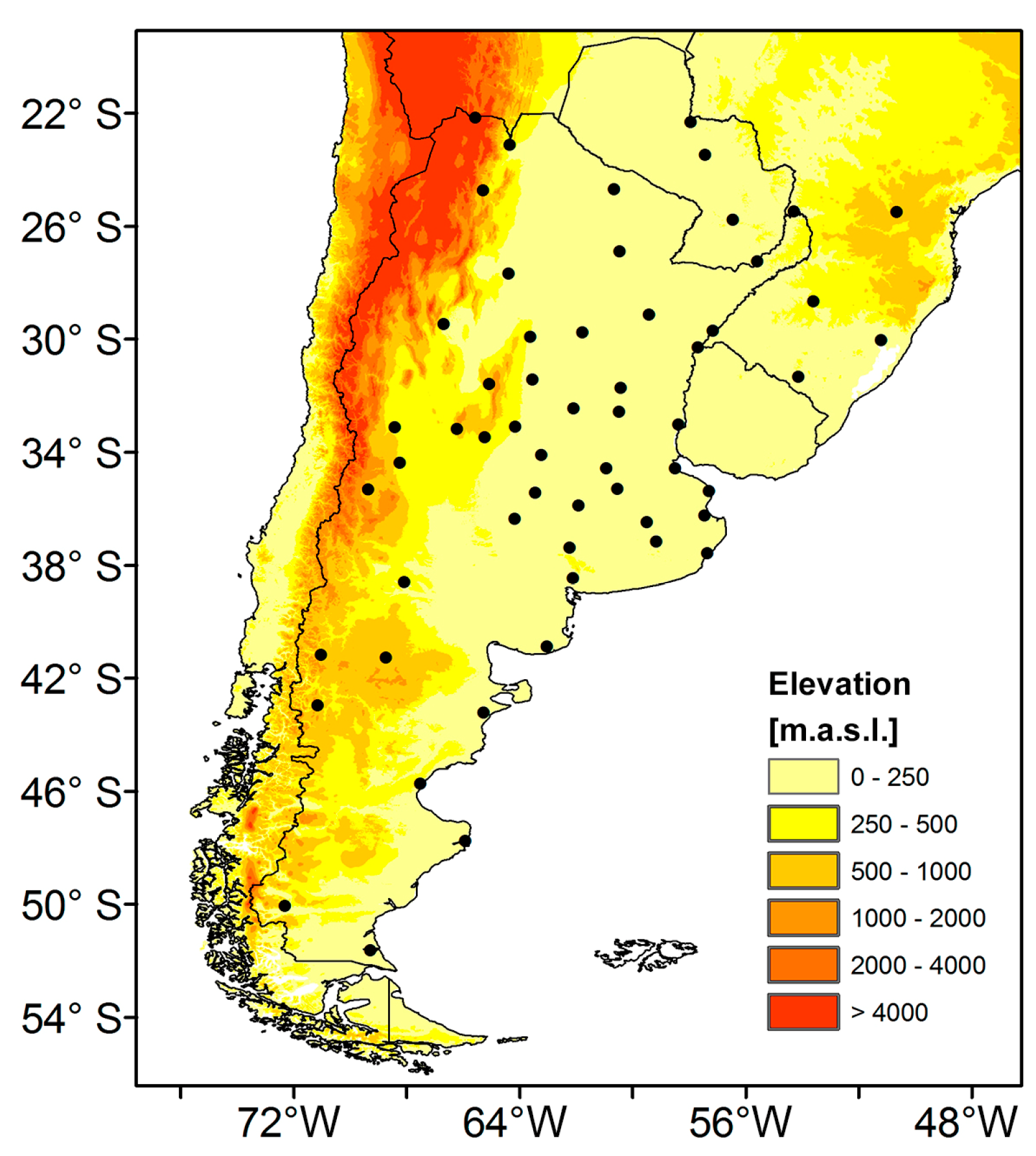
2.1. Precipitation Data

Precipitation is the main factor that controls the development and persistence of meteorological drought conditions [18]. Therefore, it is the variable considered for the analysis and recognition of this kind of drought. The database for the study consists of 56 monthly precipitation time series that cover the period 1961–2008, located in the portion of South America, south of 20°S, which are part of the CLARIS LPB database [20]. The distribution of the meteorological stations is shown in Figure 1. Quality control procedures are detailed in [20] and we also included a homogeneity control using the Standard Normal Homogeneity Test [21], the Pettit test [22], and the Buishand test [23]. These three additional tests identified inhomogeneities in 4 of the 56 precipitation time series, which correspond to climatic jumps and not to instrumental factors, given the spatial distribution of the dates of the changes (not shown). Therefore, no corrections were applied to the precipitation time series.

2.2. Standardized Precipitation Index

The standardized precipitation index (SPI) was developed by McKee et al. [24] with the purpose of drought definition and monitoring. During the last decade, this index became one of the most popular drought indicators, being valuable for its theoretical aspects, its robustness, and versatility for drought analysis [25]. The SPI has also been recommended by the Lincoln Declaration on Drought Indices [26] and according to Rivera and Penalba [27] is the most adequate drought index for SSA. Conceptually, the SPI represents the number of standard deviations from which a given precipitation value is above or below the long-term climatological average in a particular location. The SPI is a powerful, flexible index that is simple to calculate and is widely used in the region by the main agencies of weather (National Weather Services of Argentina, Brazil, Chile, Paraguay and Uruguay), agriculture (Brazilian Agricultural Research Corporation, Argentinean Center of Survey and Evaluation of Agricultural and Natural Resources), and water resources (General Directorate of Water Resources of Chile). A detailed description of the calculation of the SPI can be found in Lloyd-Hughes and Saunders [18].

Figure 1. Spatial distribution of the meteorological stations used in the study.

Figure 1. Spatial distribution of the meteorological stations used in the study.

In this work, we analyzed time scales of 1, 3, 6, 9, and 12 months, which were widely used in the literature [28]. Following Penalba and Rivera [29], a drought event was defined as the period of time where SPI values are below to −1.0. The percentage of meteorological stations with SPI values corresponding to moderate, severe, and extreme drought conditions can be used to quantify the spatial extension of drought events. Therefore, for each month of the 1961–2008 period, we calculated the percentage of locations with drought conditions. Three levels of severity were considered for the analysis of the drought affected area: moderate, severe, and extreme drought conditions. Table 1 indicates the thresholds for the SPI values for each category, with its probability of occurrence. Hence, we obtained three time series of drought affected area for each of the five time scales, which correspond to the different drought severity levels. In all the cases, the time series of the drought affected area in the moderate category include locations with severe and extreme drought, and the time series in the severe category include locations with extreme drought.

Table 1. SPI categories.

Category	SPI	Probability
Wet (W)	≥1.00	15.9%
Normal (N)	−0.99 to 0.99	68.2%
Moderate drought (MD)	−1.49 to −1.00	9.2%
Severe drought (SD)	−1.99 to −1.50	4.4%
Extreme drought (ED)	≤−2.00	2.3%

Table 1. SPI categories.

Category	SPI	Probability
Wet (W)	≥1.00	15.9%
Normal (N)	−0.99 to 0.99	68.2%
Moderate drought (MD)	−1.49 to −1.00	9.2%
Severe drought (SD)	−1.99 to −1.50	4.4%
Extreme drought (ED)	≤−2.00	2.3%

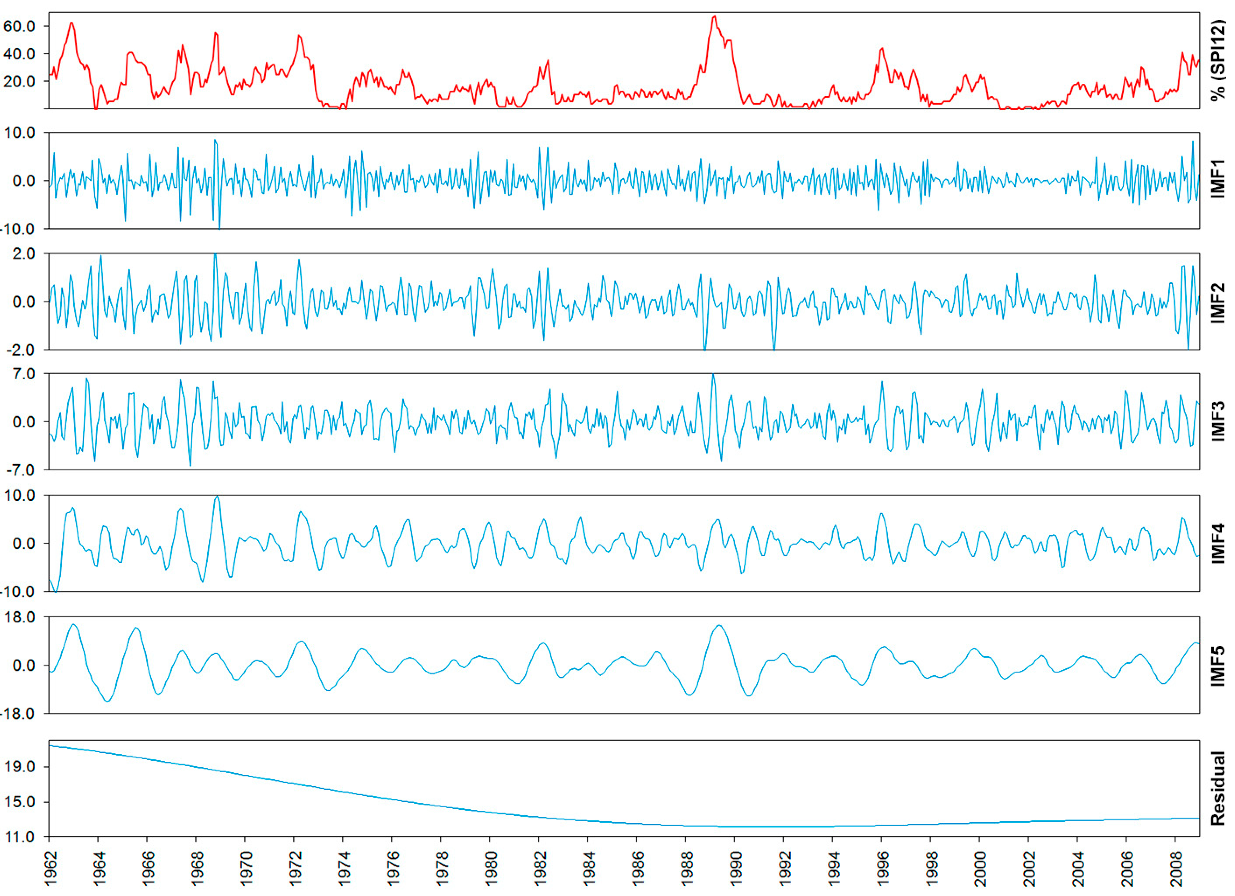
2.3. Trends Estimation

The linear trends were calculated for the period 1961–2008. A straight line was adjusted to each time series by using the linear regression method of least squares. The adjustment was evaluated by the correlation coefficient of Pearson, r, which reflects the degree of linear dependency between two datasets. The significance of the coefficients was evaluated on the confidence level of 95%.

For the estimation of the non-linearity present in the time series of the percentage of locations with drought conditions, we used the empirical mode decomposition (EMD) [30]. This method decomposes a time series in a finite number of components, called intrinsic mode functions (IMF), and a residual trend. The residual of the composition corresponds to the non-linear trend estimation. This method is robust in the presence of non-stationary data and is adequate for the study of time series, which possesses non-linear variations [31]. According to Sang et al. [32], EMD can be an effective alternative for trend identification in hydrological time series. The detailed algorithm of the EMD is described in [30,33]. The basics of the calculation are described as follows:

• Initialize: i = 1, and define r₀ = x(t).
• Identify the extremes (maximum and minimum) of r₀, and generate the upper and lower envelopes connecting all the local extrema through a cubic spline interpolation.
• Calculate the mean envelope m_{(j = 1)}.
• Subtract the mean envelope to the time series in order to obtain the first sub time series h_{(j = 1)} (h_{(j = 1)} = r₀ − m_{(j = 1)}).
• Treat h_{(j = 1)} as r₀ and repeat steps 2 to 4 with j = j + 1 as many times as needed, until the envelopes being symmetric to zero mean under certain criteria. The final h_(j) is designated as C_i.
• Define again r₀ = x(t) − C_i and i = i + 1, and then repeat steps 2 to 5. When i = N and the residual becomes a monotonic function or a function only containing one internal extremum from which no more IFM can be extracted, a complete sifting process of series x(t) by EMD stops. The decomposition results can be expressed as:

  $$x\left(t\right)={\displaystyle \sum }_{i=1}^N{C}_i+R_N$$

  (1)

where N is the number of IMFs separated from series x(t), and C_i is the ith IMF.

We considered a version of EMD that was improved by Huang et al. [33] taking into account the presence of mode mixing and based upon an ensemble of the decomposition with adaptive noise [34]. Its main advantages in comparison with the original EMD are discussed by Colominas et al. [35]. As an example, Figure 2 shows the results of the EMD from the time series of a drought affected area based on SPI12. Only the first 5 IMF are shown, from a total of 9 IMF, which together with the residual are enough to represent the original signal. The EDM firstly extracted the higher frequency variations from the data, represented by the IMF1, and the successive applications of the algorithm produced the remaining IMFs. Low frequency variations are represented by the higher-order IMFs, and the residual represents the non-linear trend of the data.

Figure 2. Empirical mode decomposition of the drought affected area based on the SPI12. Only the first five intrinsic mode functions are shown. The top panel shows the original signal (in red), while the lower panel shows the residual of the decomposition.

Figure 2. Empirical mode decomposition of the drought affected area based on the SPI12. Only the first five intrinsic mode functions are shown. The top panel shows the original signal (in red), while the lower panel shows the residual of the decomposition.

The use of this methodology for the analysis of non-linear trends in SSA is novel and will be applied in this research to the time series of drought affected area. Several studies applied the EMD for the identification of the main modes of variability and the assessment of non-linear trends in variables like precipitation and temperature [36] and indices like the Southern Oscillation Index and the Indian Ocean Dipole Index [37]. Assitionally, the EMD potential for climatological indices forecasting was assessed by Iyengar et al. [38] and Karthikeyan and Kumar [39].

3. Results and Discussion

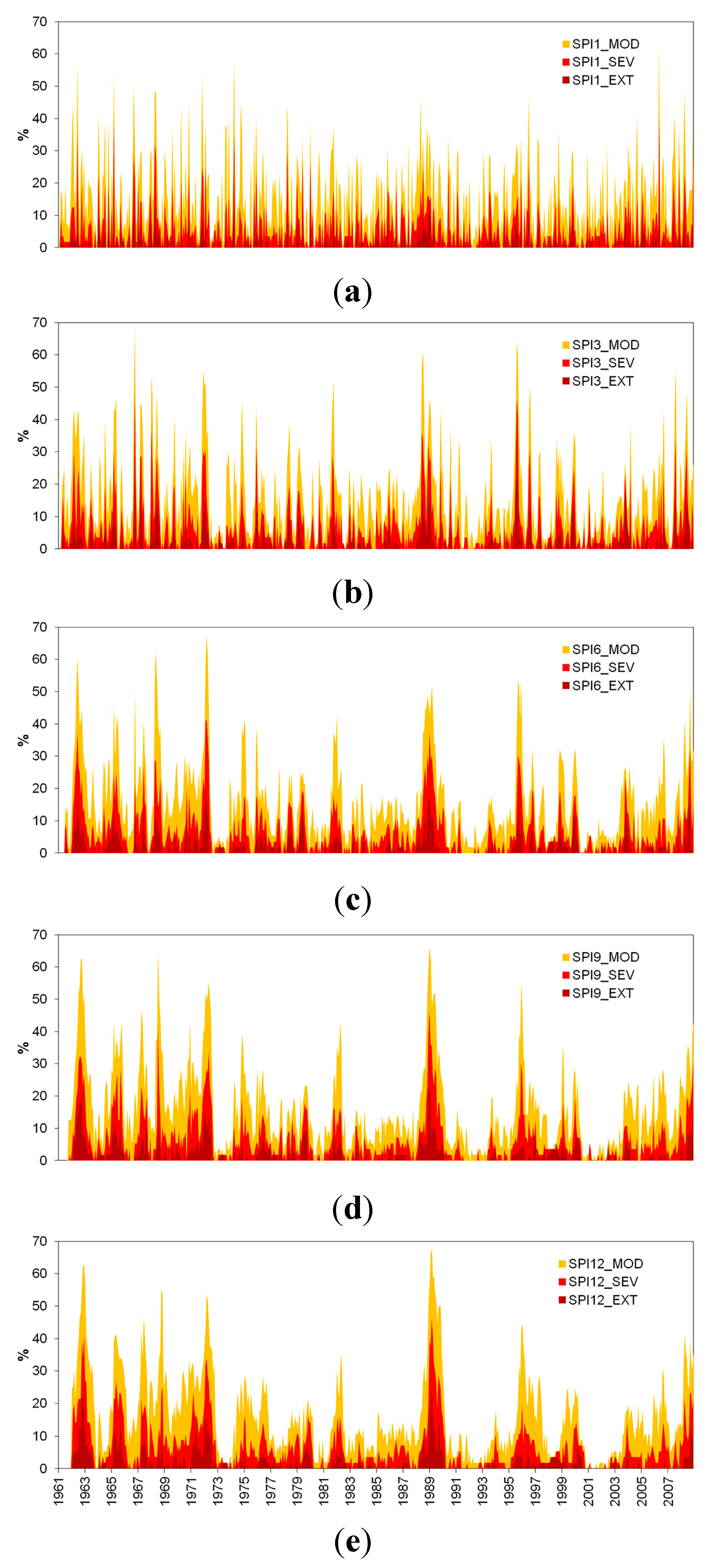
3.1. Temporal Evolution of the Number of Meteorological Stations with Drought Conditions

From a vulnerability point of view, the situations when a great portion of the study area is under drought conditions must be considered. Figure 3 shows the temporal evolution of the percentage of stations with moderate (SPI ≤ −1.0), severe (SPI ≤ −1.5), and extreme (SPI ≤ −2.0) drought conditions for the five temporal scales calculated in the SSA. For the three severity levels, the high frequency temporal variability in the time series decreases as the time scale for the calculation of SPI increases. In the case of SPI1 a strong temporal irregularity is observed, alternating periods of dryness and wetness (Figure 3a). During the years 1962, 1965, 1966, 1971, 1974, and 2006, more than 50% of the stations were affected with moderate drought conditions. This indicates that most of the drought events that affected a great portion of SSA were recorded during the 1960s and 1970s, although prolonged periods of drought were recorded during 1988–1989 and 1995–1996. In the case of SPI3, during the years 1966, 1988, and 1995, more than 60% of the stations were affected by moderate drought conditions (Figure 3b). Moreover, during the 1995 event, more than 45% of the stations presented severe drought conditions, and were located mainly in the central-east and north-east portions of Argentina. As the time scale increases, the major drought events affecting large portions of SSA are better defined. This is verified for the time scales of 6, 9, and 12 months (Figure 3c–e, respectively). The drought affected area based on the SPI6 shows that the events of 1962, 1968, and 1972 affected more than 60% of the analyzed stations (Figure 3c). During the 1972 drought, more than 40% of the locations presented severe drought conditions. The percentages of stations identified through SPI9 show greater values between 1961 and 1972, where the 1962 and 1968 events stand out. In this time scale, the drought event recorded between 1988 and 1989 was one of the most important of the 1961–2008 period, covering more than 60% of the analyzed stations (Figure 3d). Finally, if we consider the precipitation deficits in a 12-month time scale, the events of 1962 and 1988–1989 stand out, which affected more than 60% of the study area (Figure 3e). From that percentage, 20% corresponds to extreme drought conditions. Through this analysis stands the practicality of SPI12 to capture multi-annual drought events and decadal variations in the percentage of locations with drought conditions. It was notable that the increase in the drought affected area, since 2001, reached 40% of the study area during 2008 in all the time scales.

Table 2 shows the maximum percentage of locations with drought for each time scale and severity level, with the corresponding month and year of occurrence. In the case of moderate droughts, in all cases, more than 60% of SSA was affected by drought during certain periods of time, which depends upon the time scale considered. These extreme events were particularly damaging, given that rainfed agriculture represents 92% of the agricultural areas in Argentina, 90% in Bolivia and Brazil, 97% in Uruguay, and 60% in Paraguay [40]. The drought of 1988–1989 affected a higher number of locations in time scales of nine and 12 months. In the case of the time scale of six months, the drought of 1971–1972 showed the higher percentages of drought affected areas. The drought event of 1965–1966 affected the highest percentage of locations in the time scale of three months, which indicates that, from the agricultural point of view, this event was one of the most damaging of the 1961–2008 period. These results indicate that droughts are a phenomenon of limited extension, in which diverse local and regional factors interact to determine their extreme values, given the heterogeneous pattern observed in SSA in the five temporal scales analyzed.

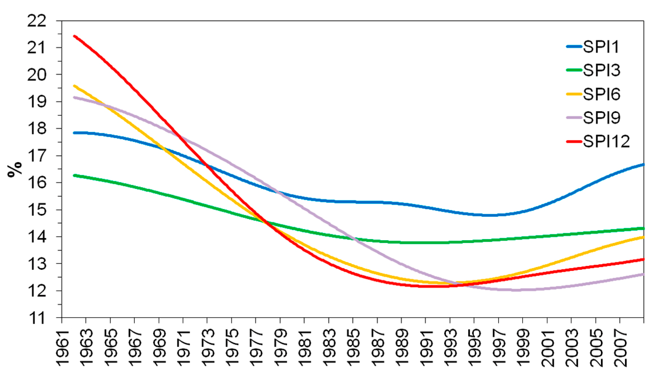
3.2. Trends in the Number of Meteorological Stations with Moderate Drought Conditions

A linear trend estimation was performed to assess the long-term changes in the evolution of the drought affected area for every severity level and time scale considered. Significant decreases were observed for the time scales of six, nine, and 12 months in all the severity levels. In the case of the temporal evolution based on the SPI6, the percentage of locations with moderate drought shows a significant negative linear trend that represents approximately a decrease of 1.8% per decade. The SPI9 time series shows a significant negative linear trend of approximately 2.4% per decade for the moderate level. For the time scale of 12 months, the time series of the percentage of locations with moderate drought conditions shows a significant decrease of 2.8% every 10 years, while this change decreases to 1.5% for the severe category. The percentage of change per decade for the three severity levels indicates that as the time scale increases, the area affected by drought decreases further.

Figure 3. Temporal evolution of the percentage of meteorological stations with drought conditions during 1961–2008. Orange, vermillion, and red colors indicate moderate, severe, and extreme conditions, respectively. (a) SPI1; (b) SPI3; (c) SPI6; (d) SPI9; (e) SPI12.

Figure 3. Temporal evolution of the percentage of meteorological stations with drought conditions during 1961–2008. Orange, vermillion, and red colors indicate moderate, severe, and extreme conditions, respectively. (a) SPI1; (b) SPI3; (c) SPI6; (d) SPI9; (e) SPI12.

Table 2. Maximum percentage of locations with drought conditions for each temporal scale and severity level, together with the date of occurrence.

Category	Moderate		Severe		Extreme
Time Scale	Max %	Date	Max %	Date	Max %	Date
1	62.50	May 2006	41.07	May 2006	23.21	March 1965
3	67.86	October 1966	48.21	October 1966	26.79	October 1966
6	67.86	March 1972	41.07	February and March 1972	17.86	February 1972
9	66.07	January 1989	46.43	January 1989	23.21	January 1989
12	67.86	March 1989	46.43	March 1989	25.00	March 1989

Table 2. Maximum percentage of locations with drought conditions for each temporal scale and severity level, together with the date of occurrence.

Category	Moderate		Severe		Extreme
Time Scale	Max %	Date	Max %	Date	Max %	Date
1	62.50	May 2006	41.07	May 2006	23.21	March 1965
3	67.86	October 1966	48.21	October 1966	26.79	October 1966
6	67.86	March 1972	41.07	February and March 1972	17.86	February 1972
9	66.07	January 1989	46.43	January 1989	23.21	January 1989
12	67.86	March 1989	46.43	March 1989	25.00	March 1989

Based on Figure 3, an increase in the drought affected area over the last decade in all the time scales considered was observed. Given the non-linearity of precipitation variations in SSA over the last century, we assessed the low frequency variations in the moderate drought affected area through the residual of the EMD. To better assess these temporal variations, we decided to analyze only the evolution of moderate drought conditions given the continuity of the time series (i.e., lack of long periods with zero values). Figure 4 shows the residuals of the EMD of the percentage of locations with moderate drought for the five time scales considered. While all the trends show a decrease in the percentage of stations affected by moderate drought, a reversion is verified between the end of the 1980s and mid-1990s. The years of the reversion are dependent upon the time scale considered; for example, for time scales of six and 12 months, the change is evident during the first half of the 1990s, while for time scales of one and nine months, this is evident during the second half of the same decade. These results were observed in other variables by Krepper and Zucarelli [5] and Rivera et al. [12], and warn about the existence of a low frequency variability that can lead to an increase in drought affected area during the beginning of the 21st century. The residual of the EMD for the SPI12 time series accounts for almost 15% of the total variance, while this percentage contributes to almost 10% for the SPI9 variability and 8% for SPI6. Recent trends in the drought affected area for the moderate severity level were calculated for the 1999–2008 period as the percentage of change. In all the time scales a significant positive trend was observed, with the higher magnitudes observed at time scales of one and six months. Table 3 summarizes the main findings of this section.

Figure 4. Non-linear trends estimation through the residual of the EMD of the time series of percentage of stations with moderate drought conditions for the period 1961–2008 in the five time scales considered.

Figure 4. Non-linear trends estimation through the residual of the EMD of the time series of percentage of stations with moderate drought conditions for the period 1961–2008 in the five time scales considered.

Table 3. Year of the trend reversal in the evolution of the drought affected area for the five scales considered, percentage of change (slope) every 10 years, based in the period 1961–2008 and recent trends (percentage of change) for the 1999–2008 period. Significant values are in bold.

Category	Moderate			Severe	Extreme
Time Scale	Year of Trend Reversal	Slope/10 Years	Recent Trend	Slope/10 Years	Slope/10 Years
1	1996	−0.38	3.40	−0.21	−0.11
3	1990	−0.96	0.65	−0.43	−0.10
6	1991	−1.78	2.44	−0.98	−0.35
9	1998	−2.38	1.09	−1.18	−0.56
12	1991	−2.81	1.11	−1.49	−0.70

Table 3. Year of the trend reversal in the evolution of the drought affected area for the five scales considered, percentage of change (slope) every 10 years, based in the period 1961–2008 and recent trends (percentage of change) for the 1999–2008 period. Significant values are in bold.

Category	Moderate			Severe	Extreme
Time Scale	Year of Trend Reversal	Slope/10 Years	Recent Trend	Slope/10 Years	Slope/10 Years
1	1996	−0.38	3.40	−0.21	−0.11
3	1990	−0.96	0.65	−0.43	−0.10
6	1991	−1.78	2.44	−0.98	−0.35
9	1998	−2.38	1.09	−1.18	−0.56
12	1991	−2.81	1.11	−1.49	−0.70

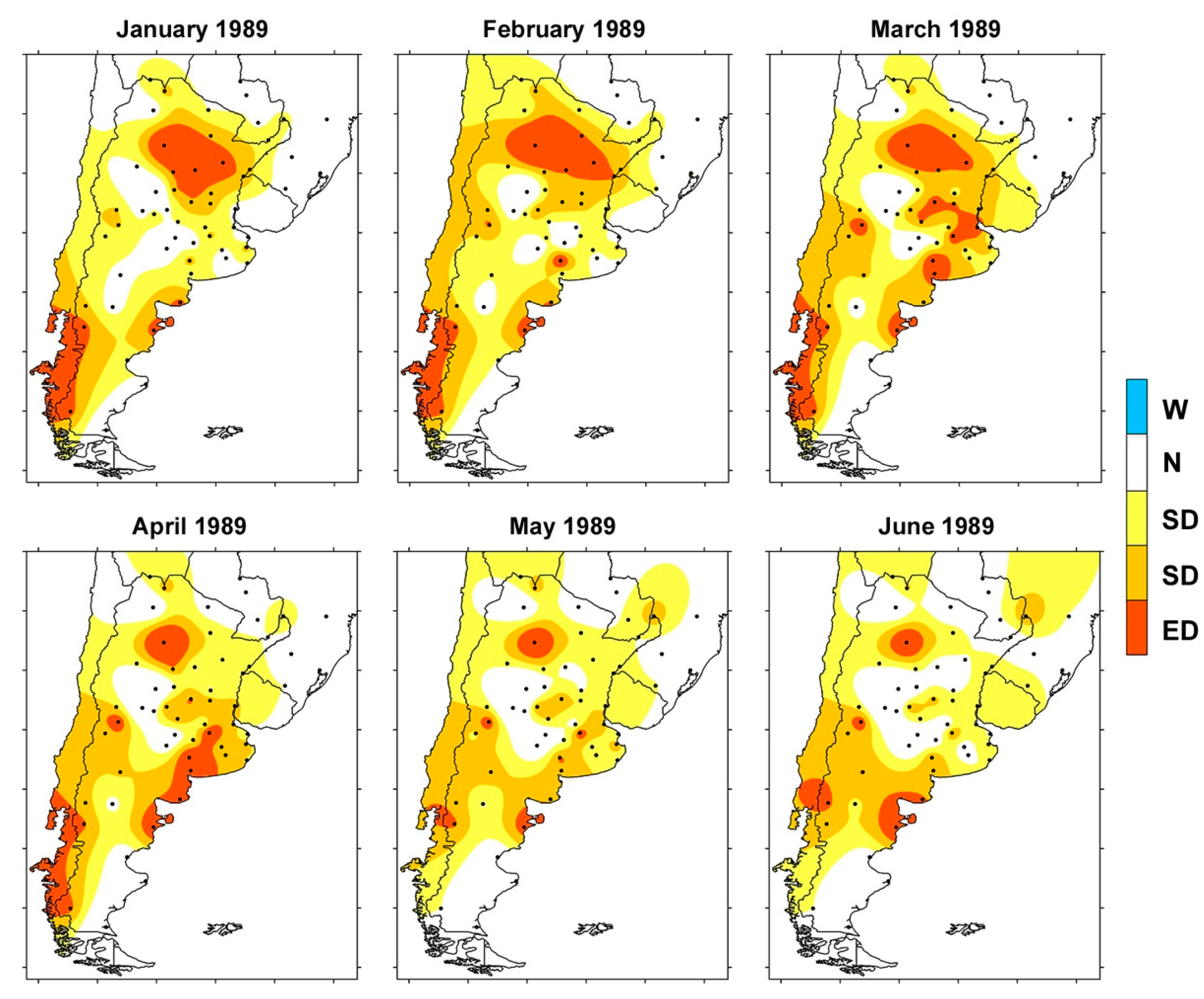
3.3. Spatial Evolution of Major Droughts over SSA

Based on the results presented in Table 2, it is worthwhile to discuss the spatial evolution of the main drought events over SSA. Both the spatial extent and evolution of major droughts present several differences between events, given that the atmospheric patterns can affect several regions in different ways. For example, the drought of 1971–1972 affected a great percentage of locations particularly on time scale of six months (Table 2). This event mainly affected the central-western portion of SSA, a semi-arid region that strongly depends on water to sustain the regional economies [41], and the central portion of the La Plata Basin. Another relevant drought event was recorded for the time scale of three months during the spring of 1966, a season which is determinant for agricultural production. This event affected particularly the humid Pampas and the north-western Patagonia regions. The drought conditions began during September over the lower portion of the La Plata Basin and progressed south during October, with extreme drought conditions over most of the Pampas region (not shown). This drought event affected the highest number of locations in comparison with other drought events and time scales (Table 2) and had a relatively short duration, which warns about the random spatial and temporal behavior of short-term droughts.

One of the most damaging drought events was recorded during 1988–1989. This particular event had its greatest extension on time scales of nine and 12 months (Table 2), affecting the central portion of the study area and the northern portion of Patagonia. Figure 5 shows the temporal evolution of the drought affected area during the months of January to June, 1989, for SPI12. Persistent drought conditions affected the central and eastern regions of Argentina. Taking into account the drought severity levels, this event progressed toward the Pampas region during the months of March and April, reaching the category of severe drought. An increase in the drought severity levels over northern Patagonia is evident, being the main region affected by drought during the month of June, 1989. This event had significant impacts in the economic sector, with losses of 20% of the total volume of grain [42] and the minimum levels of hydroelectric power generation over the Comahue region, located in north-western Patagonia.

Figure 5. Temporal evolution of the 1988–1989 drought during the months of January to June 1989 for the SPI12 time series. Drought categories are indicated in Table 1.

Figure 5. Temporal evolution of the 1988–1989 drought during the months of January to June 1989 for the SPI12 time series. Drought categories are indicated in Table 1.

In the three drought events (1966, 1971–1972 and 1988–1989) a negative anomaly in the sea surface temperature over the El Niño 3.4 region was observed (i.e., La Niña conditions). Significant decreases in corn productivity documented by Minetti et al. [43] were also related to La Niña years, especially during the 1988–1989 event. Other sub-seasonal factors, such as the development of blocking conditions over the Southern Pacific Ocean [44], can contribute with the onset and intensification of drought events over SSA.

4. Conclusions

In this work we analyzed the temporal evolution of the drought affected area in Southern South America during the 1961–2008 period, for time scales ranging from one to 12 months. The presence of non-linear trends in these time series was identified through a recently proposed method, based on the residual of the empirical mode decomposition. Even though the linear trends indicate that the percentage of locations with drought conditions is diminishing, which is related to the increase of precipitation over the study area observed during the second half of the 20th century, the non-linear trends analysis showed that the time series presented a reversion during the decade of the 1990s. Due to the significant impact of these trends in the agricultural production and the hydroelectric generation, its continuous monitoring and interpretation is necessary. This should be performed through methodologies, as those used in this research, which are robust in the presence of non-stationary data. This non-linearity in the drought affected area is indicative of a low-frequency climatic oscillation that modulates the regional aspects of precipitation in SSA. According to Junquas et al. [45], trends in summer precipitation over SSA will decrease during the first half of the 21st century, which is in agreement with the trends found during recent years and warns about the severe consequences that these low-frequency oscillations can have at a regional level.

It was verified that droughts are a phenomenon of limited extension, in which several local factors act to determinate its extreme values, given the heterogeneous pattern observed in SSA. However, the analysis showed that the period of time from 1961 to 1972 was characterized by the occurrence of several widespread droughts in all the time scales. The most severe episodes affected a great portion of SSA, with the droughts of 1966 and 1988–1989 affecting with moderate drought conditions in more than 60% of the region, and more than 45% at a severe level.

References

1. Kim, T.W.; Valdés, J.B.; Aparicio, J. Frequency and spatial characteristics of droughts in the Conchos river basin, Mexico. Water Int. 2002, 27, 420–430. [Google Scholar] [CrossRef]
2. Mishra, A.K.; Singh, V.P. Drought modeling—A review. J. Hydrol. 2011, 403, 157–175. [Google Scholar] [CrossRef]
3. National Oceanic and Atmospheric Administration. State of the Climate. Available online: http://www.ncdc.noaa.gov/sotc/drought/ (accessed on 18 July 2014).
4. Skansi, M.M.; Veiga, H.; Garay, N.G.; Podestá, G. Períodos secos en la región noreste de Argentina descriptos con el índice de precipitación estandarizado. In Proceedings of the XI Argentine Congress of Meteorology (CONGREMET), Mendoza, Argentina, 28 May–1 June 2012.
5. Krepper, C.M.; Zucarelli, V. Climatology of water excess and shortages in the La Plata Basin. Theor. Appl. Climatol. 2012, 102, 13–27. [Google Scholar] [CrossRef]
6. Barrucand, M.G.; Vargas, W.M.; Rusticucci, M.M. Dry conditions over Argentina and the related monthly circulation patterns. Meteorol. Atmos. Phys. 2007, 98, 99–114. [Google Scholar] [CrossRef]
7. Castañeda, M.; Barros, V. Las tendencias de la precipitación en el cono sur de América al este de los Andes. Meteorológica 1994, 19, 23–32. [Google Scholar]
8. Penalba, O.C.; Vargas, W.M. Interdecadal and interannual variations of annual and extreme precipitation over Central-Northeastern Argentina. Int. J. Climatol. 2004, 24, 1565–1580. [Google Scholar] [CrossRef]
9. Barros, V.R.; Doyle, M.E.; Camilloni, I.A. Precipitation trends in southeastern South America: relationship with ENSO phases and with low-level circulation. Theor. Appl. Climatol. 2008, 93, 19–33. [Google Scholar] [CrossRef]
10. Penalba, O.C.; Robledo, F.A. Spatial and temporal variability of the frequency of extreme daily rainfall regime in the La Plata Basin during the 20th century. Clim. Chang. 2010, 98, 531–550. [Google Scholar] [CrossRef]
11. Minetti, J.L.; Vargas, W.M.; Poblete, A.G.; Acuña, L.R.; Casagrande, G. Non-linear trends and low frequency oscillations in annual precipitation over Argentina and Chile, 1931–1999. Atmósfera 1931, 16, 119–135. [Google Scholar]
12. Rivera, J.A.; Penalba, O.C.; Bettolli, M.L. Inter-annual and inter-decadal variability of dry days in Argentina. Int. J. Climatol. 2013, 33, 834–842. [Google Scholar] [CrossRef]
13. Bordi, I.; Fraedrich, K.; Sutera, A. Observed drought and wetness trends in Europe: An update. Hydrol. Earth Syst. Sci. 2009, 13, 1519–1530. [Google Scholar] [CrossRef]
14. Santos, J.F.; Pulido-Calvo, I.; Portela, M.M. Spatial and temporal variability of droughts in Portugal. Water Resour. Res. 2010. [Google Scholar] [CrossRef]
15. Rossi, G.; Bonaccorso, B.; Nicolosi, V.; Cancelliere, A. Characterizing drought risk in a Sicilian river basin. In Coping with Drought Risk in Agriculture and Water Supply Systems; Iglesias, A., Garrote, L., Cancelliere, A., Cubillo, F., Wilhite, D., Eds.; Springer: Berlin, Germany, 2009; pp. 187–219. [Google Scholar]
16. Di Lena, B.; Vergni, L.; Antenucci, F.; Todisco, F.; Mannocchi, F. Analysis of drought in the region of Abruzzo (Central Italy) by the Standardized Precipitation Index. Theor. Appl. Climatol. 2014, 115, 41–52. [Google Scholar] [CrossRef]
17. Lana, X.; Serra, C.; Burgueño, A. Patterns of monthly rainfall shortage and excess in terms of the standardized precipitation index for Catalonia (NE Spain). Int. J. Climatol. 2001, 21, 1669–1691. [Google Scholar] [CrossRef]
18. Lloyd-Hughes, B.; Saunders, M.A. A drought climatology for Europe. Int. J. Climatol. 2002, 22, 1571–1592. [Google Scholar] [CrossRef]
19. Sheffield, J.; Wood, E.F. Projected changes in drought occurrence under future global warming from multi-model, multi-scenario, IPCC AR4 simulations. Clim. Dyn. 2008, 31, 79–105. [Google Scholar] [CrossRef]
20. Penalba, O.C.; Rivera, J.A.; Pántano, V.C. The CLARIS LPB database: Constructing a long-term daily hydro-meteorological dataset for La Plata Basin, Southern South America. Geosci. Data J. 2014, 1, 20–29. [Google Scholar] [CrossRef]
21. Alexandersson, H. A homogeneity test applied to precipitation data. J. Climatol. 1986, 6, 661–675. [Google Scholar] [CrossRef]
22. Pettit, A.N. A non-parametric approach to the change-point detection. Appl. Stat. 1979, 28, 126–135. [Google Scholar] [CrossRef]
23. Buishand, T.A. Some methods for testing the homogeneity of rainfall records. J. Hydrol. 1982, 58, 11–27. [Google Scholar] [CrossRef]
24. McKee, T.B.; Doesken, N.J.; Kleist, J. The relationship of drought frequency and duration to time scales. In Proceedings of the Eight Conference on Applied Climatology, Anaheim, CA, USA, 17–23 January 1993; American Meteorological Society: Boston, MA; USA, 1993; pp. 179–184. [Google Scholar]
25. Vicente-Serrano, S.M.; Lopez-Moreno, J.I. The influence of atmospheric circulation at different spatial scales on winter drought variability through a semi-arid climatic gradient in northeast Spain. Int. J. Climatol. 2006, 26, 1427–1453. [Google Scholar] [CrossRef]
26. Hayes, M.; Svoboda, M.; Wall, N.; Widhalm, M. The Lincoln Declaration on drought indices: Universal meteorological drought index recommended. Bull. Am. Meteorol. Soc. 2011, 92, 485–488. [Google Scholar] [CrossRef]
27. Rivera, J.A.; Penalba, O.C. Comparison of the performance of five indices for drought characterization in La Plata Basin. Perspectives towards a multi-scale monitoring system. In Proceedings of the 2011 WCRP Open Science Conference, Denver, CO, USA, 23–27 October 2011.
28. Wu, H.; Hayes, M.J.; Weiss, A.; Hu, Q. An evaluation of the standardized precipitation index, the China-Z index and the statistical Z-score. Int. J. Climatol. 2001, 21, 745–758. [Google Scholar] [CrossRef]
29. Penalba, O.C.; Rivera, J.A. Future changes in drought characteristics over Southern South America projected by a CMIP5 multi-model ensemble. Am. J. Clim. Chang. 2013, 2, 173–182. [Google Scholar] [CrossRef]
30. Huang, N.E.; Shen, Z.; Long, R.; Wu, M.C.; Shih, E.H.; Zheng, Q.; Tung, C.C.; Liu, H.H. The empirical mode decomposition method and the Hilbert spectrum for non-linear and non-stationary time series analysis. Proc. R. Soc. Lond. Ser. A Math. Phys. Eng. Sci. 1998, 454, 903–995. [Google Scholar] [CrossRef]
31. Wu, Z.; Huang, N.E. Ensemble empirical mode decomposition: A noise-assisted data analysis method. Adv. Adapt. Data Anal. 2009, 1, 1–41. [Google Scholar] [CrossRef]
32. Sang, Y.F.; Wang, Z.; Liu, C. Comparison of the MK test and EMD method for trend identification in hydrological time series. J. Hydrol. 2014, 510, 293–298. [Google Scholar] [CrossRef]
33. Huang, N.E.; Shen, Z.; Long, S.R. A new view of nonlinear water waves: The Hilbert spectrum. Annu. Rev. Fluid Mech. 1999, 31, 417–457. [Google Scholar] [CrossRef]
34. Torres, M.E.; Colominas, M.A.; Schlotthauer, G.; Flandrin, P. A complete ensemble empirical mode decomposition with adaptive noise. In Proceedings of the 2011 IEEE International Conference on Acoustics, Speech and Signal Processing (ICASSP), Prague, Czech, 22–27 May 2011; pp. 4144–4147.
35. Colominas, M.A.; Schlotthauer, G.; Torres, M.E.; Flandrin, P. Noise-assisted EMD methods in action. Adv. Adapt. Data Anal. 2012. [Google Scholar] [CrossRef]
36. Srikanthan, R.; Peel, M.C.; McMahon, T.A.; Karoly, D.J. Ensemble empirical mode decomposition of Australian monthly rainfall and temperature data. In Proceedings of the 19th International Congress on Modelling and Simulation, Pert, WA, Australia, 12–16 December 2011; pp. 3643–3649.
37. Peel, M.C.; Srikanthan, T.A.; McMahon, T.A.; Karoly, D.J. Ensemble empirical mode decomposition of monthly climatic indices relevant to Australian hydrolicmatology. In Proceedings of the 19th International Congress on Modelling and Simulation, Pert, WA, Australia, 12–16 December 2011; pp. 3615–3621.
38. Iyengar, R.N.; Raghu Kanth, S.T.G. Intrinsic mode functions and a strategy for forecasting Indian monsoon rainfall. Meteorol. Atmos. Phys. 2005, 90, 17–36. [Google Scholar] [CrossRef]
39. Karthikeyan, L.; Kumar, D.N. Predictability of nonstationary time series using wavelet and EMD based ARMA models. J. Hydrol. 2013, 502, 103–119. [Google Scholar] [CrossRef]
40. Popescu, I.; Brandimarte, L.; Perera, M.S.U.; Peviani, M. Assessing residual hydropower potential of the La Plata Basin accounting for future user demands. Hydrol. Earth Syst. Sci. 2012, 16, 2813–2823. [Google Scholar] [CrossRef]
41. Compagnucci, R.H.; Agosta, E.A.; Vargas, W.M. Climatic change and quasi-oscillations in central-west Argentina summer precipitation: Main features and coherent behaviour with southern African region. Clim. Dyn. 2002, 18, 421–435. [Google Scholar] [CrossRef]
42. Kogan, F.N. Contribution of remote sensing to drought early warning. In Early Warning Systems for Drought Preparedness and Drought Management, Proceedings of 2000 An Expert Group Meeting in Early Warning Systems for Drought Preparedness and Drought Management, Lisboa, Portugal, 5–7 September 2000; Wilhite, D.A., Sivakumar, W., Wood, D.A., Eds.; World Meteorological Organization: Geneva, Switzerland, 2000; pp. 86–100. [Google Scholar]
43. Minetti, J.L.; Vargas, W.M.; Vega, B.; Costa, M.C. Las sequías en la pampa húmeda: Impacto en la productividad del maíz. Rev. Bras. Meteorol. 2007, 22, 218–232. [Google Scholar] [CrossRef]
44. Alessandro, A.P. Acciones bloqueantes alrededor de los setenta grados oeste en el sur de Sudamérica. Meteorológica 2005, 30, 3–25. [Google Scholar]
45. Junquas, C.; Vera, C.; Li, L.; le Treut, H. Summer precipitation variability over Southeastern South America in a global warming scenario. Clim. Dyn. 2012, 38, 1867–1883. [Google Scholar] [CrossRef]