Bayesian Nonparametric Measurement of Factor Betas and Clustering with Application to Hedge Fund Returns

Abstract

We define a dynamic and self-adjusting mixture of Gaussian Graphical Models to cluster financial returns, and provide a new method for extraction of nonparametric estimates of dynamic alphas (excess return) and betas (to a choice set of explanatory factors) in a multivariate setting. This approach, as well as the outputs, has a dynamic, nonstationary and nonparametric form, which circumvents the problem of model risk and parametric assumptions that the Kalman filter and other widely used approaches rely on. The by-product of clusters, used for shrinkage and information borrowing, can be of use to determine relationships around specific events. This approach exhibits a smaller Root Mean Squared Error than traditionally used benchmarks in financial settings, which we illustrate through simulation. As an illustration, we use hedge fund index data, and find that our estimated alphas are, on average, 0.13% per month higher (1.6% per year) than alphas estimated through Ordinary Least Squares. The approach exhibits fast adaptation to abrupt changes in the parameters, as seen in our estimated alphas and betas, which exhibit high volatility, especially in periods which can be identified as times of stressful market events, a reflection of the dynamic positioning of hedge fund portfolio managers.

1. Introduction

We use a novel dynamic and arbitrary mixture of Gaussian Graphical Models (GGM) to describe sets of returns with complex relationships in a dynamic, nonstationary and nonparametric form and, at the same time, extract new nonparametric, nonstationary and dynamic alphas (excess returns) and betas (exposures to risk factors) of those returns. The procedure we follow builds on the formal mathematical model devised by [1]. However, we adjust their approach to financial settings, by constructing an approach that will extract and construct implied nonparametric alphas and betas, which are key parameters of interest in financial applications. A simulation study will offer an initial insight to the level of outperformance of our approach against some traditionally used approaches. Additionally, we apply this procedure to hedge fund index data for the period January 1994 to June 2009, and find that our estimated alphas or excess returns are, on average, 0.75% per month. These alphas are 0.13% per month higher than those estimated applying OLS for the same period and, thus, our procedure uncovers that average hedge fund alphas could be underestimated when measured using OLS.

Our paper contributes to the existing literature mainly in two ways: first, it devises a new methodology to extract market dynamic alphas and betas, which is less bound to widely-extended assumptions on the parametric structure of returns. This approach is especially beneficial when the generating process is very dynamic with varying numbers of clusters (and series within clusters). Second, we provide information about clusters that can be used by allocators/decision-makers outside of the more traditional expected return/risk-reward settings (for example, through relation-in-distress measurements, which could allow allocators to reduce exposures in combinations of assets/funds that tend to cluster when volatilities rise or when returns drop, or increase exposures in combinations that tend to de-cluster when returns drop, increasing the level of expected “idiosyncracy-under-stress” when it’s most needed in the portfolio). Our approach allows for the joint modelling of multiple series both as dependent and independent sets of variables. Our methodology finds a natural application in problems where a set of variables is driven by another set of variables in a difficult-to-parametrize, non-stationary fashion.

Our application, hedge fund returns, can be seen as jointly driven by a set of factors, as opposed to fixed asset benchmarks, with exposures to those varying over time. Our results show much higher alphas to those considered through more traditional methods, indicating sufficiently relevant differences to consider this approach as one of non-marginal impact. These contrast with the alphas outlined in recent literature (see Titman and Tiu [2], Mamaysky et al. [3], Ferson and Schadt [4], Patton and Ramadorai [5], for a recent review). Furthermore, our estimated alphas and betas exhibit very high volatility, particularly in periods which can be identified as times of stressful market events. This is in line with the existence of many dynamic drivers in this particular application, such as dynamic market conditions, dynamic internal fund allocations, shift in portfolio manager styles and exposures, as well as dynamics of liquidity parameters of the individual funds. These findings question the constant alpha and beta assumption implicit in some studies conducted to measure hedge fund performance, as well as in the dynamic (yet parametric) approaches presented in others like [3]. Ours is more in line with a dynamic mixture model, with the mixtures viewed as the flexible, accomodating distributions to the different approaches to portfolio management and exposures of funds over time.

The question of investment performance measurement (in both absolute and relative terms) has received increasing attention by both academicians and practitioners. The hedge fund industry, the focus of our application, has grown rapidly during the past two decades, and institutional investors such as endowments and pension funds have gradually increased their allocations to hedge funds. According to Hedge Fund Research, the total number of funds around the world grew to around ten thousand and total assets under management (AUM) reached around 2 trillion US dollars by the end of 2013. The hedge fund industry was severely affected by the global financial crisis of 2008–2009, with the total number of funds and AUM dropping by around a third during the crisis, although they mostly recovered by the end of 2010. The analysis of their returns, however, is nontrivial as the underlying processes are both complex and dynamic. Hedge fund managers change their allocations, positions, and their styles over time. Risk or leverage limits are often imposed. Market events change the focus of specific managers and new managers come and go with different styles. Additionally, the alpha of different styles changes over time, with periods where some styles outperform/underperform others over arbitrary periods before they revert. Even within a hedge fund group/style, there will be much different approaches that will generate very different return series (for example, depending on the frequency at which they operate). As such, any modelling approach must be sufficiently flexible to account for these (and other) changes in the nature of the return process over time. We offer a flexible, nonstationary, nonparametric approach that borrows information across dynamic clusters, but, more importantly, makes neither parametric assumptions on the nature of the (dynamic) alphas and betas nor on their autocorrelation structure. This approach, although we focus on the Hedge Fund return application, is applicable to any set of return series where the dynamics are too complex and unknown to be modelled using parametric assumptions, yet a dynamic model is needed for all the key elements of the series (alphas, betas and clusters).

It is important to mention that the focus of this paper is mainly descriptive, rather than inferential. Due to the high variability and the dynamic nature of the series we model, and the cluster dependence on the drivers of the series, although inference is technically possible, our focus is on providing a better understanding of the returns. A more accurate understanding of alphas, betas and clustering styles will provide decision-makers with new sources of information. This information, although usable directly in the allocation process (through the alphas and betas), finds also a natural space indirectly through cluster analysis (for example, putting limits on combined weights assigned to series that have a high probability of clustering in distress periods).

The measurement of alpha, in the case hedge funds returns, as well as other complex return series, is complicated by their dynamic use of strategies that include long and short positions, as well as derivatives that result in very dynamic factor exposures against fixed benchmarks. This in turn generates non-linear returns that require tailored benchmarks. Furthermore, and according to [6], risk exposures of hedge funds have also declined in response to the rising dominance of institutional investors replacing family offices and private individuals as the primary source of investor capital. These same authors argue that the rapid growth of hedge funds has been responsible for the decline in their performance between the 1990s and mid-2000s and that perhaps “all the low-hanging fruits have been picked.” This view questions the use of a constant, mean-reverting level for the alphas, and calls for non-stationary models for key paramers, such as the one proposed in this paper. Additionally, it is also questionable that betas to key factors can be stationary, especially as funds deploy new ways to exploit competitive advantages (for example, as funds/sectors move to trading in higher frequencies, betas of those funds to factors defined in lower frequencies may diminish).

When empirically tested, many of the approaches assume that the coefficients of the regressions are constant over time (or come from a constant distribution). If, in fact, these coefficients are time-varying and non-stationary, then the estimated parameters using these models would be unreliable. In the context of our application, as an example, [7] propose to measure the conditional performance of hedge fund indices using a stochastic discount factor approach, which imposes fewer limitations on the behavior of underlying returns. They find that estimated alphas, which are found to be positive, are similar when hedge fund performance is measured assuming either of the following four cases: (i) an absolute return approach (e.g., Alpha = $R_i-R_f$); (ii) a single-factor, fixed-exposure approach (e.g., CAPM); (iii) a single-factor, linear time-varying exposure approach (e.g., Merton’s model); and (iv) an extension of Merton’s approach consisting of a multi-factor, linear time-varying exposure approach. This finding of similar estimated alphas regardless of the model used leads them to conclude that better models are needed to measure hedge fund performance. Our approach finds very different (across funds and over time) alphas and betas, which seems more in line with expectations of highly dynamic funds.

In a related prior approach, for a similar application, [3] address the issue of time variation in mutual fund factor loadings and develop a Kalman filter model to test for market-timing ability; showing that even though the Kalman filter model does not appear to exhibit market-timing ability at the daily frequency, it does so at the monthly frequency. While we focus our application on monthly returns, the flexibility of the design accomodates via a non-parametric approach to estimate dependence between alphas, making it less reliant on a strong parametric link between them over time, like the one imposed by the Kalman filter. Although a special case of our model and with another application in mind, [8] use a regime-switching beta model to measure dynamic risk exposures of hedge funds to various risk factors during different market volatility conditions. For interesting overlaps of our work with networks and graphical models please see [9,10].

Kosowski et al. [11] use Bayesian measures to estimate hedge fund alpha at the individual hedge fund level. These measures are based on the robust boostrap approach suggested by [12], and the Bayesian framework of [13]. They argue, in the same vein as [14,15,16], that hedge fund performance measures do not follow parametric normal distributions because these funds hold derivatives such as options, because of the dynamic nature of their trading strategies, and also due to small sample problems. These features of hedge fund performance help explain their finding that Bayesian nonparametric measures yield superior performance predictability relative to alphas estimated when specific parametric models are assumed.

The Bayesian paradigm provides in the case aforementioned, as well as ours, a natural, flexible tool to the fast estimation of the quantities of interest. Our approach is especially amenable for cases where small sample sizes also hinder many alternative approaches due to the (random) large dimensionality of the problem. The implementation of a Bayesian approach for measuring hedge fund performance should not be surprising, because Bayesian measures have been traditionally used to help overcome the small-sample problem typical of hedge fund returns1, making this also an area where our approach may become amenable.

Using a robust boostrap procedure, [11] also find that hedge fund performance at the top cannot be explained solely by luck, that performance persists at annual horizons, and that OLS alphas of top hedge funds tend to be incorrectly estimated. It is worth noticing that the model used in [11] is not only parametric in nature, and therefore exposed to model risk, but also stationary. On the contrary, the alphas, as well as the betas derived in our paper, are nonstationary and dynamic. To the best of our knowledge there is no previous work that employs a formal mathematical model to describe in a dynamic, nonstationary and nonparametric way multivariate returns against multivariate factors, and extract at the same time some new nonparametric, nonstationary and dynamic alphas and betas, under a clustering scheme for shrinking, and in a fully Bayesian approach.

Gaussian graphical models (GGMs), also called covariance selection models [22], are popular tools for modeling dependence across observables. GGMs assume that the returns generated by different asset classes and/or investment vehicles follow a joint multivariate Gaussian distribution, and explore the pattern of partial correlations to understand how the different outcomes influence each other. Because observations are assumed to follow a (arbitrary mixture of) multivariate Gaussian distribution, absence of partial correlation corresponds to a zero in the appropriate entry of the precision (inverse covariance) matrix and indicates that the variables are conditionally independent. The conditional independence patterns inferred in this way can be represented using a graph where nodes correspond to variables and an edge is present between two variables if they are conditionally dependent, and absent otherwise.

GGMs are a natural alternative to endogenous factor models as described in [23,24], which explain the joint multivariate outcome as a linear combination of a small number of unknown factors determined directly from the data being modeled2. However, GGMs are particularly appealing over these endogenous factor models because they allow researchers to asses conditional rather than marginal independence, which in turn makes it straightforward to distinguish between direct and indirect interactions between the variables. GGMs have been successfully applied in finance and econometrics (for example, see [1,28,29,30,31]), where they have been shown to provide interpretability and enhanced predictive performance. However, our extraction of cluster-implied alphas and betas adds a new layer of outputs to the existing literature, since they allow direct use of these parametric measures derived from a non-parametric setting.

The paper is organized as follows. Section 2 presents the statistical methods we employ. Section 3 offers sensitivity analysis and simulation exercises to compare our model to traditionally used models that pursue similar features of the data. In Section 4 we describe the data used in the study, and the application through hedge fund returns. Section 5 shows the main results obtained, while Section 6 offers the results of estimating time-varying alphas and betas, as well as cluster analysis, using the infinite hidden Markov model (iHMM-GGM) proposed by [1]. Finally, we outline our conclusions and potential extensions in Section 7.

2. Modeling Dependence among Asset Classes and Investment Vehicles

In this section we describe the statistical methodology. We will start by reviewing basic notions of Gaussian Graphical Models and their link with sparse (regularized) regression. Then, we will move to describe hidden Markov models that employ Gaussian Graphical Models to describe state-specific distributions.

2.1. Gaussian Graphical Models

Let ${\mathbf{z}}_t={(z_{1t},\dots ,z_{qt})}^{\prime }$ be a vector of observed returns, where $z_{it}$ represents the return of fund i over period t, for $t=1,\dots ,T$. A Gaussian graphical model for the sequence ${\mathbf{z}}_1,\dots ,{\mathbf{z}}_T$ assumes that observations are independent and identically distributed from a multivariate normal distribution, ${\mathbf{z}}_t\sim {\mathsf{N}}_q\left(\mu ,{\mathbf{K}}^{-1}\right)$, where μ is the vector of mean returns, G is a graph3 describing the conditional independence structure among the entries of ${\mathbf{z}}_t$, and $\mathbf{K}=\mathbf{K}\left(G\right)$ is a precision matrix such that ${\left[\mathbf{K}\left(G\right)\right]}_{i,j}=0$, if and only if the edge connecting node i and node j is missing from G.

Bayesian inference for GGMs proceeds by placing priors on the unknown parameters $(\mu ,\mathbf{K},G)$. A popular approach uses conjugate priors and factorizes the joint prior $p(\mu ,\mathbf{K},G)$ as

$$p(\mu ,\mathbf{K},G)=p\left(\mu \right|\mathbf{K}\left)p\right(\mathbf{K}\left|G\right)p\left(G\right)$$

where $p\left(\mu \right|\mathbf{K})$ is a multivariate Gaussian distribution $\mathsf{N}({\mu }_0,{(n_0\mathbf{K})}^{-1})$, $p\left(\mathbf{K}\right|G)$ corresponds to a G-Wishart prior [32], and $p\left(G\right)$ is a uniform distribution on the space of graphs. It is worthwhile to note that $\mathbf{K}$ is a function of the graph G since G will define the structure of zeroes $\mathbf{K}$ will have. This prior will model the parameters as independently as possible conditional on the graph G.

For small values of q, the posterior distribution of all model parameters can be computed in closed-form and inference is straightforward. For moderate to large values of q, the number of possible graphs is typically too large for explicit enumeration and Markov chain Monte Carlo algorithms that efficiently explore the space of graphs are typically required (for details and examples see [33,34,35], among others).

GGMs can be used for sparse regression [29]. Consider a standard multivariate regression model, which assumes that the conditional distribution of the response ${\mathbf{y}}_t$ given a vector of predictors ${\mathbf{x}}_t$ is Gaussian. In our manuscript ${\mathbf{y}}_t$ will be the cross-sectional vector of hedge fund returns at time t and ${\mathbf{x}}_t$ the vector of market risk factors. An equivalent model is implied by a joint Gaussian distribution on the vector ${\mathbf{z}}_t={({\mathbf{y}}_t^{\prime },{\mathbf{x}}_t^{\prime })}^{\prime }$. Indeed, if ${\mathbf{z}}_t\sim \mathsf{N}(\mu ,{\mathbf{K}}^{-1})$ where

$$\begin{array}{ccccc}\hfill \mu & =\left(\begin{array}{c}{\mu }^y\\ {\mu }^x\end{array}\right)\hfill & \hfill & \hfill \mathbf{K}& =\left(\begin{array}{cc}{\mathbf{K}}^{yy}& {\mathbf{K}}^{yx}\\ {\mathbf{K}}^{xy}& {\mathbf{K}}^{xx}\end{array}\right)\hfill \end{array}$$

then standard results for the multivariate Gaussian distribution imply that

$$\begin{array}{c}\hfill {\mathbf{y}}_t|{\mathbf{x}}_t\sim \mathsf{N}\left({\mu }^y-{\left({\mathbf{K}}^{yy}\right)}^{-1}{\mathbf{K}}^{yx}\left\{{\mathbf{x}}_t-{\mu }^x\right\},{\left({\mathbf{K}}^{yy}\right)}^{-1}\right)\end{array}$$

(1)

Estimates of this joint model can be used to construct estimates of the regression function. Indeed, if maximum likelihood methods are used to estimate μ and $\mathbf{K}$, then the estimates of the intercept and slopes from Equation (1) will be identical to those obtained through ordinary least squares (OLS). For example, in the Capital Asset Pricing Model (CAPM) the intercept α corresponds to ${\mu }^y+{\left({\mathbf{K}}^{xx}\right)}^{-1}{\mathbf{K}}^{xy}{\mu }^x$ while the market risk parameter β corresponds to $-{\left({\mathbf{K}}^{xx}\right)}^{-1}{\mathbf{K}}^{yx}$ [36]. On the other hand, placing a prior on $(\mu ,\mathbf{K})$ is equivalent to placing a prior distribution on the regression coefficients of a linear regression model together with a prior on the marginal distribution of ${\mathbf{x}}_t$. This procedure, although slightly more convoluted than simply placing a prior on the regression coefficients, can be easily generalizable to mixtures of Gaussian graphical models to generate nonparametric regression procedures.

We used the CAPM in the previous analysis because the CAPM is a linear model and the IHMM-GGM model that we are using is built as an approximation of infinite linear OLS models. Thus, we can compare our model to those models that are more commonly used in finance (linear models such as the CAPM and OLS multivariate regressions). Our approach is less constrained because it is nonparametric, dynamic and nonstationary, whereas the CAPM is parametric, nondynamic, and stationary.

2.2. Dynamic Mixtures of GGMs

Our discussion in the introduction suggests that hedge fund returns should not be assumed to be normally distributed, making the use of standard Gaussian graphical models potentially inappropriate for our application. To alleviate this issue we follow [1] and construct a hidden Markov model where the market fluctuates among an unknown number of clusters, and where hedge fund returns were generated from a collection cluster-specific GGMs. This structure for the hidden Markov model implies a nonparametric mixture model for the stationary (marginal) distribution on the market returns, which ensures that our model is capable of capturing all the stylized features of hedge fund returns that were discussed in Section 1.

More specifically, introduce cluster variables ${\xi }_1,\dots ,{\xi }_T$ with ${\xi }_t\in \{1,2,3,\dots \}$ and let

$$\begin{array}{cc}\hfill {\mathbf{z}}_t|{\mu }_{{\xi }_t},{\mathbf{K}}_{{\xi }_t},G_{{\xi }_t}& \sim \mathsf{N}\left({\mu }_{{\xi }_t},{\left\{{\mathbf{K}}_{{\xi }_t}\left(G_{{\xi }_t}\right)\right\}}^{-1}\right),\hfill \end{array}$$

i.e., conditional on the market being in cluster l (which corresponds to ${\xi }_t=l$), the observations are generated from a GGM with mean vector ${\mu }_l$ and precision matrix ${\mathbf{K}}_l$ such that its conditional independence structure is given by graph $G_l$. Therefore if $G_l$ has off-diagonal zeroes this corresponds to independence between specific asset returns. If we look at the analysis unconditional of ${\xi }_t$ then the same interpretation of independence does not carry through anymore.

To account for the sequential nature of the data we allow the cluster of the system to evolve as a Markov chain with a potentially infinite number of clusters,

$$\begin{array}{cc}\hfill \mathsf{Pr}({\xi }_t=l\mid {\xi }_{t-1}=k)& ={\pi }_{k,l}\hfill \end{array}$$

where the vector ${\mathit{\pi }}_k=({\pi }_{k,1},{\pi }_{k,2},{\pi }_{k,3},\dots )$ (containing the transition probabilities from cluster k to all other clusters) is given a Dirichlet process prior [37,38],

$$\begin{array}{cc}\hfill {\mathit{\pi }}_k|\alpha ,\mathit{\varpi }& \sim \mathsf{DP}(\alpha ,\mathit{\varpi }),\hfill \end{array}$$

independently for each k, where $\mathit{\varpi }=({\varpi }_1,{\varpi }_2,\dots )$ and

$$\begin{array}{cccc}\hfill {\varpi }_l& =v_l\prod _{k<l}\{1-v_k\},\hfill & \hfill v_l& \sim \mathsf{Beta}(1,\beta ).\hfill \end{array}$$

The Dirichlet process is an extension of the Dirichlet distribution to countably infinite spaces. Indeed, the model just described can be obtained as the limit of a finite hidden Markov model,

$$\begin{array}{cc}\hfill ({\pi }_{k,1},\dots ,{\pi }_{k,L})|\alpha ,\mathit{\varpi }& \sim \mathsf{Dirichlet}(\alpha {\varpi }_1,\dots ,\alpha {\varpi }_L)\hfill \\ \hfill ({\varpi }_1,\dots ,{\varpi }_L)\mid \beta & \sim \mathsf{Dirichlet}\left(\frac{\beta }{L},\dots ,\frac{\beta }{L}\right)\hfill \end{array}$$

as $L\to \infty$. Therefore, this specification implies that $\mathsf{E}\left({\mathit{\pi }}_k\right)=\mathit{\varpi }$, i.e., ϖ represent a common mean for the vector of transition probability across clusters, while α controls how much each ${\pi }_k$ deviates from this common mean.

The model we just described (called an infinite hidden Markov model, or iHMM, see [39,40]) admits a priori an unlimited number of clusters. However, the prior structure is such that a posteriori only a few distinct regimes are actually employed to fit the data. Hence, this infinite HMM (iHMM-GGM) allows us to automatically and parsimoniously estimate the number of clusters.

The iHMM specification above can be used to generate dynamic nonparametric estimates of the parameters of the CAPM. Indeed, conditioning on the cluster ${\xi }_t$ we can write an expression that is analogous to (1),

$$\begin{array}{c}\hfill {\mathbf{y}}_t|{\mathbf{x}}_t\sim \mathsf{N}\left({\mu }_{{\xi }_t}^y-{({\mathbf{K}}_{{\xi }_t}^{yy})}^{-1}{\mathbf{K}}_{{\xi }_t}^{yx}\left\{{\mathbf{x}}_t-{\mu }_{{\xi }_t}^x\right\},{({\mathbf{K}}_{{\xi }_t}^{yy})}^{-1}\right).\end{array}$$

In other words, the model clusters time periods according to the cluster to which they belong and assigns the same CAPM parameters to periods in the same cluster. Uncertainty on the cluster indicators ${\xi }_1,\dots ,{\xi }_T$ can be incorporated through model average, leading to flexible estimates.

Posterior computation for the iHMM involves the use of simulation-based Markov chain Monte Carlo algorithms. Given an initial guess for the model parameters, these iterative algorithms sequentially generate random realizations of blocks of parameters conditionally on the current values of the rest. After the algorithm has converged, these random draws can be used to produce approximate estimates of all parameters of interest, including point and interval estimates. For details, see [1]. The software we employed to fit our models is available from the authors by request.

Last but not least, finite mixture problems have been used in different scientific communities, such as unsupervised clustering in neural network applications, latent class analysis in the social sciences, and regime switching models in economics, among others [41]. A finite mixture model has a finite number of clusters or states and therefore is a special case of our iHMM-GGM, which has infinite. Moreover, setting two clusters for ${\xi }_t=1,2$ and noticing that our iHMM-GGM is also dynamic in nature, we get back a classical and well known regime switching model. For more on such conections between regime switching models and finite mixture models, please see [41] (Chapter 10).

3. Sensitivity Analysis and Simulation Exercises

3.1. Sensitivity

An important question to ask is whether the prior distribution on L (prior number of clusters) has any impact on its posterior distribution. The ideal scenario is when the posterior of L given the data does not change with different prior distributions of L, therefore making the estimation and algorithm robust to choices of prior. The prior on L implied by the Dirichlet process is given by [1]:

$$\begin{array}{c}\hfill p\left(L\right|{\alpha }_0,n)=S(n,L)n!{\alpha }_0^L\frac{\Gamma \left({\alpha }_0\right)}{\Gamma ({\alpha }_0+n)}\end{array}$$

(2)

where $S(n,L)$ denotes the Stirling number of the first kind [42]. We can conclude that the mean number of non-empty mixture components grows with ${\alpha }_0$, the concentration parameter the Dirichlet process $DP({\alpha }_0,M)$ which has a prior $\text{Gamma}(a,b)$ [1].

We tested the effect of the priors with a representative range of key parameters a and b. As detailed in Equation (2), the key parameters for the implied prior on L are the hyperparameters a and b. For these two hyperparameters, we define what could be a priori the boundaries of reasonable a priori values for the applications in this paper. Figure 1 includes the distribution of three of those priors that represent a reasonable range for the problem at hand:

• $\text{Gamma}(a=1,b=5)$. This is a strong, very informative, prior that maps into a distribution of the clusters with a prior mean of clusters = 2 and a standard deviation of the number of clusters = 2 (prior two moments included in each of the graphs in Figure 1). This would be appropriate if we believe that there is a very limited number of clusters in the data.
• $\text{Gamma}(a=1,b=1)$. This is a medium-intensity prior that implies a larger number of clusters on average, and a heavier tail. We chose this prior for our analysis due to the nature of our data, where we anticipated a large number of clusters, but were uncertain as to how many.
• $\text{Gamma}(a=5,b=5)$. This is a low-intensity, more vague, prior that implies a much larger number of clusters.

Figure 2 includes the posterior distribution of the number of clusters for each of the priors. As we can see, the choice of priors has non-negligible effects on the posterior mean of the clusters, and a small, effectively irrelevant, effect on its posterior standard deviation. This sensitivity analysis, tested on extreme priors, underlines the minor effect they have in our particular application. We do not expect this to be the case in all datasets, and in fact, special attention should always be put in this issue for this particular model. However, we feel comfortable with the relatively minor impact of the key hyperparameters on the posterior distribution for similar applications to the ones explored in this paper.

Whilst the model in this paper is not new, although it is a very recent addition to the statistical literature [1], it has never been used. However, it has never been used (to our knowledge) in the financial literature. Additionally, its use for the determination of alphas and betas of hedge funds is novel to our knowledge in the hedge fund literature. With regards to its use for forecasting, one key point that we wish to stress and point out, is that our focus is on understanding current and past behavior of hedge funds, not forecasting them [43]. We believe that these types of models will have in general low forecasting power, due to the dynamic nature of hedge funds and markets. Portfolio Managers come and go; styles are added or taken away; allocations between managers are changed within funds; market conditions change; systems are modified and features are added/changed. The focus of this paper, however, is on understanding fund (joint) behavior in specific periods (clusters). We may not be able to know when it will be the next time that a cluster will occur, but we feel that Funds of Funds will find it of interest to understand the expected behavior of hedge funds in those circumstances. For example, how did hedge funds behave in 2008? Idiosyncratic behaviors can be rewarded and herd-behaviours can be penalized appropriately when allocating assets to those funds. Forecasting future returns is extremely market dependent. In the same way that we did not want to impose a sticky behavior to the clusters [44], we want to remain flexible when defining their future behavior. In addition, even in the fitting stage, the autocorrelation of clusters was extremely low as seen from Figure 3, indicating poor forecastibility unless stickiness is imposed, which we believe is a riskier assumption in view of the data. For each iteration of the MCMC, the set of clusters is analysed to determine how many consecutive times we observe the same cluster. Figure 3 contains the percentage of times that we observe two equal clusters (around 11%), three equal clusters (around 4%) and four equal clusters (1%). With these results in mind, the level of stickiness shown by the data under the iHMM model is significantly low, and we would feel that the use of the sticky model would not be supported by the data. Of course, we do not know the actual distribution of the data and its stickiness, but having a more parsimonious model seems to require stronger assumptions in this case than our approach.

Figure 4 shows the distribution of the number of clusters for each of the series individually, versus the case of the joint modeling. As can be seen in this graph, there is a clear difference that has a severe impact in our identification of the number of clusters. When run individually, we have significantly fewer number of clusters (as expected) than when run jointly. We average around 20 clusters in the individual runs, while the average is around 65 in the joint run. These runs were done with the same prior hyperparameters, since the concern was whether the joint approach added with respect to the individual ones. Given this last fact, we feel that the strong assumptions that are needed to support individual modeling do not overweigh the choice of joint modeling, even if a particular case or application may favor it (which is not the case in our example, as shown in Figure 4).

Although our focus is not on improvement of the algorithm in [1], we acknowledge that the MCMC chain mix is not ideal. However, there are several reasons why we do not consider this to be an element of concern:

• The mixing seems to be reasonable after appropriate thinning. We include Figure 5 to illustrate this. This figure includes the mixing of the chain, with a thinning of 200, for the number of clusters.
• The mixing in this model is definitely not appropriate for high-frequency analysis. However, we find that, although not exceptional, the mixing suffices according to the different mixing tests that we ran.
• Our application (and the applications for which this model seems appropriate) makes more sense in the lower frequency space, where decision-making is a matter of several days, rather than minutes. As such, a slow but sufficient mixing but better model will be a better outcome than a faster mixing of a less ideal model. Decision-makers in the fund of hedge fund space have a cycle of months, and sometimes even quarters, making this a non-issue for them.

3.2. Simulation

In order to assess the usefulness of the iHMM to extract the nonparametric α and β, we perform the same simulation exercise as in [1] and describe it for consistency in this section. We simulate data from two bivariate Gaussian clusters. The two clusters have the following mean vectors and precision matrices:

$$\begin{array}{ccccc}\hfill {\mu }_1& =\left(\begin{array}{c}-5\\ -5\end{array}\right)\hfill & \hfill & \hfill {\mathbf{K}}_1& =\left(\begin{array}{cc}1& 0.3\\ 0.3& 1\end{array}\right)\hfill \end{array}$$

and

$$\begin{array}{ccccc}\hfill {\mu }_2& =\left(\begin{array}{c}5\\ 5\end{array}\right)\hfill & \hfill & \hfill {\mathbf{K}}_2& =\left(\begin{array}{cc}1& 0.3\\ 0.3& 1\end{array}\right)\hfill \end{array}$$

In total 100 data points are generated, where 50 are generated from the first cluster and the rest from the second one. For every sample, we use the 100 data points and fit a linear regression, a Bayesian Dynamic Linear Model [45] (p. 123), and an iHMM respectively. We use the median posterior estimates for α and β given by the DLM and iHMM models as estimates in order to compute afterwards the Root Mean Squared Error (RMSE) and the Mean Absolute Deviation (MAD).

Bayesian Dynamic linear models (DLM) fall in the context of state space models and the Kalman Filter is a particular case of the DLM, as well as the dynamic linear regression. The DLM that we use for our comparison here is described by the following equation:

$$\begin{array}{c}\hfill y_t={\alpha }_t+{\beta }_t{x}_t+v_t\end{array}$$

where $v_t$ are iid from a $\mathsf{N}(0,{\sigma }^2)$. For more details regarding state space models, Kalman filtering and dynamic linear models and how they all relate to each other as linear state space models, please refer to West and Harrison [46] and Petris et al. [45]. Given the estimates for α and β from each of the 3 models, we compute the Root Mean Squared Error (RMSE) between the model estimate for both parameters and the real values for α and β given from cluster 1 and cluster 2, respectively. In our simulation examples, the true parameter values for cluster 1 correspond to ${\alpha }_{\mathrm{true}}=-4.7$, and ${\beta }_{\mathrm{true}}=-0.3$. The corresponding true parameter values for cluster 2 correspond to ${\alpha }_{\mathrm{true}}=5.3$, and ${\beta }_{\mathrm{true}}=-0.3$. From

Table 1. Results from our simulation example for α and β. We show the median along with the 5% and 95% quantiles (in parenthesis) of the ratio between the root mean squared error (RMSE) deviation measure for three pairs of models, computed over a total of 100 simulated data sets. Here DLM stands for the Bayesian Dynamic Linear Model, OLS for Ordinary Least Squares, and IHMM stands for Infinite Hidden Markov Model.

Models	α	β
RMSE OLS/DLM	1.15 (1.09, 1.20)	1.17 (1.12, 1.23)
MAD OLS/DLM	1.24 (1.15, 1.36)	1.20 (1.13, 1.28)
RMSE DLM/IHMM	1.94 (0.85, 5.00)	7.00 (0.82, 62.70)
MAD DLM/IHMM	1.80 (0.79, 5.27)	6.84 (0.80, 61.28)

one can see that overall the DLM has a smaller RMSE than the regular linear regression model, and that the iHMM model exhibits a much smaller RMSE and MAD than the DLM. The figures for α show that the iHMM yields a RMSE and MAD equal roughly to half of that achieved by the DLM, whereas that figure for the RMSE and MAD goes up to 7 and 6.84, respectively, for the estimation of β in favor of the iHMM. The advantages of using a dynamic state space model instead of the usual linear regression model to extract the alpha and beta for hedge fund returns have been recently documented by [3]. Allowing a dynamic yet nonparametric nature for both α and β is what makes the iHMM model so appealing.

4. Data and Empirical Strategy

We use the monthly returns of the Credit Suisse First Boston Tremont Hedge Fund Indices (CSFB/TREMONT) for our study. The CSFB/TREMONT hedge fund indices, which are reported net of fees, are a family of asset-weighted hedge fund indices designed by Credit Suisse First Boston and Tremont, and includes more than 4500 hedge funds (both open and closed to new investors) from all over the world. To be included in the index, a hedge fund must have a minimum of 10 million dollars in assets under management, a history of at least twelve months, and audited financial statements. Hedge funds are grouped into the following nine categories: Convertible Arbitrage (CA), Short Bias (SB), Emerging Markets (EM), Equity Market Neutral (EMN), Event-Driven (ED), Fixed-Income (FI), Global Macro (GM), Long-Short Equity (LS), and Managed Futures (F). Recently, CSFB/TREMONT also added a Multi-Strategy (MS) hedge fund category. CSFB/TREMONT also calculates an index that is an average of all strategies (HF). A complete list of the hedge funds included in the CSFB/TREMONT database can be found on www.hedgeindex.com. Net asset value returns from this database are reported monthly. We use monthly data from January 1994 to June 2009. Most studies on hedge funds start in January 1994 because most databases do not contain information on funds that died before December 1993, thus giving rise to survivorship bias. As a clarification, this is not a forecasting exercise since we use all the data from January 1994 up to June 2009 to estimate our model.

The search for alpha requires the correct identification of betas. Different authors have proposed sets of common factors that can influence hedge fund returns. For example, among the first studies, [47] considered 13 factors while [48] considered eight factors. The works in [2,16,48,49,50,51] used stepwise regressions to identify the factors.

We use the seven factor model proposed by [52]. This model has been extensively used in the hedge fund literature (for a recent review of the use of the model in the hedge fund literature see [2]). The seven factors are: two equity oriented risk factors (a stock market factor and a firm size factor), two bond oriented risk factors (a bond market factor and a credit spread factor), and three trend-following risk factors (a bond trend-following risk factor, a currency trend-following risk factor, and a commodity trend-following risk factor).

The three trend-following risk factors mentioned above are the returns of portfolios of options on bonds, foreign currencies, and commodities, and were originally proposed by [50]. These authors found that these portfolios, which are constructed as lookback straddles on bonds, currencies and commodities, produce high returns during large moves in equity markets4. They also find that the returns of trend-following funds’ are sensitive to large shifts in world equity markets. The return series for these three trend factors were obtained from David Hsieh’s website: https://faculty.fuqua.duke.edu/~dah7/HFData.htm The data for the other four factors was obtained from Datastream. Fung and Hsieh’s [52] seven factor model following our notation is:

$$\begin{array}{c}\hfill {\mathbf{y}}_t|{\mathbf{x}}_t\sim \mathsf{N}\left({\mu }^y-{\left({\mathbf{K}}^{yy}\right)}^{-1}{\mathbf{K}}^{yx}\left\{{\mathbf{x}}_t-{\mu }^x\right\},{\left({\mathbf{K}}^{yy}\right)}^{-1}\right)\end{array}$$

where ${\mathbf{y}}_t$ are the respective hedge fund index excess returns over 3-Month LIBOR rates for period t, and ${\mathbf{x}}_t\equiv \left[{\mathrm{SMF}}_{\mathrm{t}},{\mathrm{FSF}}_{\mathrm{t}},{\mathrm{BMF}}_{\mathrm{t}},{\mathrm{CSF}}_{\mathrm{t}},{\mathrm{BLS}}_{\mathrm{t}},{\mathrm{CULS}}_{\mathrm{t}},{\mathrm{COLS}}_{\mathrm{t}}\right]$, and where:

• Stock market factor (SMF), measured as the monthly total return (price appreciation and cash dividends) of the Standard and Poor’s 500 Index.
• Firm size factor (FSF), measured as the difference between monthly small cap total returns (price appreciation and cash dividends) on the Russell 2000 Index minus Large Cap monthly total returns (price appreciation and cash dividends) on the Standard and Poor’s 500 Index.
• Bond market factor (BMF), measured as the monthly change (month-end to month-end) in the ten-year U.S. Treasury constant maturity yield.
• Credit spread factor (CSF), measured as the monthly change in the Moody’s U.S. Baa yield minus the ten-year U.S. Treasury constant maturity yield.
• Bond lookback straddle (BLS), measured as the return of a primitive trend following strategy bond lookback straddle and reported by David Hsieh in his website.
• Currency lookback straddle (CULS), measured as the return of a primitive trend following strategy currency lookback straddle and reported by David Hsieh in his website.
• Commodity lookback straddle (COLS), measured as the return of a primitive trend following strategy commodity lookback straddle and reported by David Hsieh in his website.

Table 2. Summary statistics of hedge fund indices (strategies) monthly returns during the sample period (January 1994 through June 2009). The significance level here is 5%. Source: CSFB, Datastream, and own calculations.

Name	Mean (%)	Volatility (%)	Skewness	Excess Kurtosis	Sharpe Ratio	AR(1)
CA	0.26	2.04	−2.83	16.05	−0.03	0.56
SB	−0.30	4.88	0.72	1.56	−0.13	Not significant
EM	0.39	4.55	−0.77	4.50	0.01	0.32
EMN	0.21	3.15	−11.74	149.30	−0.04	Not significant
ED	0.49	1.75	−2.62	14.69	0.08	0.37
FI	0.05	1.73	−4.33	28.13	−0.16	0.51
GM	0.71	2.99	−0.09	3.07	0.12	Not significant
HF	0.43	2.26	−0.24	2.24	0.04	0.20
LS	0.53	2.91	−0.04	0.40	0.06	0.21
F	0.27	3.41	0.03	0.09	−0.01	Not significant

suggests that hedge fund returns exhibit non-normal behavior since the empirical moments are very different (skewness and kurtosis) from those of a normal distribution. This is not a surprise, as it has been extensively documented in the hedge fund literature. There is a certain temporal dependence, judging by the AR(1) coefficients for those strategies that have a significant coefficient. The moments reflected in the table do not fit any of the usual distributions used in finance, and, therefore, a more flexible approach to the modeling of these returns seems appropriate. Finally, half of the Sharpe ratios are positive.

Table 3. Summary statistics of factors used to analyze hedge fund returns during the sample period (January 1994 through June 2009). Source: Datastream, David Hsieh’s website and own calculations.

Name	Mean	Volatility	Sharpe Ratio	Skewness	Excess Kurtosis
SMF	0.63	4.49	0.16	−0.75	1.12
FSF	0.02	3.57	0.04	0.30	3.67
BMF	−0.08	5.33	0.00	−0.46	6.36
CSF	−0.58	6.89	−0.07	−1.51	6.22
BLS	−1.05	14.83	−0.06	1.42	2.88
CULS	0.61	19.95	0.04	1.33	2.51
COLS	−0.10	14.01	−0.00	1.25	2.47

presents summary statistics of the factors used to analyze hedge fund returns and suggests that the factors also exhibit non-normal behavior.

Table 4. Correlation matrix of factors during the sample period (January 1994 through June 2009). Source: Datastream, David Hsieh’s website, and own calculations.

	SMF	FSF	BMF	CSF	BLS	CULS	COLS
SMF	1.00
FSF	0.00	1.00
BMF	0.03	−0.02	1.00
CSF	0.18	0.18	0.56	1.00
BLS	−0.14	−0.06	−0.14	−0.16	1.00
CULS	−0.17	0.00	−0.16	−0.26	0.21	1.000
COLS	−0.15	−0.02	−0.07	−0.14	0.19	0.37	1.00

presents the correlation matrix of the factors. Correlations are fairly low, and tend to be slightly negative between each of the first four factors and each of the three factors representing portfolios of lookback straddles.

5. Results

In this section, we comment on the main results obtained, bearing in mind that a number of disruptive market events were experienced during the period January 1994 to June 2009. Primarily among them are the sharp interest rate increase of early 1994, the Asian financial crisis of 1997–1998, the Russian default of 1998 and the ensuing collapse of Long Term Capital Management (LTCM), the end of the Internet bubble at the beginning of 2000, the terrorist attacks of September 2001, the corporate scandals of Enron and Worldcom in 2002, the bursting of the real estate bubble and the ensuing global financial crisis in 2007–2008. These stressful events would have most likely required hedge funds to alter their portfolios, thus causing their betas to shift over time.

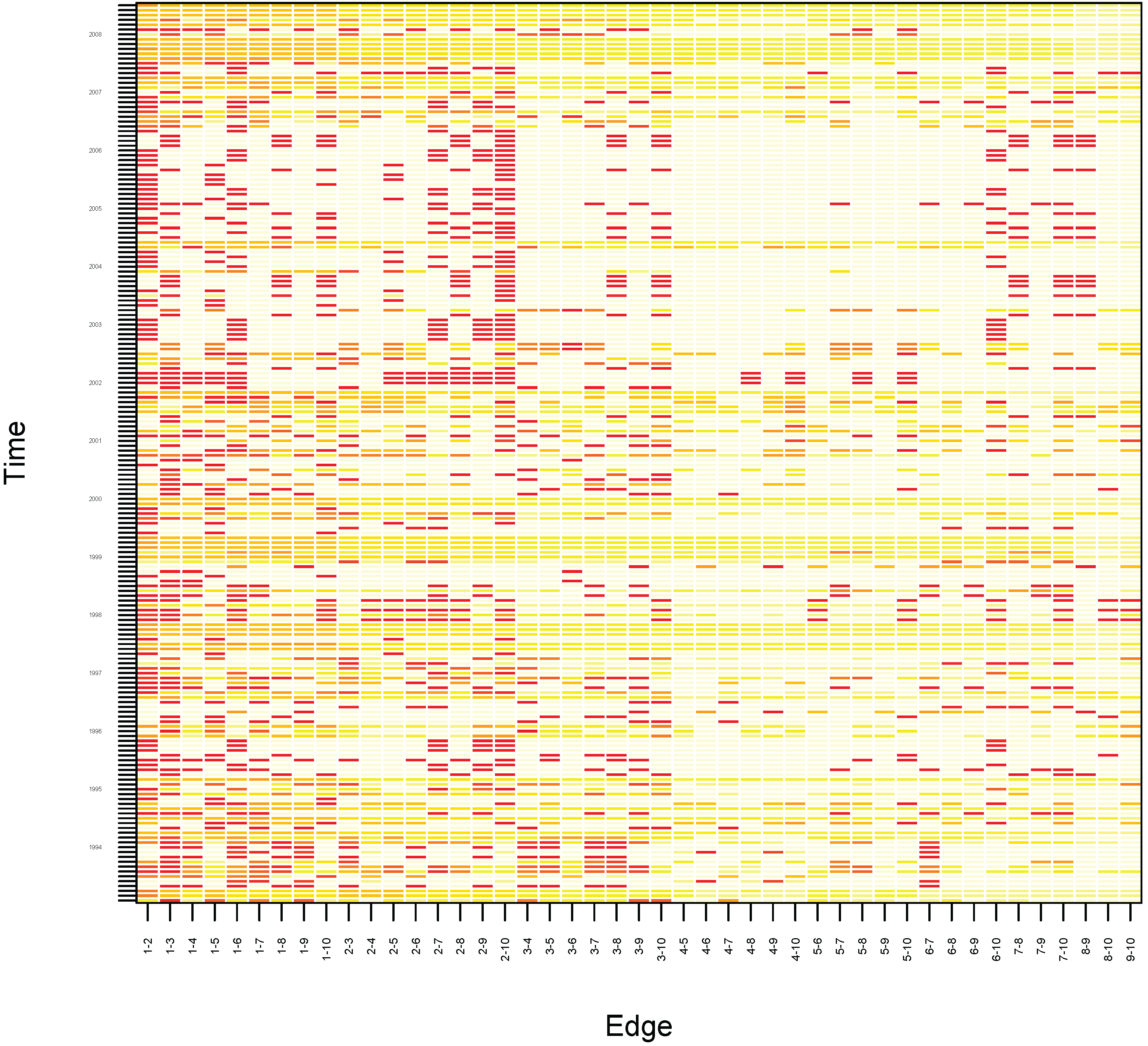
Figure 6 presents the Heatmap displaying the probability that two observations of edges of nine hedge fund strategy returns, the average for all strategies, and the seven factors from Fung and Hsieh’s [52] model belong to the same cluster between January 1994 and June 2009. The figure shows very high probabilities (more than 80%) that the following edges of hedge fund strategies belong to the same cluster during most of the months of the period January 1994 to June 2009, particularly during the bull market periods of 1994–1999 and 2003–2007:

• Short-bias and Event-Driven
• Short-bias and Fixed-Income
• Short-bias and Global Macro
• Short-bias and Managed Futures
• Emerging Markets and the bond market factor
• Emerging Markets and the commodity lookback straddle
• Event-Driven and the stock market factor
• Event-Driven and the firm size factor
• Event-Driven and the bond market factor
• Fixed-Income and Managed Futures
• Managed Futures and the firm size factor

Furthermore, and as expected, the probability that the Equity Market Neutral strategy and any other strategy belongs to the same cluster (except for the edge Equity Market Neutral and Short Bias during the second half of the sample period) is fairly low.

Fung and Hsieh [52] had already identified two breakpoints in factor exposures by hedge funds (September 1998, the collapse of LTCM, and March 2000, the beginning of the end of the Internet and technology bubble of the 1990s). This is consistent with hedge funds changing their strategies through time, this is, with alphas and betas being time-varying. Agarwal et al. [21] and Fung et al. [53] also use these breakpoints in their studies. Interestingly, [12] also report a structural break in the series of hedge fund returns in December of 2000.

The figure also illustrates that the global financial crisis of late 2008 (August through December), and the crisis experienced by financial markets in 1998 as a result of the Russian default and the LTCM debacle (September through November of that year) were two extraordinary events, because the probability that any two hedge fund strategies belonged to the same cluster was high, and almost the same for all the possible edges of hedge fund strategies during those two sub-periods, as can be seen by the lines of yellow/orange colors during those periods. This outlines the dangers from a risk management point of view of the presence of apparently uncorrelated groups of strategies or portfolios, that become highly correlated at periods of stress, due presumably to synchronized unwinding of positions across different strategies. These results also confirm the findings by [52], who had already reported a structural break in hedge fund index returns in September of 1998.

In a related article, [54] examine the extent to which hedge fund styles suffer from contagion. To that end, they use parametric and semi-parametric analysis and monthly hedge fund index data for the period 1990 to 2008. Contagion is defined as “correlation over and above what one would expect from economic fundamentals” (based on [55]). They find that hedge fund returns that fall in the bottom 10% of a hedge fund style’s monthly returns, cluster across styles. They also suggest that liquidity shocks to a number of contagion channel variables help explain hedge fund contagion.

6. Time-Varying Alphas and Betas Estimated Using iHMM-GGM

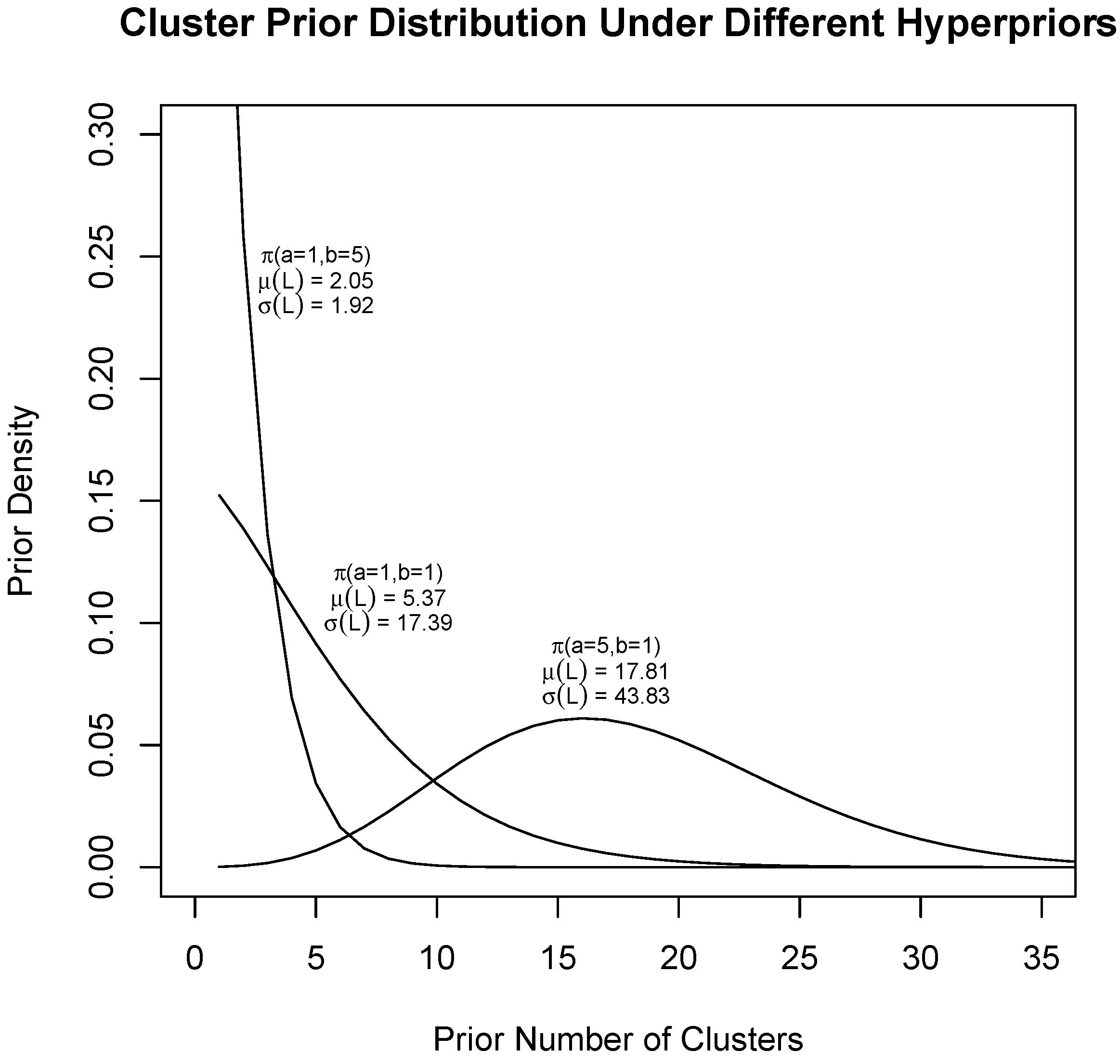
In this section we ran the model of [1] explained in Section 2 for 120,000 iterations and having descarted the first 20,000. The pseudo-code for computing the alpha and beta for each t = 1,...,186 consists in the following steps:

• For i = 1,...,120,000.
• Generate a value $L^i$ for the number of clusters in iteration i.
• Conditional on $L^i$, label each data vector ${\mathbf{z}}_t$ with a specific cluster ${\xi }_t^i$ so that ${\mathbf{z}}_{{\xi }_t^i}\sim \mathsf{N}({\mu }_{{\xi }_t^i},{\mathbf{K}}_{{\xi }_t^i}^{-1})$ for t = 1,...,186.
• Construct ${\alpha }_{{\xi }_t^i}={\mu }_{{\xi }_t^i}^y+{({\mathbf{K}}_{{\xi }_t}^{yy})}^{-1}{\mathbf{K}}_{{\xi }_t^i}^{yx}{\mu }_{{\xi }_t^i}^x$ and ${\beta }_{{\xi }_t^i}=-{({\mathbf{K}}_{{\xi }_t}^{yy})}^{-1}{\mathbf{K}}_{{\xi }_t^i}^{yx}$ for t = 1,...,186 from the distribution ${\mathbf{y}}_t|{\mathbf{x}}_t\sim \mathsf{N}\left({\mu }_{{\xi }_t}^y-{({\mathbf{K}}_{{\xi }_t}^{yy})}^{-1}{\mathbf{K}}_{{\xi }_t}^{yx}\left\{{\mathbf{x}}_t-{\mu }_{{\xi }_t}^x\right\},{({\mathbf{K}}_{{\xi }_t}^{yy})}^{-1}\right)$.
• For a given t, average over all clusters ${\xi }_t^i$ the values of ${\alpha }_{{\xi }_t^i}$ and ${\beta }_{{\xi }_t^i}$ as ${\alpha }_t=1/100,000{\sum }_{i=1}^{100,000}{\alpha }_{{\xi }_t^i}$ and ${\beta }_t=1/100,000{\sum }_{i=1}^{100,000}{\beta }_{{\xi }_t^i}$

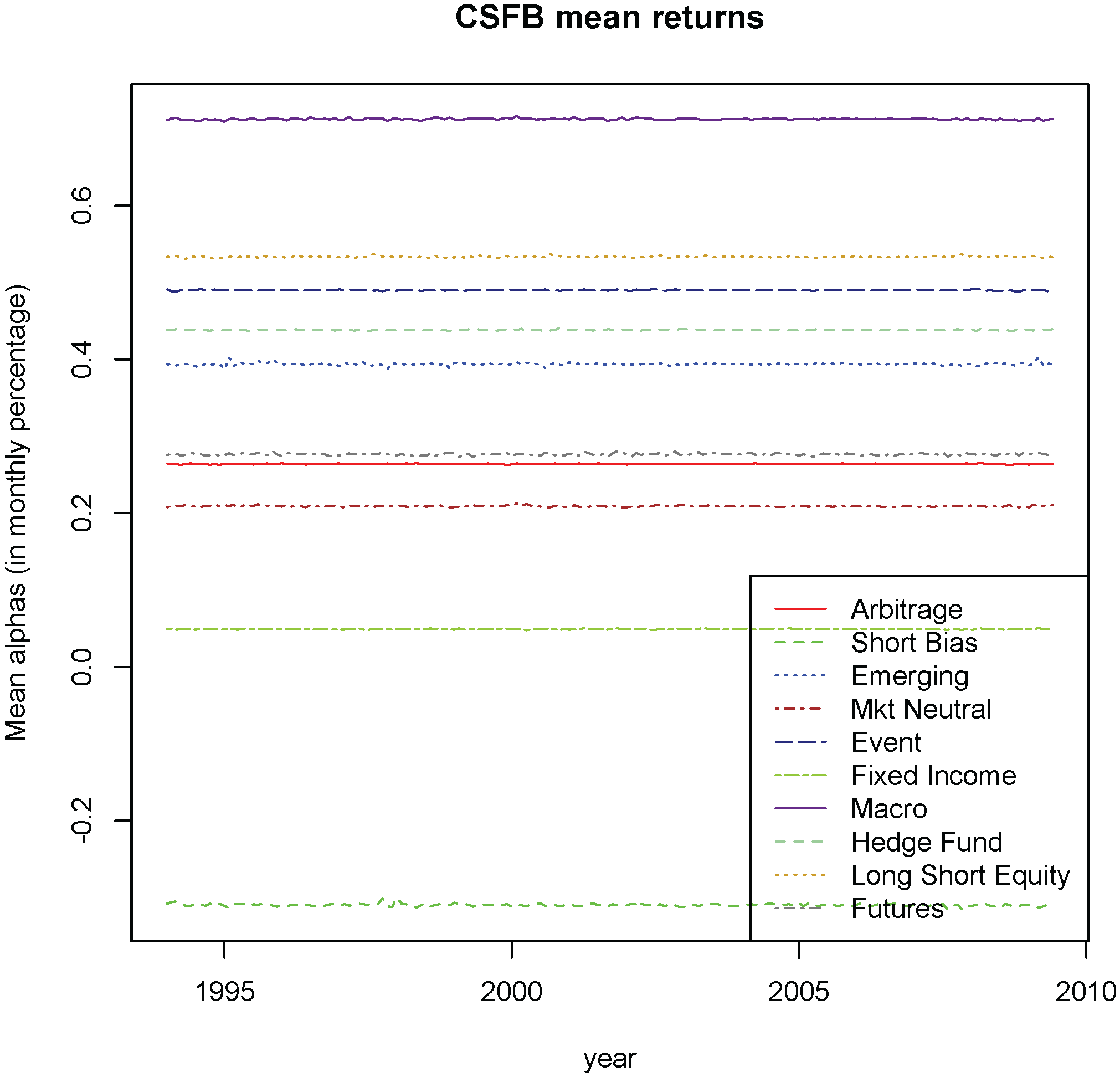
Figure 7 present the estimated mean alphas for each strategy from highest to lowest (in percent per month) and for the whole sample period: (1) Global Macro (1.02%); (2) Long/Short Equity (0.83%); (3) Event Driven (0.79%); (4) Emerging Markets (0.70%); (5) Managed Futures (0.58%); (6) Convertible Arbitrage (0.57%); (7) Equity Market Neutral (0.52%); (8) Fixed-Income (0.35%); and (9) Short-Bias (−0.02%).

Our results can be compared to those reported in a recent paper by [56], who also used a similar sample period (January 1995 to December 2009 versus our sample period of January 1994 to June 2009), and also worked with Fung and Hsieh’s seven factor model, but based their study on data from individual hedge funds available in TASS (we used CSFB/Tremont hedge fund indices) to estimate alpha applying OLS regressions. Ibbotson et al. [56] found a positive alpha for all strategies, although it was only statistically significant for the following strategies: equity market neutral (annualized alpha equal to 2.38%), event driven (annualized alpha equal to 3.73%), fixed income (annualized alpha equal to 2.39%), and long/short equity (annualized alpha equal to 5.16%). The average hedge fund had a statistically significant alpha of 3.01% per year. In our study, average hedge fund alpha was substantially higher, around 0.75% per month or 9.4% when annualized.

We also computed the difference between our estimated iHMM-GGM time-varying alphas for the nine CSFB/TREMONT hedge fund strategies and the average for all strategies, and the alphas estimated using OLS regressions during the sample period. We found that for all hedge fund strategies, except for Short-Bias (−0.6% per month), Managed Futures (−0.08% per month), and Fixed-Income (−0.04% per month), the difference between our estimated iHMM-GGM time-varying alphas and the estimated alphas using OLS regressions was positive on average. The highest difference was for Emerging Markets and Long/Short, at around 0.25% per month for each. The average hedge fund had an alpha that was around 0.13% per month (1.6% per year) higher when estimated using our iHMM-GGM procedure and the estimated alphas using OLS regressions. This implies that, over the time period we are using, estimations of alpha using OLS regressions such as those conducted in most of the prior research could underestimate the true alpha generated by the average hedge fund belonging to these three strategies. In

Table 5. Alpha volatilites over all the 186 periods for all the 10 strategies (standard deviations, monthly percentage). Source: Datastream, David Hsieh’s website, and own calculations.

CA	SB	EM	EMN	ED	FI	GM	HF	LS	F
0.322	0.150	0.240	0.118	0.446	0.486	1.010	0.507	0.229	0.502

we report the standard deviations of the 186 time-varying alphas for each of the nine strategies and for the average of all strategies. It is important to notice that computing the standard deviation over the 186 time- varying alphas only makes sense if we assume that these 186 alphas are each independent and identically distributed, something that we have seen is not the case since they are likely to be time-varying and not identically distributed (given the fact that they come estimated from our iHMM-GMM model). However, we still decided to report the standard deviations to have an idea of the variability of the alphas over all the 186 periods.

Global macro strikes out as the strategy having the most volatile alpha, around twice the volatility of that for managed futures, the second most volatile strategy in terms of alpha. This finding may be explained, in part, by the effect on the performance of global macro that had extraordinary events such as those of September 1998, in which Long Term Capital Management, a hedge fund belonging to this strategy and one of the largest hedge funds at the time, collapsed. As expected, the volatility of alpha for equity market neutral and long-short hedge funds is relatively low. The average performance of these strategies, especially in the case of equity market neutral, is more predictable and stable. The volatilities of alpha for event driven, convertible arbitrage and fixed-income strategies are close to the average volatility of all strategies. The volatility of alpha for emerging markets, a strategy that is in many respects similar to global macro, and short-bias hedge funds were around the lowest.

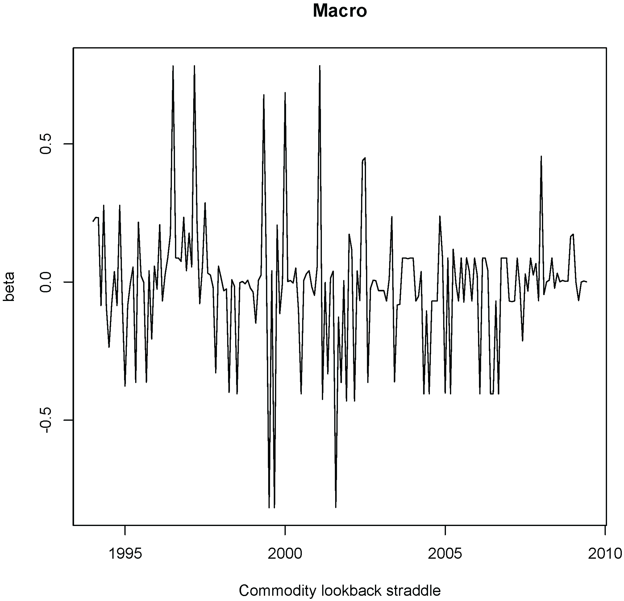
Figure 8 shows the estimated iHMM-GGM monthly alpha for the Global Macro Strategy estimated using the seven factor model for the whole sample period. For illustrative purposes, we chose to present here these time-varying alphas only for one of the strategies, Global Macro, which, as was just explained, was found to have the most volatile alpha of the nine strategies. The figure shows the volatility exhibited by the alpha of Global Macro. This volatility of the alphas questions the constant alpha assumption implicit in the estimation through regression models. We also present, in Figure 9, and for illustrative purposes, the estimated iHMM-GGM beta of the Global Macro Strategy with respect to one of the seven factors of Fung and Hsieh [52], the commodity lookback straddle factor, using the whole sample period. It can be clearly observed the high volatility of beta for Global Macro with respect to this specific factor, particularly during the first half of the sample period.

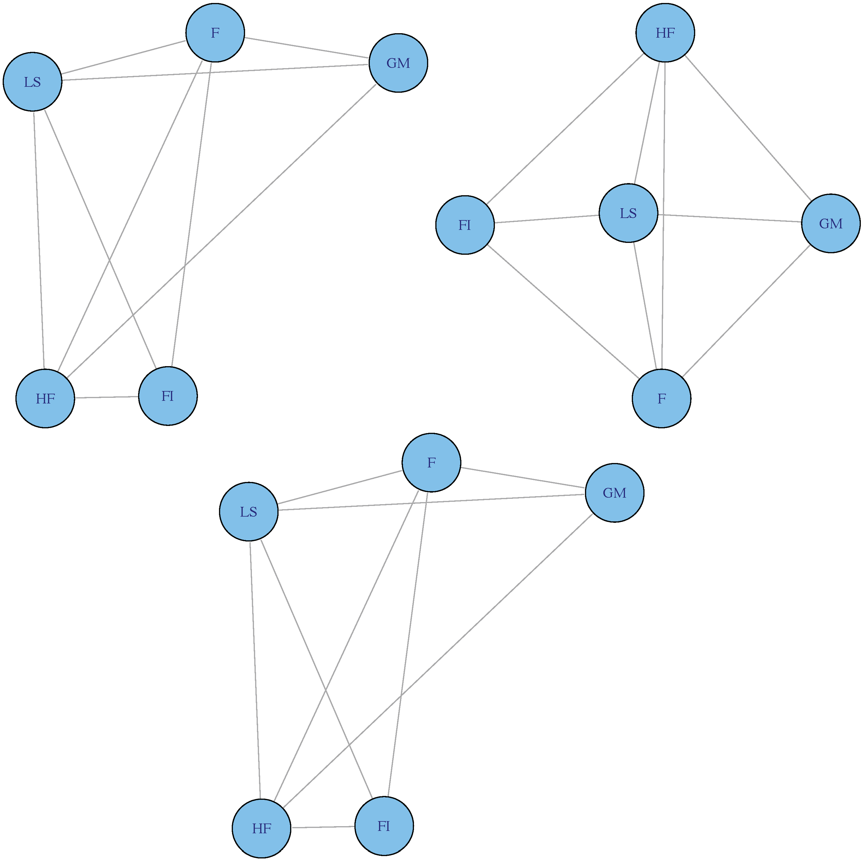
Figure 10 shows the graphical models associated to three critical time-points (months) during the sample: September 1998 (collapse of Long-Term Capital Management), March 2000 (beginning of the end of the 1990s bull market), and September 2008 (fall of Lehman Brothers and beginning of the global financial crisis). These graphs were built by adding any edge that had a greater than 80% posterior inclusion probability for the respective timepoint. It is striking to note that the three graphs are exactly the same, this is, they depict the same relation among four hedge fund strategies (global macro, fixed income, long/short and managed futures) and the average of the hedge fund indices for all strategies. The graphs suggest that in times of market crisis the aforementioned strategies belonged to the same cluster as they exhibited a high degree of covariation and dependence. Our findings from Figure 10 could be very useful, for example, for funds of hedge funds (or any other allocators), as they indicate that in times of market distress hedge funds dedicated to these strategies may suffer heavy losses and, thus, allocators investing into these categories of hedge funds will not be as diversified as originally thought. We can compare our results to previous studies. For example, Khandani and Lo [57], who also used CSFB/TREMONT hedge fund indices, documented that the global macro strategy had a correlation of only between 25% and 50% with both the long/short and the fixed income strategies between the following two sub-periods: April of 1994 to December of 2000, and January of 2001 to June of 2007; and that the fixed income strategy had a correlation of less than 25% with the long/short strategy during the same sub-periods. However, Figure 10 strongly suggests that the global macro and fixed income strategies were both linked to the long/short strategy but not between them during those months of market stress, and that the managed futures strategy was linked to the other three strategies. In turn, [57] also find, contrary to our results, a strong correlation (greater than 50%) between 29 pairs of hedge fund strategies and during the same sub-periods. Thus, our results may also uncover the dangers of inferring the benefits of diversifying into specific hedge funds styles in times of market crisis when using traditional correlation analysis. In sum, the understanding of the joint distribution of hedge fund styles under different clusters provides a portfolio view of their marginal impact and behavior. For example, if one identifies a crisis cluster and observes the inferred distribution of returns in that cluster, one may be able to construct a portfolio that weights funds more appropriately, not according to their Sharpe or other performance measures, but around the expected behavior of the distribution in times of crisis. Our findings are also important in the context of stress testing of portfolios during periods of market turmoil.

7. Conclusions and Extensions

We expand a novel statistical method to compute nonparametric dynamic alphas and betas, as well as returns clusters in a Bayesian fashion. This model provides a nonparametric, nonstationary, fully flexible approach to modelling sets of complex relationships between return series, regardless of the data generating process. We show through a simulation exercise that for both alpha and beta the estimation results based on the RMSE and MAD measures improve significantly upon popular statistical methods such as the regular OLS and DLMs, a special case of which being the Kalman filter. In a second exercise, we use hedge fund index returns from CSFB/Tremont for the period January 1994 to June 2009 and find that, using a Gaussian Graphical Model applied to Fung and Hsieh’s [52] seven-factor model, our estimated alphas are, on average, 0.75% per month. The average alphas of global macro, long/short equity and event driven were above the average for all strategies. The other strategies still had positive alphas, except for short-bias, although their average alphas were below the average for all strategies. Our estimated average alphas for all strategies are 0.13% per month (1.6% per year) higher than the alphas for all strategies estimated through OLS for the same period and, thus, our methodology reveals that average hedge fund alpha could be underestimated when measured using OLS. Furthermore, our estimated alphas and betas exhibit high volatility, particularly in periods which can be identified as times of stressful market events. Consistent with previous research, hedge fund returns were found to be non-normal. We also found that estimated alphas for the global macro strategy were highly volatile. The alphas of equity market neutral, long/short equity and emerging markets exhibited the lowest volatilities of the nine strategies. These findings question the use of parametric and stationary (non dynamic) models to estimate alphas and betas. The Bayesian procedure that we use in this paper has as advantages that it describes hedge fund returns in a dynamic, nonstationary and nonparametric form and, at the same time, allows us to extract new nonparametric, nonstationary and dynamic alphas and betas.

The procedure for measuring alpha that we propose in this paper was applied at the index level. Future research should investigate whether the same conclusions hold when individual hedge fund data is used. The use of individual hedge fund data also facilitates the measurement of performance persistence by grouping outperforming and underperforming hedged funds in each strategy and measuring their subsequent performance. Another extension would be to apply our procedure using other risk factors besides those of Fung and Hsieh [52] seven-factor model. In this regard, some authors have proposed specific factors for certain hedge fund strategies. For example, [58] propose a risk factor model for hedge funds dedicated to the fixed-income strategy. Finally, [21] document that mutual funds, which are catered mainly to small investors and are tightly regulated, as opposed to hedge funds, have recently begun offering funds that use trading strategies similar to those that are typical of hedge funds, as they include short sales and the use of derivatives, intended to take advantage of investment opportunities. These trading strategies should generate nonlinear payoffs and, thus, future research could also be extended to measuring mutual fund alpha using a more general procedure such as the one we propose here.

The focus of this paper has been on a descriptive approach to the returns for decision-makers. Future work will focus on forecasting, in cases where enough persistence exists in the series to provide sufficient structure. In this paper we do not presume that there is a stationary distribution to revert to, but instead a nonstationary process that reflects the less predictable characteristics of the returns.

One of the by-products of the methodology that we have presented in this paper is the time-varying probability that any two strategies belong to the same cluster. This information could be used by decision-makers in a number of different ways. For example, one approach would be through the understanding of the evolution of that relationship over time. However, another approach that could be more novel and meaningful, would be to analyze whether a set of strategies belong to the same cluster in key moments in time. Those key periods could be defined as periods with large negative returns, very large positive returns or any other particular feature that could be of relevance to the decision-maker, which in turn could help understand the relationship features between strategies with a higher granularity, as well as the expected marginal impact of additions to their portfolio in key periods. For example, Figure 10 showed that the graphical representation of the relationship between four specific strategies and aggregate hedge fund indices is the same in three key periods of time (September of 1998, March of 2000, and September of 2008). Whether the decision-maker expects that relationship to exist or expects further independence during times of market stress is outside the scope of this paper. However, the availability of this by-product brings in itself a significant number of areas of future research, including the analysis of the dynamics of these graphical structures over time and their impact on portfolio construction.

References

1. A. Rodriguez, A. Lenkoski, and A. Dobra. “Sparse covariance estimation in heterogeneous samples.” Electron. J. Stat. 5 (2011): 981–1014. [Google Scholar] [CrossRef]
2. S. Titman, and C. Tiu. “Do the Best Hedge Funds Hedge? ” Rev. Financ. Stud. 24 (2011): 123–168. [Google Scholar] [CrossRef]
3. H. Mamaysky, M. Spiegel, and H. Zhang. “Estimating the Dynamics of Mutual Fund Alphas and Betas.” Rev. Financ. Stud. 21 (2008): 233–264. [Google Scholar] [CrossRef]
4. W. Ferson, and R. Schadt. “Measuring Fund Strategy and Performance in Changing Economic Conditions.” J. Financ. 51 (1996): 425–461. [Google Scholar] [CrossRef]
5. A. Patton, and T. Ramadorai. “On the High-Frequency Dynamics of Hedge Fund Risk Exposures.” J. Financ. 68 (2013): 597–635. [Google Scholar] [CrossRef]
6. W. Fung, and D.A. Hsieh. “Hedge fund replication strategies: implications for investors and regulators.” Bank Fr. Financ. Stab. Rev.—Spec. Issue Hedge Funds 10 (2007): 55–66. [Google Scholar]
7. H. Kazemi, and T. Schneeweis. Conditional performance of hedge funds. CISDM Working Paper; Amherst, MA, USA: Center for International Securities and Derivatives Market, 2003. [Google Scholar]
8. M. Billio, M. Getmansky, and L. Pelizzon. “Dynamic risk exposures in hedge funds.” Comput. Stat. Data Anal. 56 (2012): 3517–3532. [Google Scholar] [CrossRef]
9. D.F. Ahelegbey, M. Billio, and R. Casarin. “Bayesian Graphical Models for Structural Vector Autoregressive Processes.” J. Appl. Econom., 2015. forthcoming. [Google Scholar] [CrossRef]
10. D. Bianchi, M. Billio, R. Casarin, and M. Guidolin. “Modeling Contagion and Systemic Risk.” Technical Report. 2015. Available online: http://ssrn.com/ abstract=2537986 (accessed on 22 February 2016).
11. R. Kosowski, N. Naik, and M. Teo. “Do hedge funds deliver alpha? A Bayesian and bootstrap analysis.” J. Financ. Econ. 84 (2007): 229–264. [Google Scholar] [CrossRef]
12. R. Kosowski, A. Timmermann, R. Wermers, and H. White. “Can mutual fund “stars” reallypick stocks? New evidence from a bootstrap analysis.” J. Financ. 61 (2006): 2551–2595. [Google Scholar] [CrossRef]
13. L. Pastor, and R. Stambaugh. “Investing in equity mutual funds.” J. Financ. Econ. 63 (2002): 351–380. [Google Scholar] [CrossRef]
14. W. Fung, and D.A. Hsieh. “The Risk in Hedge Fund Strategies: Theory and Evidence from Trend Followers.” Rev. Financ. Stud. 14 (2001): 313–341. [Google Scholar] [CrossRef]
15. M. Mitchell, and T. Pulvino. “Characteristics of Risk and Return in Risk Arbitrage.” J. Financ. 56 (2001): 2135–2176. [Google Scholar] [CrossRef]
16. V. Agarwal, and N. Naik. “Risk and portfolio decision involving hedge funds.” Rev. Financ. Stud. 17 (2004): 63–98. [Google Scholar] [CrossRef]
17. K.P. Baks, A. Metrick, and J. Wachter. “Should investors avoid all actively managed mutual funds? A study in Bayesian performance evaluation.” J. Financ. 56 (2001): 45–86. [Google Scholar] [CrossRef]
18. C.S. Jones, and J. Shanken. “Mutual fund performance with learning across funds.” J. Financ. Econ. 78 (2005): 507–552. [Google Scholar] [CrossRef]
19. D. Avramov, and R. Werner. “Investing in Mutual Funds when Returns are Predictable.” J. Financ. Econ. 81 (2006): 339–377. [Google Scholar] [CrossRef]
20. J. Busse, and P. Irvine. “Bayesian alphas and mutual fund persistence.” J. Financ. 61 (2006): 2251–2288. [Google Scholar] [CrossRef]
21. V. Agarwal, N. Boyson, and N.Y. Naik. “Hedge Funds for Retail Investors? An Examination of Hedged Mutual Funds.” J. Financ. Quant. Anal. 44 (2009): 273–305. [Google Scholar] [CrossRef]
22. A. Dempster. “Covariance selection.” Biometrics 28 (1972): 157–175. [Google Scholar] [CrossRef]
23. O. Aguilar, and M. West. “Bayesian Dynamic Factor Models and Portfolio Allocation.” J. Bus. Econ. Stat. 18 (2000): 338–357. [Google Scholar]
24. C.M. Carvalho, H.F. Lopes, and O. Aguilar. “Dynamic stock selection strategies: A structured factor model framework (with discussion).” In Bayesian Statistics 9. Edited by J.M. Bernardo, M. Bayarri, J.O. Berger, A. Dawid, D. Heckerman, A. Smith and M. West. Oxford, UK: Oxford University Press, 2011, pp. 69–90. [Google Scholar]
25. E.F. Fama, and K.R. French. “The Cross-Section of Expected Stock Returns.” J. Financ. 47 (1992): 427–465. [Google Scholar] [CrossRef]
26. E.F. Fama, and K.R. French. “Common risk factors in the returns on stocks and bonds.” J. Financ. Econ. 33 (1993): 3–56. [Google Scholar] [CrossRef]
27. M.M. Carhart. “On persistence in mutual fund performance.” J. Financ. 52 (1997): 57–82. [Google Scholar] [CrossRef]
28. C.M. Carvalho, and M. West. “Dynamic Matrix-Variate Graphical Models.” Bayesian Anal. 2 (2007): 69–98. [Google Scholar] [CrossRef]
29. A. Dobra, T. Eicher, and A. Lenkoski. “Modeling uncertainty in macroeconomic growth determinants using Gaussian graphical models.” Stat. Methodol. 7 (2010): 292–306. [Google Scholar] [CrossRef]
30. H. Wang. “Sparse Seemingly Unrelated Regression Modelling: Applications in Econometrics and Finance.” Comput. Stat. Data Anal. 54 (2010): 2866–2877. [Google Scholar] [CrossRef]
31. H. Wang, C. Reeson, and C.M. Carvalho. Dynamic Financial Index Models: Modeling Conditional Dependencies via Graphs. Technical Report; Austin, TX, USA: McCombs School of Business, University of Texas, 2011. [Google Scholar]
32. G. Letac, and H. Massam. “Wishart distributions for decomposable graphs.” Ann. Stat. 35 (2007): 1278–1323. [Google Scholar] [CrossRef]
33. B. Jones, C. Carvalho, A. Dobra, C. Hans, C. Carter, and M. West. “Experiments in stochastic computation for high-dimensional graphical models.” Stat. Sci. 20 (2005): 388–400. [Google Scholar] [CrossRef]
34. A. Lenkoski, and A. Dobra. “Computational Aspects Related to Inference in Gaussian Graphical Models with the G-Wishart Prior.” J. Comput. Gr. Stat. 20 (2011): 140–157. [Google Scholar] [CrossRef]
35. A. Dobra, A. Lenkoski, and A. Rodríguez. “Bayesian inference for general Gaussian graphical models with application to multivariate lattice data.” J. Am. Stat. Assoc. 106 (2011): 1418–1433. [Google Scholar] [CrossRef]
36. C. Rasmussen, and C. Williams. Gaussian Processes for Machine Learning, 1 ed. Cambridge, MA, USA: MIT Press, 2006. [Google Scholar]
37. T.S. Ferguson. “A Bayesian Analysis of Some Nonparametric Problems.” Ann. Stat. 1 (1973): 209–230. [Google Scholar] [CrossRef]
38. T.S. Ferguson. “Prior Distributions on Spaces of Probability Measures.” Ann. Stat. 2 (1974): 615–629. [Google Scholar] [CrossRef]
39. Y.W. Teh, M.I. Jordan, M.J. Beal, and D.M. Blei. “Sharing Clusters among Related Groups: Hierarchical Dirichlet Processes.” J. Am. Stat. Assoc. 101 (2006): 1566–1581. [Google Scholar] [CrossRef]
40. J. Van Gael, Y. Saatci, Y.W. Teh, and Z. Ghahramani. “Beam sampling for the Infinite Hidden Markov Model.” In Proceedings of the 25th International Conference on Machine Learning (ICML), Helsinki, Finland, 5–9 July 2008.
41. S. Fruewirth-Schnatter. Finite Mixture and Markov Switching Models. New York, NY, USA: Springer, 2006. [Google Scholar]
42. C. Antoniak. “Mixtures of Dirichlet processes with applications to Bayesian nonparametric problems.” Ann. Stat. 2 (1974): 1152–1174. [Google Scholar] [CrossRef]
43. Y. Song. “Modelling Regime Switching and Structural Breaks with an Infinite Hidden Markov Model.” J. Appl. Econom. 29 (2014): 825–842. [Google Scholar] [CrossRef]
44. E. Fox, E. Sudderth, M. Jordan, and A. Willsky. “A Sticky HDP-HMM with Application to Speaker Diarization.” Ann. Appl. Stat. 5 (2011): 1020–1056. [Google Scholar] [CrossRef]
45. G. Petris, S. Petrone, and P. Campagnoli. Dynamic Linear Models with R, 2nd ed. Heidelberg, Germany: Springer, 2009. [Google Scholar]
46. M. West, and J. Harrison. Bayesian Forecasting and Dynamic Models, 2nd ed. Heidelberg, Germany: Springer, 1997. [Google Scholar]
47. T. Schneeweis, and R. Spurgin. “Multi-Factor Models of Hedge Fund, Managed Futures, and Mutual Fund Return and Risk Characteristics.” J. Altern. Invest. 1 (1998): 1–24. [Google Scholar] [CrossRef]
48. B. Liang. “On the performance of hedge funds.” Financ. Anal. J. 55 (1999): 72–85. [Google Scholar] [CrossRef]
49. W. Fung, and D.A. Hsieh. “Performance Characteristics of Hedge Funds and Commodity Funds: Natural vs. Spurious Biases.” J. Financ. Quant. Anal. 35 (2000): 291–307. [Google Scholar] [CrossRef]
50. W. Fung, and D.A. Hsieh. “The Risk in Hedge Fund Strategies: Theory and Evidence from Trend Followers.” Rev. Financ. Stud. 14 (2001): 313–341. [Google Scholar] [CrossRef]
51. V. Agarwal, and N.Y. Naik. “Multi-Period Performance Persistence Analysis of Hedge Funds.” J. Financ. Quant. Anal. 35 (2000): 327–342. [Google Scholar] [CrossRef]
52. W. Fung, and D.A. Hsieh. “Hedge Fund Benchmarks: A Risk Based Approach.” Financ. Anal. J. 60 (2004): 65–80. [Google Scholar] [CrossRef]
53. W. Fung, D.A. Hsieh, N. Naik, and T. Ramadorai. “Hedge Funds:Performance, Risk and Capital Formation.” J. Financ. 63 (2008): 1777–1803. [Google Scholar] [CrossRef]
54. N. Boyson, R. Stulz, and C. Stahel. “Hedge Fund Contagion and Liquidity Shocks.” J. Financ. 65 (2010): 1789–1816. [Google Scholar] [CrossRef]
55. G. Bekaert, C. Harvey, and A. Ng. “Market Integration and Contagion.” J. Bus. 78 (2005): 39–69. [Google Scholar] [CrossRef]
56. R.G. Ibbotson, P. Chen, and K.X. Zhu. “The ABCs of Hedge Funds: Alphas, Betas, and Costs.” Financ. Anal. J. 67 (2011): 15–25. [Google Scholar] [CrossRef]
57. A. Khandani, and A. Lo. “What Happened to the Quants in August 2007? ” J. Invest. Manag. 5 (2007): 29–78. [Google Scholar] [CrossRef]
58. W. Fung, and D.A. Hsieh. “The Risk in Fixed-Income Hedge Fund Styles.” J. Fixed Income 12 (2002): 6–27. [Google Scholar] [CrossRef]
Figure 1. The implied prior on L given a diferent set of hyperparameters values for a and b. This figure includes the distribution of three of those priors that represent a reasonable range for the problem at hand.
Econometrics 04 00013 g001
Figure 2. The posterior distribution of the parameter L (number of clusters) under the data described in Section 4 given a diferent set of hyperparameters values for a and b.
Econometrics 04 00013 g002
Figure 3. Stickyness of consecutive clusters.
Econometrics 04 00013 g003
Figure 4. Distribution of the number of clusters ( L ) for each of the series individually, versus the case of the joint modeling.
Econometrics 04 00013 g004
Figure 5. ACF and traceplot for parameter L (number of clusters).
Econometrics 04 00013 g005
Figure 6. (HeatmapEdgeChronoCSFBwithoutfactors file, 4 September 2011): Heatmap displaying the probability that two observations of nine hedge fund returns, the average for all strategies belong to the same cluster between January 1994 and June 2009. Source: Datastream, David Hsieh’s website, and own calculations. The notation used on the x-axis is as follows. CSFB/TREMONT Hedge Fund Strategies: 1: Convertible Arbitrage, 2: Short Bias, 3: Emerging Markets, 4: Equity Market Neutral, 5: Event-Driven, 6: Fixed-Income, 7: Global Macro, 8: Hedge Funds (all strategies), 9: Long-Short Equity, and 10: Managed Futures.
Econometrics 04 00013 g006
Figure 7. (mu file, 4 September 2011): Estimated mean alphas (in percent per month) of the nine CSFB/TREMONT hedge fund strategies and the average for all strategies (January 1994 to June 2009). Source: Datastream, David Hsieh’s website, and own calculations.
Econometrics 04 00013 g007
Figure 8. (CSGlobalMacroAlpha file, 4 September 2011): Estimated iHMM-GGM monthly alpha compared to alpha estimated from a linear regression for the Global Macro Strategy with respect to the seven factor model of Fung and Hsieh [52] (January 1994 to June 2009). Source: Datastream, David Hsieh’s website, and own calculations.
Econometrics 04 00013 g008
Figure 9. 6b (CSGlobalMacroBeta file, 4 September 2011): Estimated iHMM-GGM beta of the Global Macro Strategy with respect to the commodity lookback straddle factor of Fung and Hsieh ([52], January 1994 to June 2009). Source: Datastream, David Hsieh’s website, and own calculations.
Econometrics 04 00013 g009
Figure 10. The left graph is for September 2008, the center graph is for March 2000 and the right graph is for September 1998. Source: Datastream, David Hsieh’s website, and own calculations.
Econometrics 04 00013 g010