Evolutionary Sequential Monte Carlo Samplers for Change-Point Models

Abstract

Sequential Monte Carlo (SMC) methods are widely used for non-linear filtering purposes. However, the SMC scope encompasses wider applications such as estimating static model parameters so much that it is becoming a serious alternative to Markov-Chain Monte-Carlo (MCMC) methods. Not only do SMC algorithms draw posterior distributions of static or dynamic parameters but additionally they provide an estimate of the marginal likelihood. The tempered and time (TNT) algorithm, developed in this paper, combines (off-line) tempered SMC inference with on-line SMC inference for drawing realizations from many sequential posterior distributions without experiencing a particle degeneracy problem. Furthermore, it introduces a new MCMC rejuvenation step that is generic, automated and well-suited for multi-modal distributions. As this update relies on the wide heuristic optimization literature, numerous extensions are readily available. The algorithm is notably appropriate for estimating change-point models. As an example, we compare several change-point GARCH models through their marginal log-likelihoods over time.

1. Introduction

Sequential Monte Carlo (SMC) algorithm is a simulation-based procedure used in Bayesian frameworks for drawing distributions. Its core idea relies on an iterated application of the importance sampling technique to a sequence of distributions converging to the distribution of interest 1. For many years, on-line inference was the most relevant applications of SMC algorithms. Indeed, one powerful advantage of sequential filtering consists in being able to update the distributions of the model parameters in light of new coming data (hence the term on-line) allowing for an important time saving compared to off-line methods such as the popular Markov-Chain Monte-Carlo (MCMC) procedure that requires a new estimation based on all the data at each new observation entering in the system. Other SMC features making it very promising are an intuitive implementation based on the importance sampling technique ([1,2,3]) and a direct computation of the marginal likelihood (i.e., the normalizing constant of the targeted distribution, see, e.g., [4]).

Recently, the SMC algorithms have been applied to infer static parameters, field in which the MCMC algorithm excels. Neal [5] provides a relevant improvement in this direction by building a SMC algorithm, named annealed importance sampling (AIS), that sequentially evolves from the prior distribution to the posterior distribution using a tempered function, which basically consists in gradually introducing the likelihood information into the sequence of distributions by means of an increasing function. To preclude particles degeneracies, he uses an MCMC kernel at each SMC iteration. Few years later, [6] proposes an Iterated Batch Importance Sampling (IBIS) SMC algorithm, a special case of the Re-sample Move (RM) algorithm of [7], which sequentially evolves over time and adapts the posterior distribution using the previous approximate distribution. Again, an MCMC move (and a re-sampling step) is used for diversifying the particles. The SMC sampler (see [8]) unifies, among others, these SMC algorithms in a theoretical framework. It is shown that the methods of [5,7] arise as special cases with a specific choice of the ’backward kernel function’ introduced in their paper. These researches have been followed by empirical works (see [9,10,11]) where it is demonstrated that the SMC mixing properties often dominate the MCMC approach based on a single Markov-chain. Nowadays papers are devoted to build self-adapting SMC samplers by automatically tuning the MCMC kernel (e.g., [12]), by marginalizing the state vector (in a state space specification) using the particle MCMC framework (e.g., [13,14]), to construct efficient SMC samplers for parallel computations (see [15]) or to simulate from complex multi-modal posterior distributions (e.g., [16]).

In this paper, we document a generic SMC inference for change-point models that can additionally be updated through time. For example, in a model comparison context the standard methodology consists in repeating estimations of the parameters given an evolving number of observations. In circumstances where the Bayesian estimation is highly demanding as it is usually the case for complex models and where the number of available observations is huge, this iterative methodology can be too intensive. Change-point (CP) Generalized Autoregressive Conditional Heteroskedastic (GARCH) processes may require several hours for one inference (e.g., [17]). A recursive forecast exercise on many observations is therefore out of reach. Our first contribution is a new SMC algorithm, called tempered and time (TNT), which exhibits the AIS, the IBIS and the RM samplers as special cases. It innovates by switching over tempered and time domains for estimating posterior distributions. For instance, it firstly iterates from the prior to the posterior distributions by means of a sequence of tempered posterior distributions. It then updates in the time dimension the slightly different posterior distributions by sequentially adding new observations, each SMC step providing all the forecast summary statistics relevant for comparing models. The TNT algorithm combines the tempered approach of [5] with the IBIS algorithm of [6] if the model parameters are static or with the RM method of [7] if their support evolves with the SMC updates. Since all these methods are built on the same SMC steps (re-weighting, re-sampling and re-juvenating) and the same SMC theory, the combination is achieved without efforts.

The proposed methodology exhibits several advantages over SMC algorithms that directly iterate on the time domain ([6,7]). In fact, these algorithms may experience high particle discrepancies. Although the problem is more acute for models where the parameter space evolves through time, it remains an issue for models with static parameters at the very first SMC steps. To quote [6] (p. 546) :

Note that the particle system may degenerate strongly in the very early stages, when the evolving target distribution changes the most[...].

The combination of tempered and time SMC algorithms allows to limit this particle discrepancy observed at the early stage since the first posterior distribution of interest is estimated by taking into account more than a few observations. One advantage of using a sequence of tempered distributions to converge to the posterior distribution consists in the number of SMC steps that can be used. Compared to the SMC algorithms that directly iterate on time domain where the sequence of distributions is obviously defined by the number of data, the tempered approach allows for choosing this sequence of distribution and for targeting the posterior distribution of interest by using as many bridging distributions as needed.

Many SMC algorithms rely on MCMC kernels to rejuvenate the particles. The TNT sampler is no exception. We contribute by proposing several new generic MCMC kernels based on the heuristic optimization literature. These kernels are well appropriated in the SMC context as they build their updates on the particles interactions. We start by emphasizing that the DiffeRential Evolution Adaptive Metropolis (DREAM, see [18]), the walk move (see [19]) and the stretch one (see [20]) separately introduced in the statistic literature as generic Metropolis-Hastings proposals are in fact standard mutation rules of the Differential Evolution (DE) optimization. From this observation, we propose seven new MCMC updates based on the heuristic literature and emphasize that many other extensions are possible. The proposed MCMC kernel is adapted for continuous parameters. Consequently, discrete parameters such as the break parameters of change-point models cannot directly be inferred from our algorithm. To solve this issue, we transform the break parameters into continuous ones which make them identifiable up to a discrete value. To illustrate the potential of the TNT sampler, we compare several CP-GARCH models differing by their number of regimes on the S&P 500 daily percentage returns.

The paper is organized as follows. Section 2 presents the SMC algorithm as well as its theoretical derivation. Section 3 introduces the different Metropolis-Hastings proposals which compose what we call the Evolutionary MCMC. We then detail a simulation exercise on the CP-GARCH process in Section 4. Eventually we study the CP-GARCH performance on the S&P 500 daily percentage returns in Section 5. Section 6 concludes.

2. Off-line and On-Line Inferences

We first theoretically and practically introduce the tempered and time (TNT) framework. To ease the discussion, let us consider a standard state space model:

$$\begin{array}{ccc}\hfill y_t& =& f(\theta ,s_t,{\omega }_t)\hfill \end{array}$$

(1)

$$\begin{array}{ccc}\hfill s_t& =& g(\theta ,s_{t-1},v_t)\hfill \end{array}$$

(2)

where $s_t$ is a random variable driven by a Markov chain and the functions f(-) and g(-) are deterministic given their arguments. The observation $y_t$ belongs to the set $y_{1:T}=\{y_1,...,y_T\}$ with T denoting the sample size and is assumed to be independent conditional to the state $s_t$ and θ with distribution $f(y_t|\theta ,s_t)$. The innovations ${\omega }_t$ and $v_t$ are mutually independent and stand for the noise of the observation/state equations. The model parameters included in θ do not evolve over time (i.e., they are static). Let us denote the set of parameters at time t by $x_t=\{\theta ,s_{1:t}\}$ defined on the measurable space $E_t$.

We are interested in estimating many posterior distributions starting from $\pi (x_{\tau }|y_{1:\tau })$, where $\tau <<T$, until T. The SMC algorithm approximates these posterior distributions with a large (dependent) collection of M weighted random samples ${\{W_t^i,x_t^i\}}_{i=1}^M$ where $W_t^i>0\text{and}{\sum }_{i=1}^M{W}_t^i=1$ such that as $M\to \infty$, the empirical distribution converges to the posterior distribution of interest, meaning that for any $\pi (x_t|y_{1:t})$-integrable function g : $E_t\to \Re$:

$$\sum _{i=1}^M{W}_t^{i}g(x_t^i)\to {\int }_{E_t}g(x_t)\pi (x_t|y_{1:t})d{x}_t\text{almost}\text{surely}.$$

The TNT method combines an enhanced Annealed Importance sampling 2 (AIS, see [5]) with the Re-sample Move (RM) SMC inference of [7] 3. To build the TNT algorithm, we rely on the theoretical paper of [8] that unifies the two SMC methods into one SMC framework called “SMC sampler”. The TNT algorithm first estimates an initial posterior distribution, namely $\pi (x_{\tau }|y_{1:\tau })$, by an enhanced AIS (E-AIS) algorithm and then switches from the tempered domain to the time domain and sequentially updates the approximated distributions from $\pi (x_{\tau }|y_{1:\tau })$ to $\pi (x_T|y_{1:T})$ by adding one by one the new observations. We now begin by mathematically deriving the validity of the SMC algorithms under the two different domains and by showing that they are particular cases of the SMC sampler. The practical algorithm steps are given afterward (see Subsection 2.3).

2.1. E-AIS : The Tempered Domain

The first phase, carried out by an E-AIS, creates a sequence of probability measures ${\{{\pi }_n\}}_{n=0}^p$ that are defined on the measurable spaces $\{E_n,{\xi }_n\}$, where $E_n=E_{n+1}=E\ni x_{\tau }$, $n\in \{0,1,...,p\}$ is a counter and does not refer to ’real time’, p denotes the number of posterior distribution estimations and ${\pi }_p$ coincides with the first posterior distribution of interest $\pi (x_{\tau }|y_{1:\tau })$. The sequence distribution, used as bridge distributions, is defined as ${\pi }_n(x_n|y_{1:\tau })=\gamma {(y_{1:\tau }|x_n)}^{\varphi (n)}f(x_n)/Z_n$ where $Z_n={\int }_E\gamma {(y_{1:\tau }|x_n)}^{\varphi (n)}f(x_n)d{x}_n$ denotes the normalizing constant, $\gamma (y_{1:\tau }|x_n)$ and $f(x_n)$ respectively are the likelihood function and the prior density of the model. Through an increasing function $\varphi (n)$ respecting the bound conditions $\varphi (0)=0$ and $\varphi (p)=1$, the E-AIS artificially builds a sequence of distributions that converges to the posterior distribution of interest.

Remark 1: The random variables ${\{x_n\}}_{n=0}^p$ exhibit the same support E which is also shared by $x_{\tau }$. Furthermore, the random variable $x_{\tau }$ coincides with $x_p$ since $\varphi (p)=1$.

The E-AIS is merely a sequential importance sampling technique where the draws of a proposal distribution ${\eta }_n$ combined with an MCMC kernel are used to approximate the next posterior distribution ${\pi }_{n+1}$, the difficulty lying in specifying the sequential proposal distribution. Del Moral, Doucet, and Jasra [8] theoretically develop a coherent framework for choosing a generic sequence of proposal distributions.

In the SMC sampler framework, we augment the support of the posterior distribution ensuring that the targeted posterior distribution marginally arises :

$$\begin{array}{ccc}\hfill {\tilde{\pi }}_n(x_{1:n})& =& {\pi }_n(x_n)\prod _{k=2}^n{L}_k(x_{k-1}|x_k),\hfill \\ & =& \frac{{\gamma }_n(x_n)}{Z_n}\prod _{k=2}^n{L}_k(x_{k-1}|x_k),\hfill \end{array}$$

where ${\gamma }_n(x_n)=\gamma {(y_{1:\tau }|x_n)}^{\varphi (n)}f(x_n)$, $Z_n={\int }_E\gamma {(y_{1:\tau }|x_n)}^{\varphi (n)}f(x_n)d{x}_n$ is the normalizing constant, and $L_k(x_{k-1}|x_k)$ is a backward MCMC kernel such that ${\int }_E{L}_k(x_{k-1}|x_k)d{x}_{k-1}=1$.

By defining a sequence of proposal distributions as

$$\begin{array}{ccc}\hfill {\eta }_n(x_{1:n})& =& f(x_1)\prod _{k=2}^n{K}_k(x_k|x_{k-1}),\hfill \end{array}$$

where $K_k(x_k|x_{k-1})$ is an MCMC kernel with stationary distribution ${\pi }_k$ such that it verifies ${\pi }_k(x_k)={\int }_E{K}_k(x_k|x_{k-1}){\pi }_k(x_{k-1})d{x}_{k-1}$, we derive a recursive equation of the importance weight:

$$\begin{array}{ccc}\hfill w_n(x_{1:n})& =& \frac{{\gamma }_n(x_n){\prod }_{k=2}^n{L}_k(x_{k-1}|x_k)}{Z_{n}f(x_1){\prod }_{k=2}^n{K}_k(x_k|x_{k-1})},\hfill \\ & =& w_{n-1}(x_{1:n-1})\frac{Z_{n-1}{\gamma }_n(x_n)L_n(x_{n-1}|x_n)}{Z_n{\gamma }_{n-1}(x_{n-1})K_n(x_n|x_{n-1})}.\hfill \end{array}$$

For a smooth increasing tempered function $\varphi (n)$, we can argue that ${\pi }_{n-1}$ will be close to ${\pi }_n$. W therefore define the backward kernel by detailed balance argument as

$$\begin{array}{c}\hfill L_n(x_{n-1}|x_n)=\frac{{\pi }_n(x_{n-1})}{{\pi }_n(x_n)}{K}_n(x_n|x_{n-1}).\end{array}$$

(3)

It gives the following weights :

$$\begin{array}{ccc}\hfill w_n(x_{1:n})& =& w_{n-1}(x_{1:n-1})\frac{Z_{n-1}{\gamma }_n(x_{n-1})}{Z_n{\gamma }_{n-1}(x_{n-1})},\hfill \\ & \propto & w_{n-1}(x_{1:n-1})\gamma {(y_{1:\tau }|x_{n-1})}^{{\varphi }_n-{\varphi }_{n-1}}.\hfill \end{array}$$

(4)

The normalizing constant $Z_n$ is approximated as

$$\frac{Z_n}{Z_{n-1}}\approx \sum _{i=1}^M{W}_{n-1}^i\frac{{\gamma }_n(x_{n-1}^i)}{{\gamma }_{n-1}(x_{n-1}^i)},$$

where $W_{n-1}^i=w_{n-1}(x_{1:n-1}^i)/{\sum }_{j=1}^M{w}_{n-1}(x_{1:n-1}^j)$, i.e., the normalized weight.

The E-AIS requires to tune many parameters : an increasing function $\varphi (n)$, the MCMC kernels with the invariant distributions ${\pi }_n(.)$, a number of particles M, of iterations p, of MCMC steps J. Adjusting these parameters can be difficult. Some guidance are given in [16] for DSGE models. For example, they propose a quadratic tempered function $\varphi (n)$. It slowly increases for small values of n and the step becomes larger and larger as n tends to p. In this paper, the TNT algorithm generically adapts the different user-defined parameters and belongs to the class of adaptive SMC algorithms. It automatically adjusts the tempered function with respect to an efficiency measure as it was proposed by [10]. By doing so, we preclude the difficult choice of the function $\varphi (n)$ and the number of iteration p. The number of MCMC steps J will be controlled by the acceptance rate exhibited by the MCMC kernels. The choice of MCMC kernels and the number of particles are discussed later (see Section 3).

2.2. The Re-Sample Move Algorithm : The Time Domain

Once we have a set of particles that approximates the first posterior distribution of interest $\pi (x_{\tau }|y_{1:\tau })$, a second phase takes place. Firstly, let us assume that the support of $x_t$ does not evolve over time (i.e., $x_t\in E\forall t$). In this context, the SMC sampler framework shortly reviewed here for the tempered domain still applies. Let us define the following distributions:

$$\begin{array}{ccc}\hfill {\pi }_t(x_t)& =& \pi (x_t|y_{1:t}),\hfill \\ \hfill {\tilde{\pi }}_t(x_{1:t})& =& {\pi }_t(x_t)\prod _{k=2}^t{L}_k(x_{k-1}|x_k),\hfill \\ \hfill {\eta }_t(x_{1:t})& =& f(x_1)\prod _{k=2}^t{K}_k(x_k|x_{k-1}),\hfill \\ \hfill L_k(x_{k-1}|x_k)& =& \frac{{\pi }_k(x_{k-1})}{{\pi }_k(x_k)}{K}_k(x_k|x_{k-1}).\hfill \end{array}$$

Then the weight equation of the SMC sampler is equal to

$$\begin{array}{ccc}\hfill w_t(x_{1:t})& =& w_{t-1}(x_{1:t-1})\frac{{\pi }_t(x_{t-1})}{{\pi }_{t-1}(x_{t-1})},\hfill \end{array}$$

(5)

which is exactly the weight equation of the IBIS algorithm (see [6], step 1, p. 543).

Let now consider the more difficult case where a subset of the support of $x_t$ evolves with t such as $x_t=\{x_{t-1},s_t\}=\{\theta ,s_{1:t-1},s_t\}$ (see the state space model Equations (1) and (2)) meaning that $\forall t\in [1,T],x_t\in E_t$ and $E_{t-1}\subset E_t$. The previous method cannot directly be applied (due to the backward kernel) but with another choice of the kernel functions, the SMC sampler also operates. Let us define the following distribution :

$$\begin{array}{ccc}\hfill {\pi }_t(x_t)& =& \pi (x_t|y_{1:t}),\hfill \end{array}$$

(6)

$$\begin{array}{ccc}\hfill {\tilde{\pi }}_t(x_{1:t},x_{2:t}^{*})& =& {\pi }_t(x_t)\prod _{k=2}^t{L}_k(x_{k-1},x_k^{*}|x_k),\hfill \end{array}$$

(7)

$$\begin{array}{ccc}\hfill {\eta }_t(x_{1:t},x_{2:t}^{*})& =& f(x_1)\prod _{k=2}^t{\tilde{K}}_k(x_k,x_k^{*}|x_{k-1}),\hfill \end{array}$$

(8)

$$\begin{array}{ccc}\hfill {\tilde{K}}_k(x_k,x_k^{*}|x_{k-1})& =& {\tilde{q}}_k(x_k^{*}|x_{k-1})K_k(x_k|x_k^{*}),\hfill \end{array}$$

(9)

$$\begin{array}{ccc}\hfill L_k(x_{k-1},x_k^{*}|x_k)& =& q_k(x_{k-1}|x_k^{*})K_k(x_k^{*}|x_k),\hfill \end{array}$$

(10)

$$\begin{array}{ccc}\hfill K_k(x_k^{*}|x_k)& =& \frac{{\pi }_k(x_k^{*})K_k(x_k|x_k^{*})}{{\pi }_k(x_k)}\text{by}\text{detailed}\text{balance}\text{argument}.\hfill \end{array}$$

(11)

To deal with the time-varying dimension of $x_t$, we augment the support of the artificial sequence of distributions by several new random variables (see $x_{2:t}^{*}$ in Equation (7)) while ensuring that the posterior distribution of interest ${\pi }_t(x_t)$ marginally arises. Sampling from the proposal distribution ${\eta }_t(x_{1:t},x_{2:t}^{*})$ is achieved by drawing from the prior distribution and then by sequentially sampling from the distributions ${\tilde{K}}_k(x_k,x_k^{*}|x_{k-1})$, which are composed by a user-defined distribution ${\tilde{q}}_k(x_k^{*}|x_{k-1})$ and an MCMC kernel exhibiting ${\pi }_k(x_k)$ as the invariant distribution.

Under this framework, the weight equation of the SMC sampler becomes

$$\begin{array}{ccc}\hfill w_t(x_{1:t},x_{2:t}^{*})& =& w_{t-1}(x_{1:t-1},x_{2:t-1}^{*})\frac{{\pi }_t(x_t^{*})q_t(x_{t-1}|x_t^{*})}{{\pi }_{t-1}(x_{t-1}){\tilde{q}}_t(x_t^{*}|x_{t-1})}.\hfill \end{array}$$

(12)

By setting the distributions $q_t(x_{t-1}|x_t^{*})={\delta }_{\{x_{t-1}={\theta }^{*},s_{1:t-1}^{*}\}}$, where ${\delta }_i$ denotes the probability measure concentrated at i, and ${\tilde{q}}_t(x_t^{*}|x_{t-1})={\nu }_t(s_t^{*}|x_{t-1}){\delta }_{\{{\theta }^{*},s_{1:t-1}^{*}=x_{t-1}\}}$, we recover the weight equation of [7] (see Equation (20), p. 135)

$$\begin{array}{ccc}\hfill w_t(x_{1:t},x_{2:t}^{*})& =& w_{t-1}(x_{1:t-1},x_{2:t-1}^{*})\frac{{\pi }_t(x_{t-1},s_t^{*})}{{\pi }_{t-1}(x_{t-1}){\nu }_t(s_t^{*}|x_{t-1})}.\hfill \end{array}$$

(13)

Like in [7], only the distribution ${\nu }_t(.)$ has to be specified. For example, it can be set either to the prior distribution or the full conditional posterior distribution (if the latter exhibits a closed form).

Remark 2: The division $\frac{\pi (x_t|y_{1:t})}{\pi (x_{t-1}|y_{1:t-1})}$ appearing in the weight Equations ((5) and (13)) can be reduced to $\frac{Z_{t-1}}{Z_t}\gamma (y_t|x_t,y_{1:t-1})f(s_t|x_{t-1})$ which highly limits the computational cost of the weights.

2.3. The TNT Algorithm

The algorithm initializes the M particles using the prior distributions, sets each initial weight ${\{W_0^i\}}_{i=1}^M$to $W_0^i=\frac{1}{M}$ and then iterates from $n=1,\dots ,p,p+1,...,p+(T-\tau )+1$ as follows

• Correction step: $\forall i\in [1,M]$, Re-weight each particle with respect to the nth posterior distribution

  –

  If in tempered domain ( $n\le p$ ) :

  $$\begin{array}{c}\hfill {\tilde{w}}_n^i=\gamma {(y_{1:\tau }|x_{n-1}^i)}^{\varphi (n)-\varphi (n-1)}\end{array}$$

  (14)

  –

  If in time domain ( $n>p$ ) and the parameter space does not evolve over time (i.e., $E_{n-1}=E_n$) :

  $$\begin{array}{c}\hfill {\tilde{w}}_n^i=\frac{\gamma (y_{1:\tau +n-p}|x_{n-1}^i)}{\gamma (y_{1:\tau +n-p-1}|x_{n-1}^i)}=\gamma (y_{\tau +n-p}|x_{n-1}^i,y_{1:\tau +n-p-1})(\text{see}\text{remark}2)\end{array}$$

  (15)

  –

  If in time domain ( $n>p$ ) and the parameter space increases (i.e., $E_{n-1}\subset E_n$) :

  Set $x_n^i=\{x_{n-1}^i,s_n^i\}$ with $s_n^i\sim {\nu }_n(.|x_{n-1}^i)$.

  $$\begin{array}{c}\hfill {\tilde{w}}_n^i=\frac{\gamma (y_{1:\tau +n-p}|x_n^i)f(x_n^i)}{\gamma (y_{1:\tau +n-p-1}|x_{n-1}^i)f(x_{n-1}^i){\nu }_n(s_n^i|x_{n-1}^i)}\end{array}$$

  (16)

  Compute the unnormalized weights : ${\tilde{W}}_n^i={\tilde{w}}_n^i{W}_{n-1}^i$.
  Normalize the weights : $W_n^i=\frac{{\tilde{W}}_n^i}{{\sum }_{j=1}^M{\tilde{W}}_n^j}$
• Re-sampling step: Compute the Effective Sample Size (ESS) as

  $$ESS=\frac{1}{{\sum }_{i=1}^M{(W_n^i)}^2}$$
  If $ESS<\kappa$ where κ is a user-defined threshold then re-sample the particles and reset the weight uniformly.
• Mutation step: $\forall i\in [1,M]$, run J steps of an MCMC kernel with an invariant distribution ${\pi }_n(x_n|y_{1:\tau })$ for $n\le p$ and $\pi (x_{\tau +n-p}|y_{1:\tau +n-p})$ for $n>p$.

Remark 3: According to the algorithm derivation, note that the mutation step is not required at each SMC iteration.

When the parameter space does not change over time (i.e., tempered or time domains with $E_{n-1}=E_n$), the algorithm reduces to the SMC sampler with a specific choice of the backward kernel (see Equation (3), more discussions in [8]) that implies that ${\pi }_{n-1}(.)$ must be close to ${\pi }_n(.)$ for non-degenerating estimations. The backward kernel is introduced for avoiding the choice of an importance distribution at each iteration of the SMC sampler. This specific choice of the backward kernel does not work for model where the parameter space increases with the sequence of posterior distributions (hence the use of a second weighting scheme when $n>p$, see Equation (12)) but the algorithm also reduces to a SMC sampler with another backward kernel choice (see Equation (10)). In the empirical applications, we first estimate an off-line posterior distribution with fixed parameters and then by just switching the weight equation, we sequentially update the posterior distributions by adding new observations. This two phases preclude the particle degeneration that may occur at the early stage of the SMC algorithms that directly iterate on time such as the IBIS and the RM algorithms. The tempered function $\varphi (n)$ allows for converging to the first targeted posterior distribution as slowly as we want. Indeed, as we are not constraint by the time domain, we can sequentially iterate as much as needed to get rid of the degeneracy problem. The choice of the tempered function $\varphi (n)$ is therefore relevant. In the spirit of a black-box algorithm as the IBIS one is, the Section 2.4 shows how the TNT algorithm automatically adapts the tempered function at each SMC iteration.

During the second phase (i.e., updating the posterior distribution through time), one may observe high particle discrepancies especially when the space of the parameters evolves over time 4. In that case, one can run an entire E-AIS on the data $y_{1:\tau +n-p}$ when a degeneracy issue is detected (i.e., the ESS falls below a user-defined value ${\kappa }_1<\kappa$). The adaptation of the tempered function (discussed in the next section) makes the E-AIS faster than usual since it reduces the number of iteration p at its minimum given the ESS threshold κ. Controlling for the degeneracy issue is therefore automated and a minimal number of effective sample size is ensured at each SMC iteration.

2.4. Adaptation of the Tempered Function

Previous works on the SMC sampler usually provide a tempered function $\varphi (n)$ obtained by several empirical trials 5, making these functions model-dependent. Jasra et al. [10] innovate by proposing a generic choice of $\varphi (n)$ that only requires a few more codes. The E-AIS correction step (see Equation (14)) of iteration n is modified as follows

• Find ${\overline{\varphi }}_n$ such that

  $$\begin{array}{ccc}\hfill \frac{1}{{\sum }_{i=1}^M{(W_n^i)}^2}& =& 0.95{\text{ESS}}_{n-1},\hfill \end{array}$$

  where ${\text{ESS}}_{n-1}$ refers to the Effective Sample Size of the previous SMC iteration, $W_n^i=\frac{{\tilde{W}}_n^i}{{\sum }_{j=1}^M{\tilde{W}}_n^j}$ is the normalized weights and the unnormalized ${\tilde{W}}_n^i$ depends on ${\overline{\varphi }}_n$ as

  $$\begin{array}{c}\hfill {\tilde{w}}_n^i=\frac{\gamma {(y_{1:\tau }|x_{n-1}^i)}^{{\overline{\varphi }}_n}}{\gamma {(y_{1:\tau }|x_{n-1}^i)}^{{\overline{\varphi }}_{n-1}}}.\end{array}$$
• Compute the normalized weights ${\{W_n^i\}}_{i=1}^M$ under the value of ${\overline{\varphi }}_n$

Roughly speaking, we find the value ${\overline{\varphi }}_n$ that makes the ESS criterion close to the previous one in order to keep the artificial sequence of distributions very similar as required by the choice of the backward kernel (3).

Because the tempered function is adapted on the fly using the SMC history, the usual SMC asymptotic results do not apply. Del Moral et al. [21] and Beskos et al. [22] provide asymptotic results by assuming that the adapted tempered function converges to the optimal one (if it exists).

3. Choice of MCMC Kernels

The MCMC kernel is the most computational demanding step of the algorithm and it determines the posterior support exploration, making its choice very relevant. Chopin [6] emphasizes that the IBIS algorithm is designed to be a true “black box” (i.e., whose the sequential steps are not model-dependent), reducing the task of the practitioner to only supply the likelihood function and the prior densities. For this purpose, a natural choice of the MCMC kernel is the Metropolis-Hastings with an independent proposal distribution whose summary statistics are derived from the particles of the previous SMC step and from the weight of the current step. The IBIS algorithm uses an independent Normal proposal. It is worth noting that this “black box” structure is still applicable in this framework that combines SMC iterations on tempered and time domains.

Nevertheless the independent Metropolis-Hastings kernel may perform poorly at the early stage of the algorithm if the posterior distribution is well behaved and at any time otherwise. We rather suggest using a new adaptative Metropolis algorithm of random walk (RW) type that is generic, fully automated, suited for multi-modal distributions and that dominates most of the other RW alternatives in terms of sampling efficiencies. The algorithm is inspired from the heuristic Differential Evolution (DE) optimization literature (for a review, see [23]).

The DE algorithms have been designed to solve optimization problems without requiring derivatives of the objective function. The algorithms are initiated by randomly generating a set of parameter values. Afterward, relying on a mutation rule and a cross-over (CR) probability, these parameters are updated in order to explore the space and to converge to the global optimum. The mutation equation is usually linear with respect to the parameters and the CR probability determines the number of parameters that changes at each iteration. The first DE algorithm dates back to [24]. Nowadays, numerous alternatives based on this principle have been designed and many of them display a different mutation rule. Considering a set of parameters ${\{x_t^i\}}_{i=1}^M$ lying in ${\Re }^d$, the standard algorithm operates by sequentially updating each parameter given the other ones. For a specific parameter $x_t^j$, the mutation equation to obtain a new value ${\tilde{x}}_t$ are typically chosen among the following ones

$$\begin{array}{ccc}\hfill {\tilde{x}}_t& =& x_t^j+F(\sum _{g=1}^2{x}_t^{r_1(g)}-\sum _{h=1}^2{x}_t^{r_2(h)}),\hfill \end{array}$$

(17)

$$\begin{array}{ccc}\hfill {\tilde{x}}_t& =& x_t^j+F(x_t^j-x_t^{\text{best}})+F(x_t^{r_1}-x_t^{r_2}),\hfill \end{array}$$

(18)

$$\begin{array}{ccc}\hfill {\tilde{x}}_t& =& x_t^{\text{best}}+F(\sum _{g=1}^2{x}_t^{r_1(g)}-\sum _{h=1}^2{x}_t^{r_2(h)}),\hfill \end{array}$$

(19)

where $i\ne r_1(g)$, $r_2(h)$; $r_1(.)$ and $r_2(.)$ stand for random integers uniformly distributed on the support ${[1,M]}_{-i}$ and it is required that $r_1(g)\ne r_2(h)$ when $g=h$, F is a fixed parameter and $x_t^{\text{best}}$ denotes the parameter related to the highest objective function in the swamp. Then, for each element of the new vector ${\tilde{x}}_t$, the CR step consists in replacing its value with the one of $x_t^j$ according to a fixed probability.

The DE algorithm is appealing in an MCMC context as it has been built up to explore and find the global optimum of complex objective functions. However, the DE method has to be adapted if one wants to draw realizations from a complex distribution. To employ the mutation Equations (17)–(19) into an MCMC algorithm, we need to insure that the detailed balance is preserved, that the Markov-chain is ergodic with a unique stationary distribution and that this distribution is the targeted one. To do so, we slightly modify the mutation equations as follows

$$\begin{array}{ccc}\hfill {\tilde{x}}_t& =& x_t^j+F(\delta ,d)(\sum _{g=1}^{\delta }{x}^{r_1(g)}-\sum _{h=1}^{\delta }{x}^{r_2(h)})+\zeta ,\hfill \end{array}$$

(20)

$$\begin{array}{ccc}\hfill {\tilde{x}}_t& =& x_t^j+Z_{\mathrm{W}}(x_t^j-\frac{{\sum }_{g=1}^{\delta }{x}_t^{r_1(g)}}{\delta }),\hfill \end{array}$$

(21)

$$\begin{array}{ccc}\hfill {\tilde{x}}_t& =& \frac{{\sum }_{g=1}^{\delta }{x}_t^{r_1(g)}}{\delta }+Z_{\text{Stretch}}(x_t^j-\frac{{\sum }_{g=1}^{\delta }{x}_t^{r_1(g)}}{\delta }),\hfill \end{array}$$

(22)

in which $\zeta \sim N(0,{\eta }_x^{2}I)$; $\delta \sim U[1,3]$, $F(\delta ,d)$ is a fixed parameter, $Z_{\text{RW}}$ and $Z_{\text{Stretch}}$ are random variables driven by two different distributions defined below.

These three update rules (20)–(22) are valid in an MCMC context and have been separately proposed in the literature. The first Equation (20) refers to the DiffeRential Evolution Adaptive Metropolis (DREAM) proposal distribution of [18] and is the MCMC analog of the DE mutation (17). In their paper, it is shown that the proposal distribution is symmetric and so that the acceptance ratio is independent of the proposal density. Also, they fix ${\eta }_x$ to a very small value (such as 1e-4) and $F(\delta ,d)$ to $2.38/\sqrt{2\delta d}$ because it constitutes the asymptotic optimal choice for a multivariate Normal posterior distribution as demonstrated in [25].6 Since the posterior distribution is rarely a Normal one, we prefer adapting $F(\delta ,d)$ from one SMC iteration to another so that the scale parameter is fixed during the entire MCMC moves of each SMC step. The adapting procedure is detailed below. Importantly, [18] provide empirical evidence that the DREAM equation dominates most of the other RW alternatives (including the optimal scaling and the adaptive ones) in terms of sampling efficiencies.

The second Equation (21) is an adapted version of the walk move of [19] and can be thought as the MCMC equivalence of the mutation (18).7 When the density $g_W(.)$ of $Z_{\mathrm{W}}$ verifies $g_{\mathrm{W}}(-z/(1+z))=(1+z)g_{\mathrm{W}}(z)$, it can be shown that the proposal parameter ${\tilde{x}}_t$ is accepted with a probability given by

$$\begin{array}{c}\hfill \text{min}\{\frac{|1+Z_{\mathrm{W}}{|}^{d-1}\pi ({\tilde{x}}_t|y_{1:t})}{\pi (x_t^j|y_{1:t})},1\}.\end{array}$$

(23)

As in their paper, we set the density to $g_{\mathrm{W}}(z)\propto 1/\sqrt{1+z}$ if $z\in [\frac{-a_{\mathrm{W}}}{1+a_{\mathrm{W}}},a_{\mathrm{W}}]$ (with $a\in {\Re }^{+}$) and zero otherwise. The cumulative density function, its inverse and the first two moments of the distributions are given by

$$\begin{array}{ccc}\hfill F_{Z_W}(x)& =& 1-\frac{{(a_W+1)}^{1/2}-{(x+1)}^{1/2}}{{(a_W+1)}^{1/2}-{(a_W+1)}^{-1/2}},\hfill \\ \hfill F_{Z_W}^{-1}(u)& =& -1+{[{(a_W+1)}^{-1/2}+u({(a_W+1)}^{1/2}-{(a_W+1)}^{-1/2})]}^2,\hfill \\ \hfill E(Z_W)& =& \frac{a_W^2}{3(a_W+1)},\hfill \\ \hfill V(Z_W)& =& a_W^2\frac{4a_W^2+15a_W+15}{45{(a_W+1)}^2}.\hfill \end{array}$$

In the seminal paper of the walk move, the parameter $a_{\mathrm{W}}$ is set to 2. However, we rather suggest solving the equation $V(Z_W)=2.38/\sqrt{2\delta d}$ in order to obtain the optimal value of $a_W$. Note that Equation (21) is slightly different from the standard walk move of [19] in the sense that the random parameter δ can be greater than one and also because only one realization from $Z_{\mathrm{W}}$ is generated in order to update an entire new vector $x_t^j$. The latter modification is motivated by the success of the novel MCMC algorithm based on deterministic proposals (see the Transformation-based MCMC of [26]) and by the DREAM update which also exhibits one (fixed) parameter $F(\delta ,d)$ to propose the entire new vector.

Lastly, the third Equation (22) corresponds to the stretch move proposed in [19] and improved by [20]. The probability of accepting the proposal ${\tilde{x}}_t$ is

$$\begin{array}{c}\hfill \text{min}\{\frac{|Z_{\mathrm{S}}{|}^{d-1}\pi ({\tilde{x}}_t|y_{1:t})}{\pi (x_t^j|y_{1:t})},1\},\end{array}$$

(24)

when the density $g_S(.)$ of $Z_{\mathrm{S}}$ verifies $z{g}_S(z)=g_S(z^{-1})$. We adopt the same density function as in their paper which is given by $g_S(z)=1/\sqrt{z}$ for $z\in [1/a_S,a_S]$, $a_S\in {\Re }^{+}$ and zero otherwise. The corresponding cumulative density function, its inverse, the expectation and the variance are analytically tractable and are given by

$$\begin{array}{ccc}\hfill F_{Z_S}(x)& =& \frac{\sqrt{a_{S}x}-1}{a-1},\hfill \\ \hfill F_{Z_S}^{-1}(u)& =& \frac{{(u(a_S-1)+1)}^2}{a_S},\hfill \\ \hfill E(Z_S)& =& \frac{a_s+a_S^{-1}+1}{3},\hfill \\ \hfill V(Z_S)& =& \frac{{(a_S-1)}^2(4a_S^2+7a_S+4)}{45a_S}.\hfill \end{array}$$

In the standard stretch move, the parameter $a_S$ is set to 2.5. Like the DREAM algorithm, the stretch move has been proven to be a powerful generic MCMC approach to generate complex posterior distributions. The method is becoming very popular in astrophysics (see references in [20]).

Once it is recognized that all these updates are also involved in the DE optimization problems, incorporating many other techniques from the latter becomes straightforward. To highlight the potential, we extend the DREAM, the walk and the stretch moves by proposing new update equations that are derived from the trigonometric move, the standard DE mutation and the firefly optimization.

In the DE literature, [27] suggest using a trigonometric mutation equation based on three random parameters $x_t^{r_1},x_t^{r_2},x_t^{r_3}$ and their corresponding posterior density values $\gamma (y_{1:t}|x_t^{r_i})f(x_t^{r_i})$ with $i=1,2,3$. From these quantities, the new parameter is given by

$$\begin{array}{ccc}\hfill x_t^{\text{trigo}}& =& \sum _{i=1}^3{x}_t^{r_i}/3+(p_2-p_1)(x_t^{r_1}-x_t^{r_2})+(p_3-p_2)(x_t^{r_2}-x_t^{r_3})+(p_1-p_3)(x_t^{r_3}-x_t^{r_1}),\hfill \end{array}$$

in which $p_i\propto \gamma (y_{1:t}|x_t^{r_i})f(x_t^{r_i})$ for $i\in [1,3]$ are probabilities such that ${\sum }_{i=1}^3{p}_i=1$. Similarly, we can extend the DREAM, the walk and the stretch moves using the trigonometric parameter as follows

$$\begin{array}{ccc}\hfill \text{DREAM}:{\tilde{x}}_t& =& x_t^j+Z_{\text{Dir}}F(\delta =1,d)(x_t^{\text{trigo}}-x_t^q)+\zeta ,\hfill \end{array}$$

(25)

$$\begin{array}{ccc}\hfill \text{Walk}\text{move}:{\tilde{x}}_t& =& x_t^j+Z_{\text{RW}}(x_t^j-x_t^{\text{trigo}}),\hfill \end{array}$$

(26)

$$\begin{array}{ccc}\hfill \text{Stretch}\text{move}:{\tilde{x}}_t& =& x_t^{\text{trigo}}+Z_{\text{Stretch}}(x_t^j-x_t^{\text{trigo}}),\hfill \end{array}$$

(27)

where $Z_{\text{Dir}}=1$ with probability $0.5$ and -1 otherwise. Note that due to the random variable $Z_{\text{Dir}}$, the DREAM proposal (25) is still symmetric and therefore the acceptance ratio remains identical to the standard RW one.

The last two extensions are adaptations only for the stretch and the walk moves (as for the DREAM one, it does not change the initial proposal distribution). The next proposal comes from another heuristic optimization technique. The firefly (FF) algorithm, initially introduced in [28], updates the parameters by combining the attractiveness and the distance of the particles. For our purpose, we define the FF update as

$$\begin{array}{ccc}\hfill x_t^{\text{FF}}& =& x_t^{r_1}+F_{FF}(x_t^{r_1}-x_t^{r_2}),\hfill \end{array}$$

where $F_{FF}$ is a chosen constant and $r_1$,$r_2$ are taken without replacement in the $M-1$ remaining particles. The two new moves based on the FF equation are given by

$$\begin{array}{ccc}\hfill \text{Walk}\text{move}:{\tilde{x}}_t& =& x_t^j+Z_{\text{RW}}(x_t^j-x_t^{\text{FF}}),\hfill \\ & =& x_t^j+Z_{\text{RW}}(x_t^j-x_t^{r_1})+Z_{\text{RW}}{F}_{FF}(x_t^{r_1}-x_t^{r_2}),\hfill \end{array}$$

(28)

$$\begin{array}{ccc}\hfill \text{Stretch}\text{move}:{\tilde{x}}_t& =& x_t^{\text{FF}}+Z_{\text{Stretch}}(x_t^j-x_t^{\text{FF}}),\hfill \\ & =& x_t^{r_1}+Z_{\text{Stretch}}(x_t^j-x_t^{r_1})+(1+Z_{\text{Stretch}})F_{FF}(x_t^{r_1}-x_t^{r_2}).\hfill \end{array}$$

(29)

We set $F_{FF}$ of the walk move to $\frac{2.38}{E(Z_{\text{RW}})\sqrt{2d}}$ and the constant $F_{FF}$ of the stretch move is fixed to $\frac{E(Z_{\text{Stretch}})}{E(Z_{\text{Stretch}})+1}$.

Regarding the last new updates, one can notice that the standard Differential Evolution mutation can also be used to improve the proposal distribution of the stretch and the walk moves. In particular, we consider the move of the DE optimization given by

$$\begin{array}{ccc}\hfill x_t^{\text{DE}}& =& x_t^{r_1}+F_{DE}(x_t^{r_2}-x_t^{r_3}),\hfill \end{array}$$

in which $F_{DE}$ is a fixed constant and $r_1$,$r_2$,$r_3$ are taken without replacement in the $M-1$ remaining particles. Inserting this update into the stretch and the walk moves delivers new proposal distributions as follows

$$\begin{array}{ccc}\hfill \text{Walk}\text{move}:{\tilde{x}}_t& =& x_t^j+Z_{\text{RW}}(x_t^j-x_t^{\text{DE}}),\hfill \\ & =& x_t^j+Z_{\text{RW}}(x_t^j-x_t^{r_1})+Z_{\text{RW}}{F}_{DE}(x_t^{r_2}-x_t^{r_3}),\hfill \end{array}$$

(30)

$$\begin{array}{ccc}\hfill \text{Stretch}\text{move}:{\tilde{x}}_t& =& x_t^{\text{DE}}+Z_{\text{Stretch}}(x_t^j-x_t^{\text{DE}}),\hfill \\ & =& x_t^{r_1}+Z_{\text{Stretch}}(x_t^j-x_t^{r_1})+(1+Z_{\text{Stretch}})F_{DE}[(x_t^{r_2}-x_t^{r_3})].\hfill \end{array}$$

(31)

Similarly to the Firefly proposal, we fix $F_{DE}$ of the walk move to $\frac{2.38}{E(Z_{\text{RW}})\sqrt{2d}}$ and the constant $F_{DE}$ of the stretch move is set to $\frac{E(Z_{\text{Stretch}})}{E(Z_{\text{Stretch}})+1}$.

The standard DREAM, the walk and the stretch moves are typically used in an MCMC context. However, when the parameter dimension d is large, many parallel chains must be run because, as all these updates are based on linear transformations, they can only generate subspaces spanned by their current positions. To remedy this issue in the MCMC scheme, [18] have introduced the CR probability. Once the proposal parameter has been generated, each element is randomly kept or set back to the previous value according to some fixed probability $p_{CR}$. Eventually, the standard MH acceptance step takes place. In contrast, these multiple chains arise naturally in SMC frameworks since the rejuvenate step consists in updating all the particles by some MCMC iterations. However, the CR probability has the additional advantage of generating many other moves of the parameters. For this reason, we also include the CR step into our MCMC kernel.

In order to test all the new move strategies,

Table 1. Average of the autocorrelation times over the five dimensions for multiple update moves and different distributions.

	Stretch Move	Walk Move	DREAM
Move	5-Dimension Normal Distribution
	with correlation of 0.5 and variances set to unity
Standard	84.99	106.19	13.79
Trigo	56.62	58.59	20.36
FF	52.21	51.75	–
DE	44.85	66.81	–
	5-Dimension Normal Distribution
	with correlation of 0.999 and variances set to unity
Standard	92.94	96.63	34.93
Trigo	63.14	82.83	23.91
FF	59.31	38.54	–
DE	70.07	61.45	–
	5-Dimension Student Distribution
	with correlation of 0.999, df = 5 and variances set to unity
Standard	104.59	75.91	23.11
Trigo	54.66	65.38	19.83
FF	38.17	35.21	–
DE	37.01	35.53	–

documents the average autocorrelation times over the multivariate random realizations (computed by batch means, see [29]), obtained from each update rule. The dimension of each distribution from which the realizations are sampled is set to 5 and we consider Normal distributions with low and high correlations as well as a student distribution with a degree of freedom equal to 5. From this short analysis, the DREAM update is the most efficient in terms of mixing. We also observe that the additional moves perform better than the standard ones for the walk and the stretch moves.

As the posterior distribution can take many different shapes, a specific MCMC kernel which may work in bags of situations can fail for some ill posterior distributions (see for example the anisotropic density in [20] or the twisted gaussian distribution in [18]). An appealing automatic approach is to use several kernels which can behave differently depending on the posterior distribution. To do so, we suggest to incorporate all the generic moves in combination with a fixed CR probability into the MCMC rejuvenation step of the SMC algorithm. In practice, at each MCMC iteration, the proposal distribution is chosen among the different update Equations ((20)–(22), (25)–(31)) according to a multinomial probability $p_{\text{kernel}}$. Then, some of the new elements of the updated vector are set back to their current MCMC value according to the CR probability. The proposal is then accepted with probability that is defined either by the standard RW Metropolis ratio, by (23) or by (24) depending on the selected mutation rule.8 By assessing the efficiency of each update equation with the Mahalanobis distance, one can monitor which proposal leads to the best exploration of the support and can appropriately and automatically adjust the probability $p_{\text{kernel}}$ at the end of the rejuvenation step. More precisely, once a proposed parameter is accepted, we add the Mahalanobis distance between the previous and the accepted parameters to the distance already achieved by the selected move. At the end of each rejuvenation step, the probabilities $p_{\text{kernel}}$ are reset proportionally to the distance performances of all the moves.

Two relevant issues should be discussed. First, the MCMC kernel makes interacting the particles, which rules out the desirable parallel property of the SMC. To keep this advantage, we apply the kernel on subsets of particles instead of on all the particles and we perform paralelization between the subsets. Secondly and more importantly, the SMC theory derived in Section 2 does not allow for particle interactions. Proposition 1 ensures that the TNT sampler also works under a DREAM-type MCMC kernel.

Proposition 1. 

Consider a SMC sampler with a given number of particles M and the MCMC kernels given by the proposal distribution (20) or (25). Then, it yields a standard SMC sampler with particle weights given by the Equation (4).

Proof. 

See Appendix A.

Adapting the proof for the walk and the stretch moves is straightforward as the stationary distribution of the Markov-chain also factorizes into a product of the targeted distribution.

Adaptation of the Scale Parameters $F(\delta ,d),a_W$ and $a_S$

Since the chosen backward MCMC kernel in the algorithm derivation implies that the consecutive distributions approximated by the TNT sampler are very similar, we can analyze the mixing properties of the previous MCMC kernel to adapt the scale parameters $F(\delta ,d),a_W$ and $a_S$. Atchadé and Rosenthal [31] present a simple recursive algorithm in order to achieve a specified acceptance rate in an MCMC framework. Considering one scale parameter (either $F(\delta ,d),a_W$ or $a_S$) generically denoted by $c_{n-1}$, at the end of the $n-1$ SMC step, we adapt the parameter as follows :

$$\begin{array}{ccc}\hfill c_{n-1}& =& p(c_{n-2}+\frac{{\alpha }_{n-1}-{\alpha }_{\text{targeted}}}{{(n-1)}^{0.6}})\hfill \end{array}$$

(32)

where the function $p(.)$ is such that $p(c)=c$ if $c\in [A_0,+\infty ]$ and $p(c)=A_0$ if $c<A_0$, the parameter ${\alpha }_{n-1}$ stands for the acceptance rate of the MCMC kernel of the $n-1$ SMC step and ${\alpha }_{\text{targeted}}$ is a user-defined acceptance rate. The function $p(.)$ prevents from negative values of the recursive equation and if the optimal scale parameter lies in the compact set $[A_0,+\infty ]$, the equation will converge to it (in an MCMC context). In the empirical exercise, we fix the variable $A_0$ to 1e-8 for the DREAM-type move and to 1.01 for the other updates. The rate ${\alpha }_{\text{targeted}}$ is set to $\frac{1}{3}$ implying that every three MCMC iterations, all the particles have been approximately rejuvenated. It is worth emphasizing that the denominator ${(n-1)}^{0.6}$ has been chosen as proposed in [31] but its value, which ensures the ergodicity property in an MCMC context, is not relevant in our SMC framework since at each rejuvenation step, the scale parameter $c_n$ is fixed for the entire MCMC step. The validity of this adaptation can be theoretically justified by [22].

When the parameter space evolves over time, the MCMC kernel can become model dependent since sampling the state vector using a filtering method is often the most efficient technique in terms of mixing. In special cases where the forward-backward algorithm ([32]) or the Kalman filter ([33]) operate, the state variables can be filtered out. By doing so, we come back to the framework with static parameter space. For non linear state space model, recent works of [13,14] rely on the particle MCMC framework of [34] for integrating out the state vector. We believe that switching from the tempered domain to the time one as well as employing the evolutionary MCMC kernel presented above could even more increase the efficiency of these sophisticated SMC samplers. For example, the particle discrepancies of the early stage inherent to the IBIS algorithm is present in all the empirical simulations of [13] whereas with the TNT sampler, we can ensure a minimum ESS value during the entire procedure.

4. Simulations

We first illustrate the TNT algorithm through a simulation exercise before presenting results on the empirical data. As the TNT algorithm is now completely defined, we start by spelling out the values set for the different parameters to be tuned. The threshold κ is recommended to be high as the evolutionary MCMC updates crucially depend on the diversification of the particles. For that reason we set it to 0.75 M. The second threshold ${\kappa }_1$ that triggers a new run of the simulated annealing algorithm is chosen as 0.1 M and the number of particles is set to $M=2000$. We fix the acceptance rate of the MCMC move to 1/3 and the number of MCMC iterations is set to $J=90$. This number should insure that each particle has moved away from its current position as it approximately implies 30 accepted draws. For all the simulations of the paper,

Table 2. Tuned parameters for the TNT algorithm.

Parameters	TNT Algorithm
Nb. Particles M	$2.000$
Threshold ESS κ	$0.75$ M
Sec. threshold ESS ${\kappa }_1$	$0.1$ M
Acc. rate ${\alpha }_{\text{targeted}}$	$1/3$
Nb. MCMC J	90

summaries these choices.

Our benchmark model for testing the algorithm is a change-point Generalized Autoregressive Conditional Heteroskedastick (CP-GARCH) process that is defined as follows

$$\begin{array}{ccc}\hfill y_t& =& {\mu }_i+{ϵ}_t\text{with}{ϵ}_t|y_{1:t-1}\sim N(0,{\sigma }_t^2),\hfill \end{array}$$

(33)

$$\begin{array}{ccc}\hfill {\sigma }_t^2& =& {\omega }_i+{\alpha }_i{ϵ}_{t-1}^2+{\beta }_i{\sigma }_{t-1}^2\text{for}t\in ⌊{\tau }_{i-1}+1,{\tau }_i⌋\text{and}t>1,\hfill \end{array}$$

(34)

where ${\tau }_1=0$, ${\tau }_K=T$ and ${\tau }_i$ with $i\in [2,K]$ denotes the observation when the break i occurs. The number K of break points are fixed before the estimation and occur sequentially (i.e., ${\tau }_{i-1}<{\tau }_i<{\tau }_{i+1} \forall i\in [2,K-1]$). Stationarity conditions are imposed within each regime by assuming $|{\alpha }_i+{\beta }_i|<1$. The

Table 3. Prior distributions of the CP parameters. The distribution $N(a,b)$ denotes the Normal distribution with expectation a and variance b and U[a,b] stands for the uniform distribution with lower bound a and upper bound b. The exponential distribution with parameter λ is expressed as Exp(λ)(with density function : $f(\tau |\lambda )=\lambda e^{-\lambda \tau }$) and the gamma distribution is denoted by Gamma$(a,b)$ in which a is the shape parameter and b the scale one (with density function $f(\lambda |a,b)=\frac{b^a}{\Gamma (a)}{\lambda }^{a-1}{e}^{-b\lambda }$).

Mean Parameter $\forall i\in [1,K]$ :
${\mu }_i$∼ N(0,1)
GARCH Parameters $\forall i\in [1,K]$ :
${\omega }_i$∼$U[0,1]$	${\alpha }_i|{\beta }_i$∼$U[0,1-{\beta }_i]$	${\beta }_i$∼$U[0.2,1]$
Break Parameters $\forall i\in [2,K-1]$ :
$d_1={\tau }_1$∼ Exp$(\lambda )$	$d_i={\tau }_i-{\tau }_{i-1}$∼ Exp$(\lambda )$	λ∼ Gamma$(1,T)$

documents the prior distributions of the model parameters.

We innovate by assuming that the regime durations $d_1={\tau }_1$ and $d_i={\tau }_i-{\tau }_{i-1}$$\forall i\in [2,K-1]$ are continuous and are driven by exponential distributions. The duration parameters are therefore identifiable up to a discrete value since they indicate at which observation the process switches from one set of parameters to another. However it brings an obvious advantage as it makes possible to use the Metropolis update developed in Section 3 for the duration parameters too. Consequently, we are able to update in one block all the model parameters. The TNT algorithm of the CP-GARCH models is available on the author’s website.

In this section, we test our algorithm on a simulated series and a financial time series. In addition to that, we found relevant to compare our results with the algorithm of [35] which allows for an online detection of the breaks in the GARCH parameters. A proper comparison of the two approaches is detailed in Appendix C.

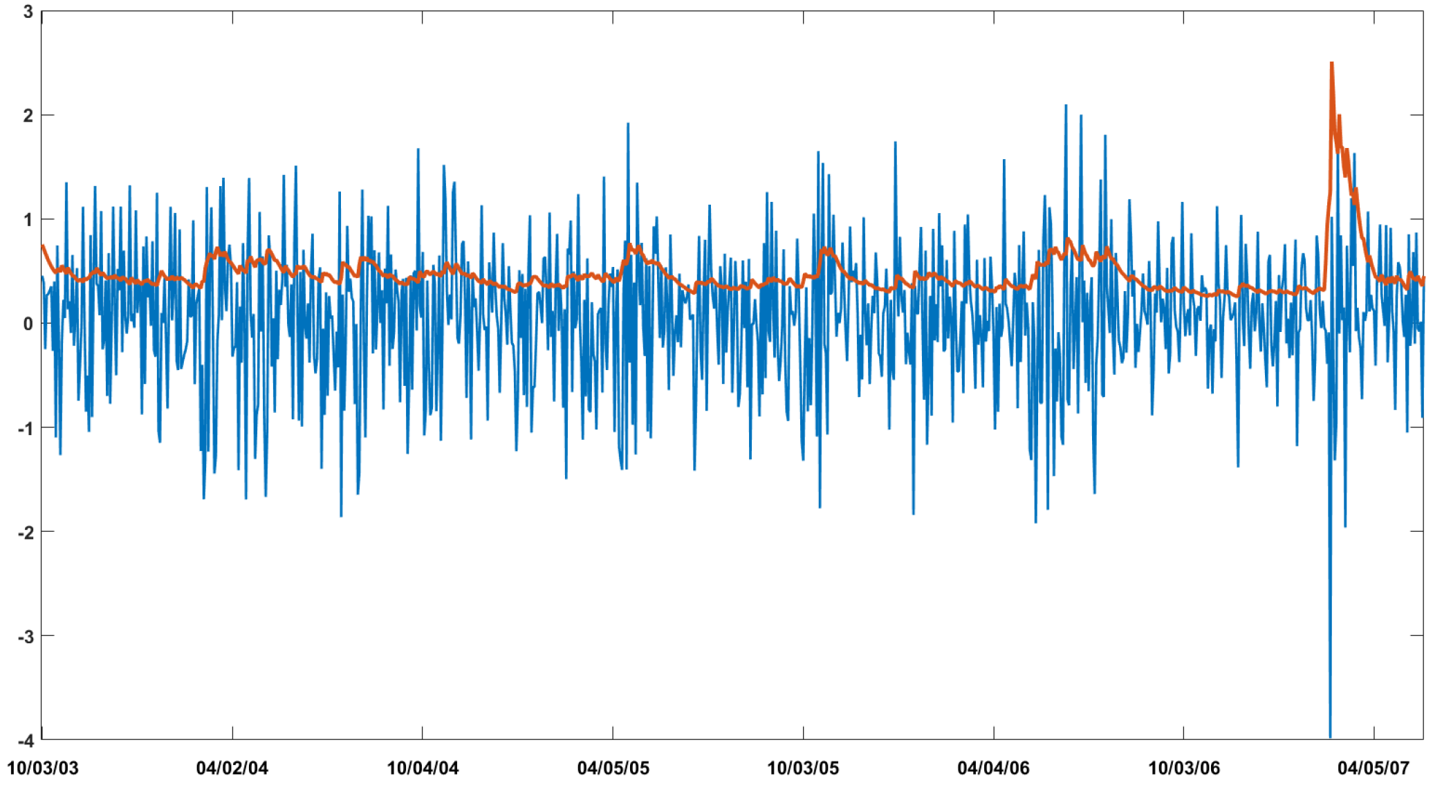
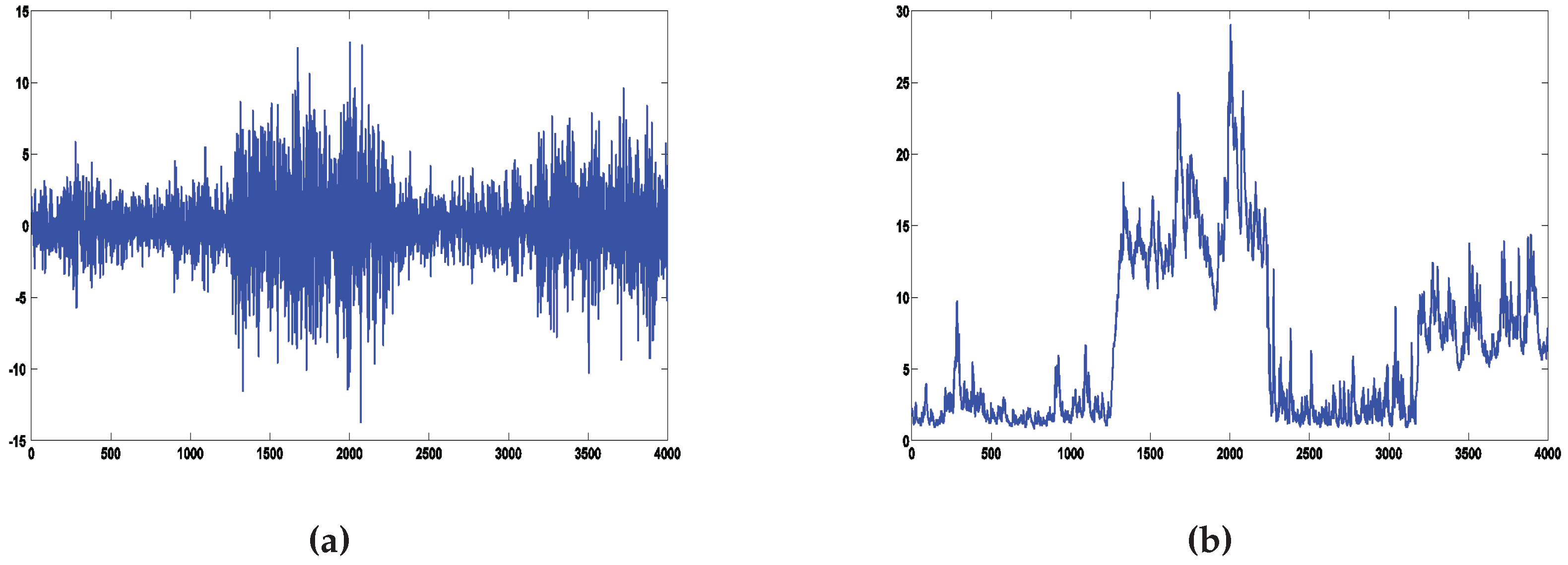
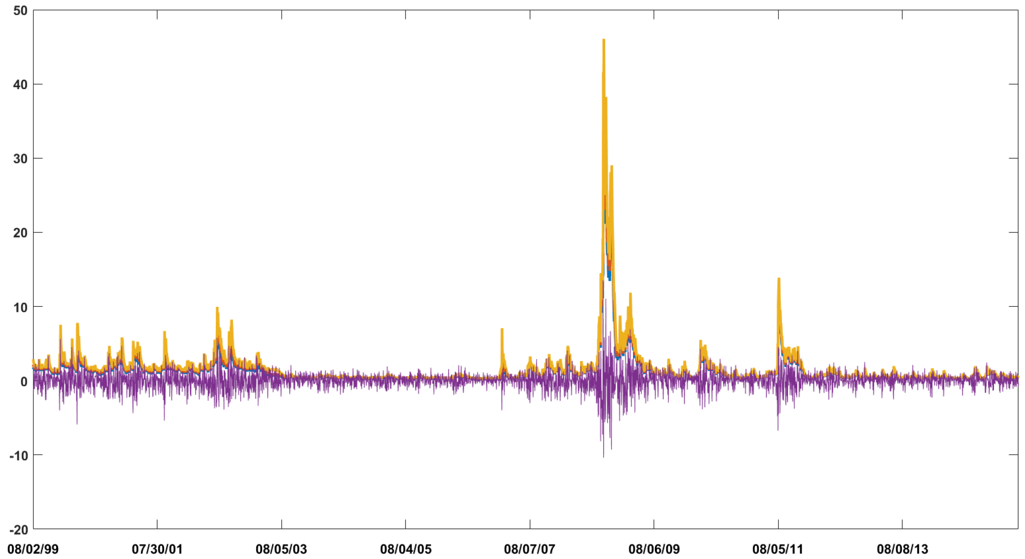
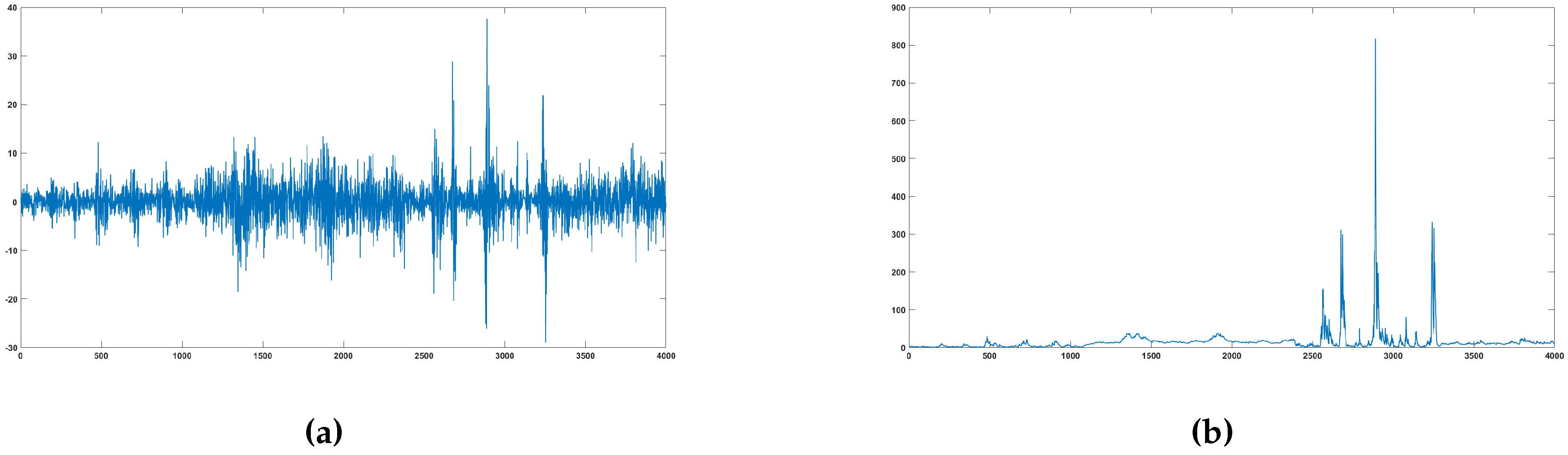
We generate 4000 observations from the data generating process (DGP) of

Table 4. Data generating process of the Change-point-Generalized Autoregressive Conditional Heteroskedastic (CP-GARCH) model.

	μ	ω	α	β	τ
Regime 1	0	0.1	0.1	0.85	1250
Regime 2	0	0.3	0.03	0.95	2230
Regime 3	0	0.25	0.2	0.70	3170
Regime 4	0	0.4	0.05	0.9	—

. The DGP exhibits four breaks in the volatility dynamic and tries to mimic the turbulent and quiet periods observed in a financial index. Figure 1 shows a simulated series and the corresponding volatility over time.

We use the marginal log-likelihood (MLL) for selecting the number of regimes by estimating several CP-GARCH models differing by their number of regimes (see [36]). As the TNT algorithm is both an off-line and an on-line method, we start by estimating the posterior distribution with 3000 observations (i.e., $\tau =3000$) and then we add one by one the remaining observations. For each model, we obtain 1001 estimated posterior distributions (from $\pi (x_{\tau }|y_{1:\tau })$ to $\pi (x_T|y_{1:T})$) and their respective 1001 MLLs. By so doing, the evolution of the best model over time can be observed. A sharp decrease in the MLL value means that the model cannot easily capture the new observation. According to the DGP Table 4, the model exhibiting three regimes should at least dominate over the first 170 observations and then the model with four regimes should gradually take the lead.

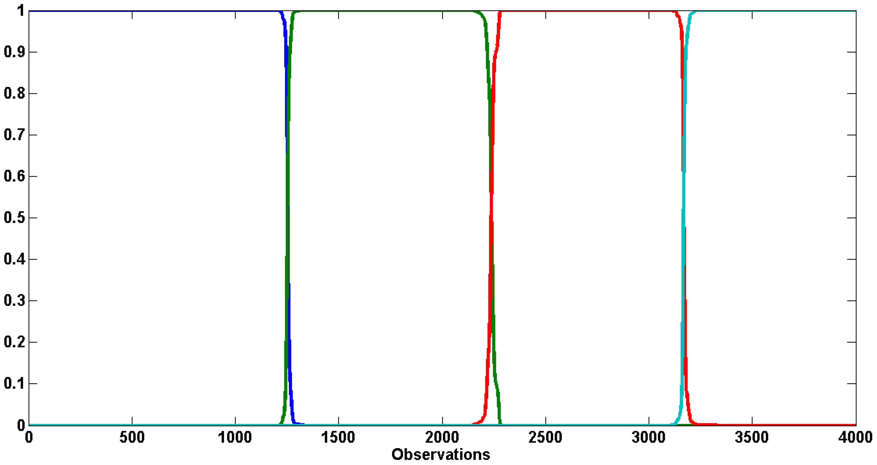
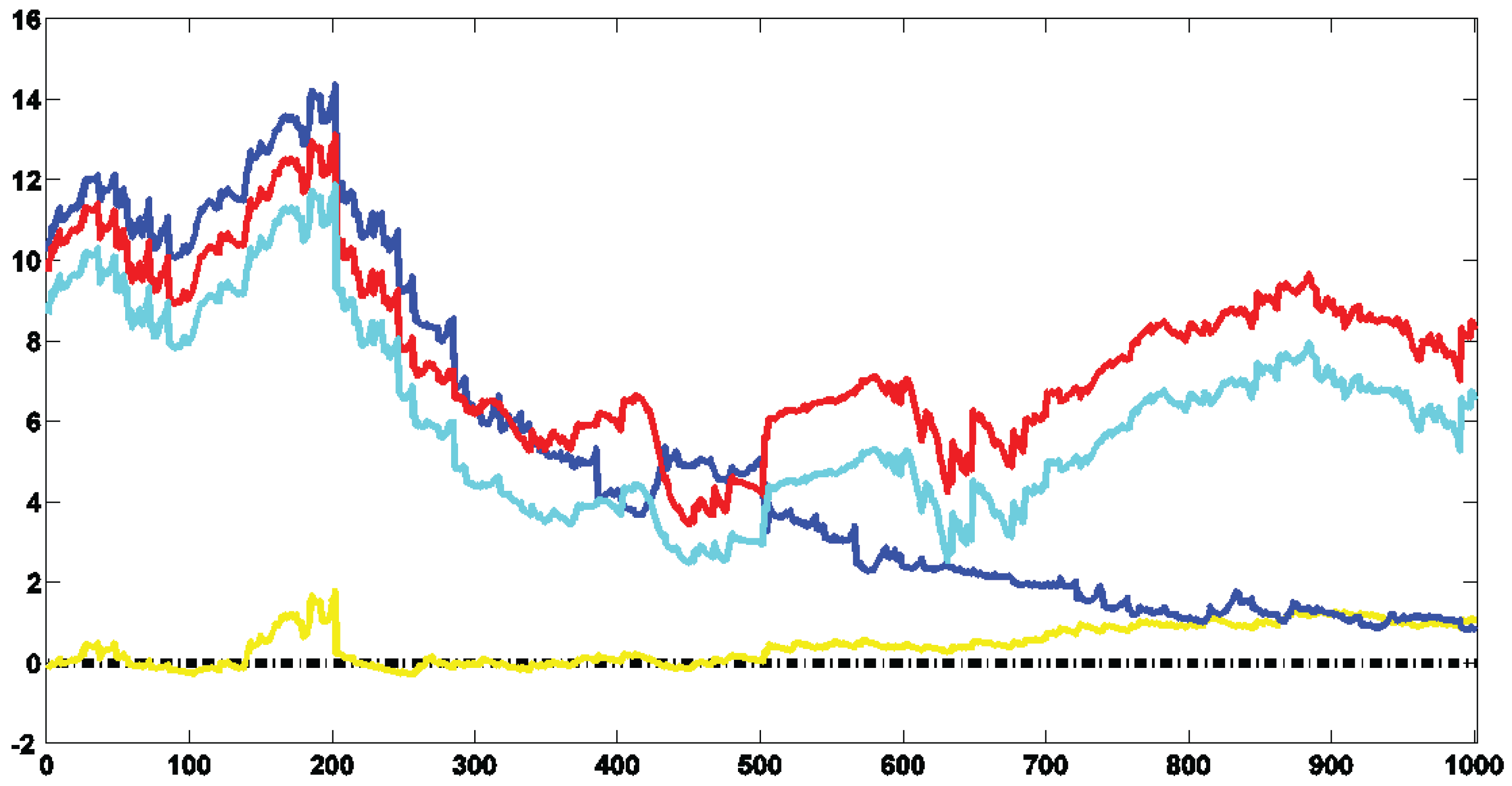
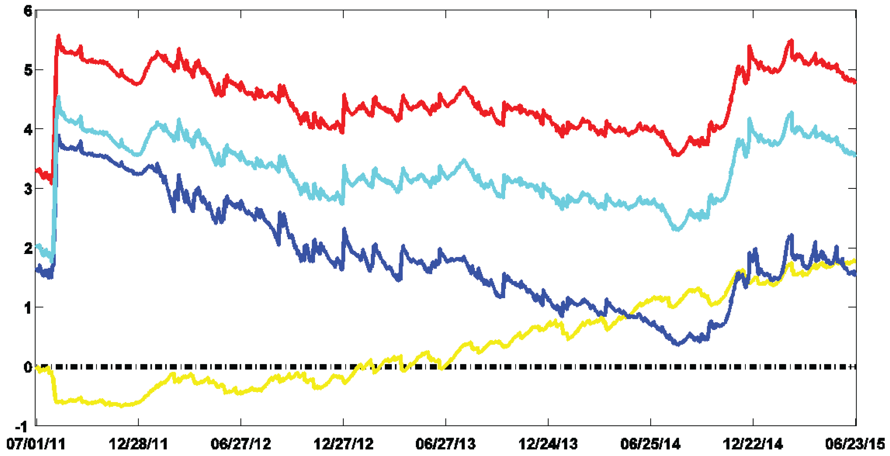
Figure 2 shows the log-Bayes factors (log-BFs) of CP-GARCH models with respect to the standard GARCH process (i.e., $K=1$).9 The best model over give or take the first 300 observations is the one exhibiting three regimes. Afterward, it is gradually dominated by the process with four regimes (in red). The on-line algorithm has been able to detect the coming break and according to the MLLs, around 150 observations are needed to identify it.

Table 5. Posterior means of the parameters of the CP-GARCH model with four regimes and their corresponding standard deviations.

	μ	ω	α	β	τ
Regime 1	–0.02	0.11	0.11	0.85	1253.7
	(0.04)	(0.04)	(0.03)	(0.04)	(9.91)
Regime 2	0.15	0.67	0.05	0.91	2238.4
	(0.13)	(0.21)	(0.02)	(0.03)	(17.42)
Regime 3	0.01	0.25	0.16	0.73	3169.4
	(0.04)	(0.08)	(0.03)	(0.05)	(11.33)
Regime 4	0.06	0.61	0.07	0.85
	(0.1)	(0.22)	(0.02)	(0.04)

documents the posterior means of the parameters of the model exhibiting the highest MLL at the end of the simulation (i.e., with a number of regimes equal to 4) as well as their standard deviations. We observe that the values are close to the true ones which indicates an accurate estimation of the model. The breaks are also precisely inferred. At least for this particular DGP, the TNT algorithm is able to draw the posterior distribution of the CP-GARCH models and correctly updates the distribution in the light of new observations.

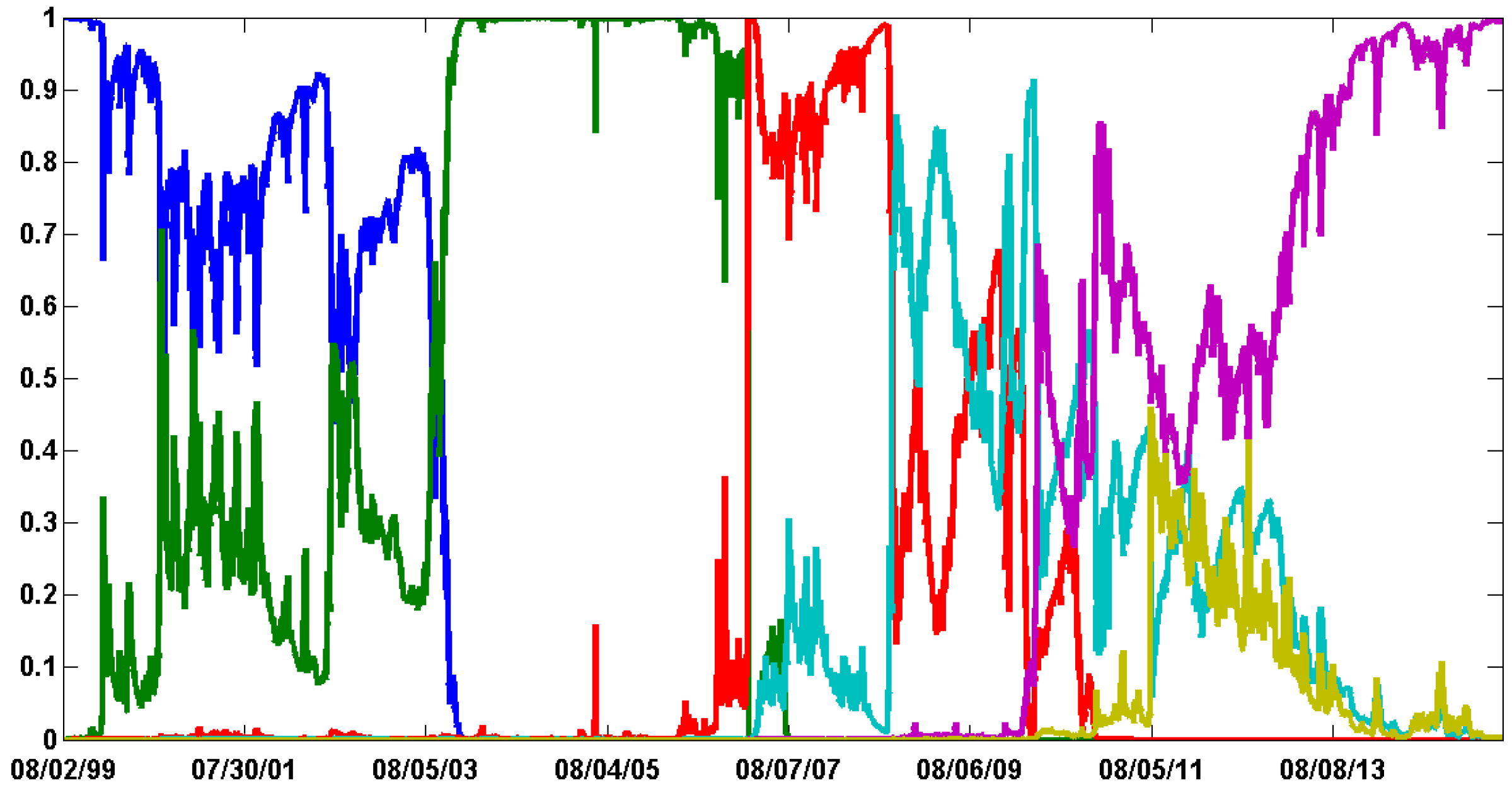
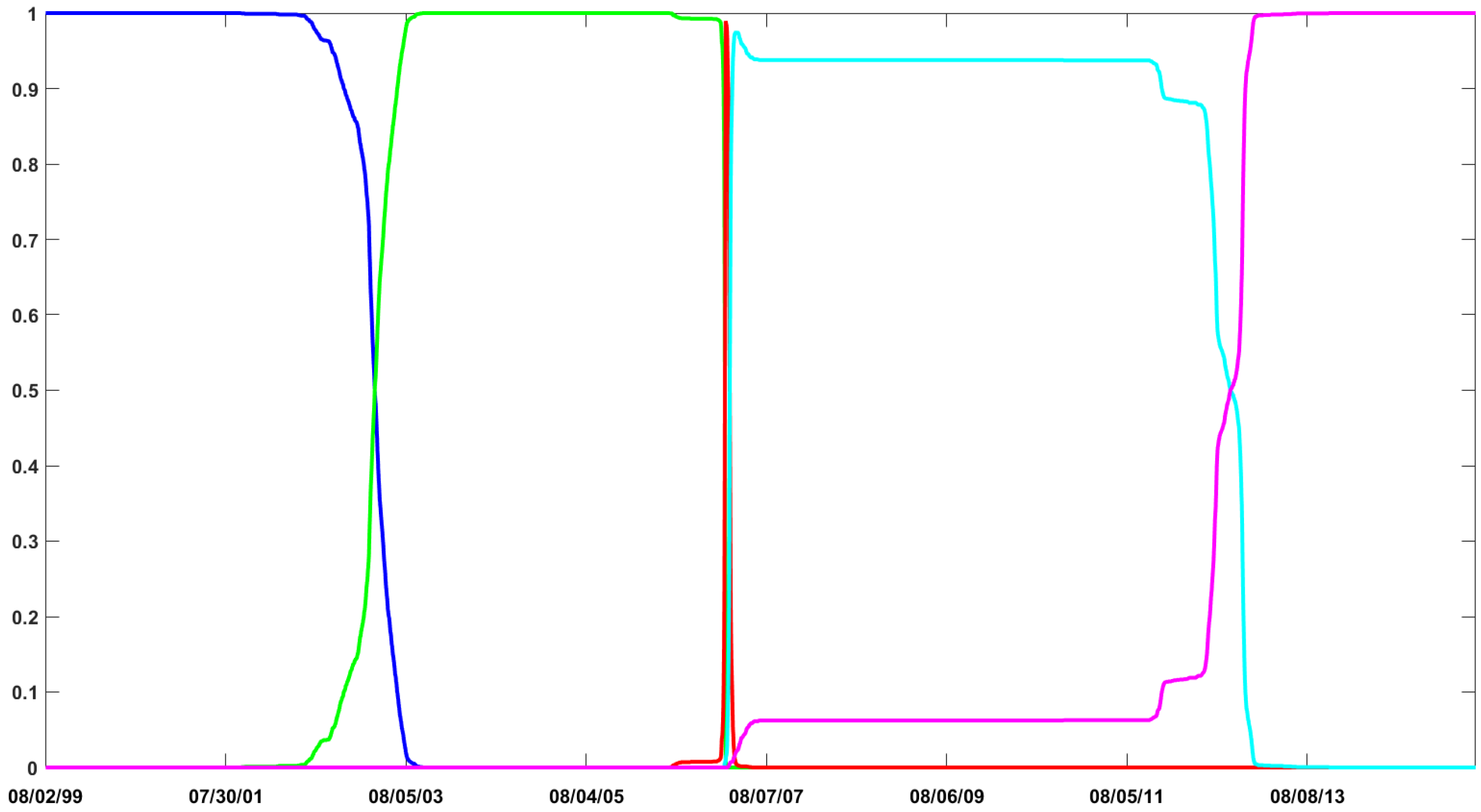
Eventually, one can have a look to the varying probabilities associated with each evolutionary update function. These probabilities are computed at each SMC iteration and are proportional to the Mahalanobis distances of the accepted draws.

Table 6. Probabilities (proportional to the Mahalabonis distance) of choosing a specific type of Metropolis-Hastings move. Mean stands for the average over the SMC iterations.

SMC Iteration	Stretch Move				Walk Move				DREAM Move
	Trigo	DE	Firefly	Standard	Trigo	DE	Firefly	Standard	Trigo	Standard
1th	0.1	0.1	0.1	0.1	0.1	0.1	0.1	0.1	0.1	0.1
10th	0.13	0.09	0.08	0.07	0.10	0.06	0.07	0.08	0.22	0.11
100th	0.14	0.11	0.13	0.13	0.11	0.04	0.06	0.16	0.09	0.04
last	0.11	0.12	0.11	0.11	0.08	0.05	0.06	0.10	0.17	0.09
Mean	0.13	0.12	0.12	0.11	0.10	0.05	0.06	0.14	0.12	0.06

documents the values for several SMC iterations. We observe that the probabilities highly vary over the SMC iterations. Moreover, the stretch move and the DREAM algorithm slightly dominate the walk update.

5. Empirical Application

As emphasized in the simulated exercise, the TNT algorithm allows to compare complex models through the marginal likelihoods. We examine the performances of the CP-GARCH models over time on the S&P 500 daily percentage returns spanning from February 08, 1999 to June 24, 2015 (4000 observations). We estimate the models with a number of regimes varying from 1 to 5 using the TNT algorithm and we fix the value $\tau =3000$ which controls the change from the tempered to the time domain.

To begin with,

Table 7. S&P 500 daily log-returns—marginal log-likelihoods (MLLs) of the CP-GARCH models given different number of regimes. The highest value is bolded.

#Regimes	1	2	3	4	5
MLL	–5732.6	–5730.86	–5731.1	–5727.87	–5729.1

documents the MLLs of the CP-GARCH models with different number of regimes when all the observations have been included. The best model exhibits four regimes.

Table 8. S&P 500 daily log-returns - posterior means of the parameters of the CP-GARCH model with four regimes and their corresponding standard deviations.

	μ	ω	α	β	τ
Regime 1	–0.01	0.16	0.11	0.81	25 March 2003
	(0.05)	(0.06)	(0.03)	(0.05)	(74.22)
Regime 2	0.06	0.02	0.05	0.91	14 February 2007
	(0.02)	(0.03)	(0.02)	(0.05)	(62.33)
Regime 3	–0.33	0.66	0.13	0.52	09 March 2007
	(0.34)	(0.22)	(0.15)	(0.20)	(32.63)
Regime 4	0.08	0.02	0.12	0.86
	(0.02)	(0.01)	(0.01)	(0.01)

provides the posterior means and the standard deviations of the best CP-GARCH model. Not surprisingly, the break dates occur after the dot-com bubble and at the beginning of the financial crisis. To link the results with the crisis event, Freddie Mac company announced that it will no longer buy the most risky subprime mortgages and mortgage-related securities in 17 February 2007. This date sometimes refers to the beginning of the collapse of the financial system.

We now turn to the recursive estimations of the CP-GARCH models. For the 1001 estimated posterior distributions (from $\pi (x_{\tau }|y_{1:\tau })$ to $\pi (x_T|y_{1:T})$), Figure 3 shows the log-BFs of the CP-GARCH models with respect to the fixed parameter GARCH model (i.e., $K=1$). The CP-GARCH model with four regimes dominates over the entire period. The process with five regimes fits similarly the data but is over-parametrized compared to the same model with four regimes. The difference between the two models comes from the penalization of this over-parametrization through the prior distributions. For interested readers, Appendix B provides additional results on the CP-GARCH models such as the filtered volatility of the preferred process and a detailed comparison with other CP-GARCH models exhibiting breaks in the intercept ω or with student innovations.

To end this study,

Table 9. S&P 500 daily log-returns—probabilities (proportional to the Mahalabonis distance) of choosing a specific type of Metropolis-Hastings move. Mean stands for the average over all the Sequential Monte Carlo (SMC) iterations. The highest probability is bolded.

SMC Iteration	Stretch Move				Walk Move				DREAM Move
	Trigo	DE	Firefly	Standard	Trigo	DE	Firefly	Standard	Trigo	Standard
1th	0.1	0.1	0.1	0.1	0.1	0.1	0.1	0.1	0.1	0.1
10th	0.12	0.09	0.08	0.06	0.10	0.06	0.07	0.07	0.24	0.12
100th	0.13	0.13	0.12	0.12	0.08	0.05	0.05	0.11	0.15	0.07
last	0.12	0.12	0.12	0.11	0.08	0.05	0.06	0.10	0.17	0.09
Mean	0.12	0.12	0.11	0.11	0.09	0.05	0.05	0.10	0.16	0.08

delivers the probabilities associated with each evolutionary update function for several SMC iterations. As in the simulated exercise, the stretch move and the DREAM algorithm slightly dominate the walk one. We also observe that the trigonometric move exhibits good mixing properties since its associated probabilities are high, especially for the DREAM-type update.

6. Conclusions

We develop an off-line and on-line SMC algorithm (called TNT) well-suited for situations where a relevant number of similar distributions has to be estimated. The method encompasses the off-line AIS of [5], the on-line IBIS algorithm of [6] and the RM method of [7] that all arise as special cases in the SMC sampler theory (see [8]). The TNT algorithm benefits from the conjugacy of the tempered and the time domains to avoid particle degeneracies observed in the on-line methods. More importantly, we introduce a new adaptive MCMC kernel based on the evolutionary optimization literature which consists in 10 different moves based on the interactions of the particles. These MCMC updates are selected according to some probabilities that are adjusted over the SMC iterations. Furthermore, the scale parameter of these updates are also automated thanks to the method of [31]. It makes the TNT algorithm fully generic and one needs only to plug the likelihood function, the prior distributions and the number of particles to use it.

The TNT sampler combines on-line and off-line estimations and is consequently suited for comparing complex models. Through a simulated exercise, the paper highlights that the algorithm is able to detect structural breaks of a CP-GARCH model on the fly. Eventually, an empirical application on the S&P 500 daily percentage log-returns shows that no break in the volatility of the GARCH model had arisen from 7 January 2011 to 24 June 2015. In fact, the MLL clearly indicates evidence in favor of a CP-GARCH model exhibiting four regimes in which the breaks occur at the end of the dot-com bubble as well as at the beginning of the financial crisis.

We believe that the TNT algorithm could be adapted to recent SMC algorithms such as [12,13] since they propose advanced SMC samplers based on the IBIS and the E-AIS samplers. Another avenue of research could be an application on change-point stochastic volatility models. Indeed, the evolutionary MCMC kernel is potentially able to update the volatility parameters of these models without filtering them.

References

1. J. Geweke. “Bayesian Inference in Econometric Models Using Monte Carlo Integration.” Econometrica 57 (1989): 1317–1339. [Google Scholar] [CrossRef]
2. A.F.M. Smith, and A.E. Gelfand. “Bayesian Statistics without Tears: A Sampling-Resampling Perspective.” Am. Stat. 46 (1992): 84–88. [Google Scholar]
3. N. Gordon, D. Salmond, and A.F.M. Smith. “Novel approach to nonlinear/non-Gaussian Bayesian state estimation.” IEE Proc. F Radar Signal Process. 140 (1993): 107–113. [Google Scholar] [CrossRef]
4. S. Chib, F. Nardari, and N. Shephard. “Markov chain Monte Carlo methods for stochastic volatility models.” J. Econom. 108 (2002): 281–316. [Google Scholar] [CrossRef]
5. R.M. Neal. “Annealed Importance Sampling.” Stat. Comput. 11 (1998): 125–139. [Google Scholar] [CrossRef]
6. N. Chopin. “A Sequential Particle Filter Method for Static Models.” Biometrika 89 (2002): 539–551. [Google Scholar] [CrossRef]
7. W.R. Gilks, and C. Berzuini. “Following a moving target—Monte Carlo inference for dynamic Bayesian models.” J. R. Stat. Soc. B 63 (2001): 127–146. [Google Scholar] [CrossRef]
8. P. Del Moral, A. Doucet, and A. Jasra. “Sequential Monte Carlo samplers.” J. R. Stat. Soc. B 68 (2006): 411–436. [Google Scholar] [CrossRef]
9. A. Jasra, D.A. Stephens, and C.C. Holmes. “On population-based simulation for static inference.” Stat. Comput. 17 (2007): 263–279. [Google Scholar] [CrossRef]
10. A. Jasra, D.A. Stephens, A. Doucet, and T. Tsagaris. “Inference for Lévy-Driven Stochastic Volatility Models via Adaptive Sequential Monte Carlo.” Scand. J. Stat. 38 (2011): 1–22. [Google Scholar] [CrossRef]
11. E. Jeremiah, S. Sisson, L. Marshall, R. Mehrotra, and A. Sharma. “Bayesian calibration and uncertainty analysis of hydrological models: A comparison of adaptive Metropolis and sequential Monte Carlo samplers.” Water Resour. Res. 47 (2011). [Google Scholar] [CrossRef]
12. P. Fearnhead, and B. Taylor. “An adaptive Sequential Monte Carlo Sampler.” Bayesian Anal. 8 (2013): 411–438. [Google Scholar] [CrossRef]
13. A. Fulop, and J. Li. “Efficient learning via simulation: A marginalized resample-move approach.” J. Econom. 176 (2013): 146–161. [Google Scholar] [CrossRef]
14. N. Chopin, P.E. Jacob, and O. Papaspiliopoulos. “SMC2: An efficient algorithm for sequential analysis of state space models.” J. R. Stat. Soc. B 75 (2013): 397–426. [Google Scholar] [CrossRef]
15. G. Durham, and J. Geweke. “Adaptive Sequential Posterior Simulators for Massively Parallel Computing Environments.” In Bayesian Model Comparison (Advances in Econometrics). Edited by I. Jeliazkov and D.J. Poirier. Bingley, UK: Emerald Group Publishing Limited, 2014, Volume 34, pp. 1–44. [Google Scholar]
16. E. Herbst, and F. Schorfheide. “Sequential Monte Carlo Sampling for DSGE Models.” J. Appl. Econom. 29 (2014): 1073–1098. [Google Scholar] [CrossRef]
17. L. Bauwens, A. Dufays, and J. Rombouts. “Marginal Likelihood for Markov Switching and Change-point GARCH Models.” J. Econom. 178 (2013): 508–522. [Google Scholar] [CrossRef]
18. J.A. Vrugt, C.J.F. ter Braak, C.G.H. Diks, B.A. Robinson, J.M. Hyman, and D. Higdon. “Accelerating Markov Chain Monte Carlo Simulation by Differential Evolution with Self-Adaptative Randomized Subspace Sampling.” Int. J. Nonlinear Sci. Numer. Simul. 10 (2009): 271–288. [Google Scholar] [CrossRef]
19. J.A. Christen, and C. Fox. “A general purpose sampling algorithm for continuous distributions (the t-walk).” Bayesian Anal. 5 (2010): 263–281. [Google Scholar] [CrossRef]
20. D. Foreman-Mackey, D.W. Hogg, D. Lang, and J. Goodman. “Emcee: The MCMC Hammer.” PASP 125 (2013): 306–312. [Google Scholar] [CrossRef]
21. P. Del Moral, A. Doucet, and A. Jasra. “On adaptive resampling strategies for sequential Monte Carlo methods.” Bernoulli 18 (2012): 252–278. [Google Scholar] [CrossRef]
22. A. Beskos, A. Jasra, and A. Thiery. “On the Convergence of Adaptive Sequential Monte Carlo Methods.” 2013. Available online: http://arxiv.org/pdf/1306.6462v2.pdf (accessed on 16th February 2016).
23. S. Das, and P. Suganthan. “Differential Evolution: A Survey of the State-of-the-Art.” IEEE Trans Evolut. Comput. 15 (2011): 4–31. [Google Scholar] [CrossRef]
24. R. Storn, and K. Price. “Differential Evolution—A Simple and Efficient Heuristic for Global Optimization over Continuous Spaces.” J. Glob. Optimiz. 11 (1997): 341–359. [Google Scholar] [CrossRef]
25. G.O. Roberts, and J.S. Rosenthal. “Optimal scaling for various Metropolis-Hastings algorithms.” Stat. Sci. 16 (2001): 351–367. [Google Scholar] [CrossRef]
26. S. Dutta, and S. Bhattacharya. “Markov chain Monte Carlo based on deterministic transformations.” Stat. Methodol. 16 (2014): 100–116. [Google Scholar] [CrossRef]
27. H.-Y. Fan, and J. Lampinen. “A Trigonometric Mutation Operation to Differential Evolution.” J. Glob. Optim. 27 (2003): 105–129. [Google Scholar] [CrossRef]
28. X.-S. Yang. “Firefly Algorithms for Multimodal Optimization.” In Stochastic Algorithms: Foundations and Applications. Edited by O. Watanabe and T. Zeugmann. Berlin, Germany: Springer, 2009, pp. 169–178. [Google Scholar]
29. C.J. Geyer. “Practical Markov Chain Monte Carlo.” Stat. Sci. 7 (1992): 473–511. [Google Scholar] [CrossRef]
30. J. Geweke. Contemporary Bayesian Econometrics and Statistics. Wiley Series in Probability and Statistics; Hoboken, NJ, USA: John Wiley and Sons, Inc., 2005. [Google Scholar]
31. Y. Atchadé, and J. Rosenthal. “On adaptive Markov chain Monte Carlo algorithms.” Bernoulli 11 (2005): 815–828. [Google Scholar] [CrossRef]
32. L.R. Rabiner. “A tutorial on hidden Markov models and selected applications in speech recognition.” Proc. IEEE 77 (1989): 257–286. [Google Scholar] [CrossRef]
33. R.E. Kalman. “A New Approach to Linear Filtering and Prediction Problems.” Trans. ASME J. Basic Eng. 82 (1960): 35–45. [Google Scholar] [CrossRef]
34. C. Andrieu, A. Doucet, and R. Holenstein. “Particle Markov Chain Monte Carlo Methods.” J. R. Stat. Soc. B 72 (2010): 269–342. [Google Scholar] [CrossRef]
35. Z. He, and J. Maheu. “Real Time Detection of Structural Breaks in GARCH Models.” Comput. Stat. Data Anal. 54 (2010): 2628–2640. [Google Scholar] [CrossRef]
36. S. Chib. “Estimation and comparison of multiple change-point models.” J. Econom. 86 (1998): 221–241. [Google Scholar] [CrossRef]
37. R. Kass, and A. Raftery. “Bayes Factors.” J. Am. Stat. Assoc. 90 (1995): 773–795. [Google Scholar] [CrossRef]
38. L. Bauwens, A. Dufays, and B. De Backer. “Estimating and forecasting structural breaks in financial time series.” J. Empir. Financ., 2011. [Google Scholar] [CrossRef]
39. J. Liu, and M. West. “Combined Parameter and State Estimation in Simulation-Based Filtering.” In Sequential Monte Carlo Methods in Practice. Edited by A. Doucet, N. de Freitas and N. Gordon. New York, USA: Springer, 2001, pp. 197–224. [Google Scholar]
40. M.K. Pitt, and N. Shephard. “Filtering via Simulation: Auxiliary Particle Filters.” J. Am. Stat. Assoc. 94 (1999): 590–599. [Google Scholar] [CrossRef]
41. S. Ko, T. Chong, and P. Ghosh. “Dirichlet Process Hidden Markov Multiple Change-point Model.” Bayesian Anal. 2 (2015): 275–296. [Google Scholar] [CrossRef]
42. J. Carpenter, P. Clifford, and P. Fearnhead. “Improved particle filter for nonlinear problems.” IEE Proc. Radar Sonar Navig. 146 (1999): 2–7. [Google Scholar] [CrossRef]
• 1.whereas the sequence does not have to necessarily evolve over the time domain
• 2.enhanced in the sense that the AIS incorporates a re-sampling step
• 3.The IBIS algorithm being a particular case
• 4.Theorem 1 in [6] ensures that with a sufficiently large number of particles M, any relative precision of the importance sampling can be obtained if the number of observations already covered is large enough in the IBIS context
• 5.a piecewise cooling linear function for [8] and a quadratic function for [16]
• 6.in the sense of M
• 7.The best particle is replaced by an average over the particles g = 1 δ x t r 1 ( g ) δ which further diversifies the proposed parameters.
• 8.Although only the chosen mixture enters in the MH acceptance ratio, the MCMC algorithm is still valid. For further explanations, see [30], section Transition Mixtures.
• 9.We remind that the log-BF is computed as the difference of the MLL of two models. Following the informal rule of [37], if the logarithm of the Bayes factor exceeds 3, we have strong evidence in favor of the model with the highest value.
• 10.taking into account the degree of freedom of the student distribution.
• 11.To compare with the specification of the paper, we have included the mean parameters { μ i } i = 1 K .
Figure 1. Simulated series from the data generating process (DGP) exhibited in Table 4 and its corresponding volatility over time. (a) Simulated series; (b) Volatility over time.
Econometrics 04 00012 g001
Figure 2. Log-BF over time of the CP-GARCH models in relation to the GARCH one. The log-BF of the CP-GARCH model with two, three, four and five regimes are depicted in yellow, blue, red and cyan respectively. A positive value provides evidence in favor of the considered model compared to the GARCH one.
Econometrics 04 00012 g002
Figure 3. S&P 500 daily log-returns — log-BFs over time of the volatility models in relation to the GARCH one. The log-BFs of the CP-GARCH models with two, three, four and five regimes are depicted in yellow, blue, red and cyan respectively. A positive value provides evidence in favor of the considered model compared to the GARCH one.
Econometrics 04 00012 g003
Figure B1. S&P 500 daily log-returns in relation with the 5% (blue), 50% (red) and the 95% (yellow) quantiles of the filtered volatility posterior distribution provided by the CP-GARCH model with 4 regimes.
Econometrics 04 00012 g004
Figure B2. S&P 500 daily log-returns over the quiet period preceding the financial crisis in relation with the median of the filtered volatility posterior distribution provided by the CP-GARCH model with four regimes.
Econometrics 04 00012 g005
Figure B3. Simulated series from the DGP Table B5 and its corresponding volatility over time. (a) Simulated series; (b) Volatility over time.
Econometrics 04 00012 g006
Figure C1. Simulated series—filtered probabilities of the states given by the He and Maheu’s algorithm. The probabilities of the first state are displayed in blue, the second in green, the third in red and the last three regimes have virtually zero probabilities over the entire sample.
Econometrics 04 00012 g007
Figure C2. Simulated series—smooth probabilities of the states given by the TNT algorithm. The probabilities of the first state are displayed in blue, the second in green, the third in red and the last one in turquoise.
Econometrics 04 00012 g008
Figure C3. S&P 500 daily log-returns—filtered probabilities of the states given by the He and Maheu’s algorithm. The probabilities of the first state are given in blue, the second in green, the third in red and the fourth in turquoise, the fifth in purple and the last one in pale green.
Econometrics 04 00012 g009
Figure C4. S&P 500 daily log-returns - smooth probabilities of the states given by the TNT algorithm for the CP-GARCH model exhibiting five regimes. The probabilities of the first state are displayed in blue, the second in green, the third in red, the fourth in turquoise and the fifth in purple.
Econometrics 04 00012 g010