Testing in a Random Effects Panel Data Model with Spatially Correlated Error Components and Spatially Lagged Dependent Variables

Abstract

We propose a random effects panel data model with both spatially correlated error components and spatially lagged dependent variables. We focus on diagnostic testing procedures and derive Lagrange multiplier (LM) test statistics for a variety of hypotheses within this model. We first construct the joint LM test for both the individual random effects and the two spatial effects (spatial error correlation and spatial lag dependence). We then provide LM tests for the individual random effects and for the two spatial effects separately. In addition, in order to guard against local model misspecification, we derive locally adjusted (robust) LM tests based on the Bera and Yoon principle (Bera and Yoon, 1993). We conduct a small Monte Carlo simulation to show the good finite sample performances of these LM test statistics and revisit the cigarette demand example in Baltagi and Levin (1992) to illustrate our testing procedures.

1. Introduction

Spatial econometric models have been extensively used to study regional effects and interdependence between different spatial units. Most of the widely used spatial models are variants of the benchmark models developed in Cliff and Ord (1973, 1981) [1,2] and Anselin (1988a) [3]. Based on the form of spatially correlated error components and/or spatially lagged dependent variables, these models better fit the real world data generating process by explicitly considering the spatial interdependence. Hypothesis testing for spatial dependence has been developed rapidly in the recent literature. For standard LM tests of spatial dependence in cross section models, see Anselin (1988a, b) [3,4], Anselin and Bera (1998) [5], and Anselin (2001) [6]. For standard LM tests of spatial dependence in panel data models, Baltagi et al., (2003) [7] provide tests for random effects and/or spatial error correlation. Baltagi and Liu (2008) [8] provide tests for random effects and/or spatial lag dependence. Debarsy and Ertur (2010) [9] derive tests in the spatial panel data model with individual fixed effects based on Lee and Yu (2010) [10]. Qu and Lee (2012) [11] consider tests in spatial models with limited dependent variables. Baltagi et al., (2013) [12] extend the model in Kapoor et al., (2007) [13] by allowing for different spatial correlation parameters in the individual random effects and in the disturbances, and they derive the corresponding LM tests. Further, standardized versions of the LM tests are discussed in Yang (2010) [14], Baltagi and Yang (2013a) [15] to remedy distributional misspecifications in finite sample and sensitivity to spatial layout. Born and Breitung (2011) [16], Baltagi and Yang (2013b) [17] discuss versions of LM tests that are robust against unknown heteroskedasticity. Recently, Yang (2015) [18] provides residual-based bootstrap procedure to obtain improved approximations to the finite sample critical values of the LM test statistics in spatial econometric models.

However, to the best of our knowledge, there are no test statistics treating the individual random effects, the spatial error correlation, and the spatial lag dependence simultaneously. We contribute to the literature by constructing various LM test statistics in such a general framework, or the so-called spatial autoregressive model with autoregressive disturbances (SARAR). Our results are useful for applied researchers to implement and perform model diagnostic testing in the SARAR framework. In particular, we first derive the joint LM test for the individual random effects and the two spatial effects. We next derive LM tests for the individual random effects. Finally, we derive LM tests for the two spatial effects. In addition, we provide robust LM tests in some cases as needed in order to guard against local misspecification. We emphasize some key features of the robust LM test in the following.

Bera and Yoon (1993) [19] argue that the LM test with specific values of the nuisance parameters (marginal LM test) might suffer from local misspecification in the nuisance parameters. They propose robust LM test to guard against such local misspecification, see also Anselin et al., (1996) [20], Bera et al., (2001, 2009, 2010) [21,22,23], and He and Lin (2013) [24]. Here, we emphasize two advantages of the robust LM test. First, the asymptotic size of marginal LM test will be distorted under local misspecification in the nuisance parameters since it follows a non-central ${\chi }^2$ distribution. On the other hand, robust LM test follows a ${\chi }^2$ distribution under such misspecification, thus it can provide valid asymptotic size as long as the misspecification is local. Second, while LM test without specifying values of the nuisance parameters (conditional LM test) does not suffer from such size distortion, it generally needs the maximum likelihood estimator (MLE), which could be costly in computation. In contrast, the robust LM test only requires restricted estimator under the relevant joint null hypothesis, which is simply the ordinary least square (OLS) estimator in most cases. Therefore, the robust LM test can provide result as good as the conditional LM test at a lower computational cost, provided that the deviation of nuisance parameters is local. However, there is one potential loss in using the robust LM test. If the values of nuisance parameters are correctly specified, the robust LM test is in general less powerful than the marginal LM test. Also, when the nuisance parameters deviate far away from the pre-specified values, the robust LM test is generally invalid. In sum, the standard LM tests (marginal and conditional LM tests) and the robust LM tests complement each other, and they should be used together for inference purposes.

In this paper, we maintain the assumption of random effects model, while an alternative specification is the fixed effects model with spatial dependence as in Lee and Yu (2010) [10], Debarsy and Ertur (2010) [9], and He and Lin (2013) [24]. On the one hand, the random effects specification is a parsimonious way to allow for individual effects in different spatial units and it will be particularly useful for testing and selection in microeconometric applications when the number of units is very large. On the other hand, the fixed effects specification, which allows for correlation between the individual effects and the covariates, is more suited for many macro studies when the number of units is not very large (see Elhorst (2014) [25] for more discussion on comparison of the random effects model and the fixed effects model).

The rest of the paper is organized as follows. Model specification is discussed in Section 2. The LM test statistics are presented In Section 3. In Section 4, we report the Monte Carlo simulation results to show their satisfactory finite sample size and power performances. In Section 5, we provide an empirical example to illustrate our testing procedures. Section 6 concludes with suggestions for future research. All mathematical derivations are relegated to the Appendices.

2. The Model

Suppose that the data is generated according to the following spatial panel data model, for $t=1,2,···,T,$

$$\left\{\begin{array}{c}{y}_t=\lambda W{y}_t+X_t\beta +{ϵ}_t,\hfill \\ {ϵ}_t=\rho M{ϵ}_t+\mu +v_t.\hfill \end{array}\right.$$

(2.1)

In the above specification, $y_t={(y_{t1},y_{t2},···,y_{tN})}^{\prime }$ is an $N\times 1$ vector of dependent variable for period t. It is spatially interdependent, as reflected by the spatial lag dependence coefficient λ. $X_t$ is an $N\times (K+1)$ matrix of non-stochastic regressors for period t, with the first column to be ones, and $\beta ={({\beta }_0,{\beta }_1,···,{\beta }_K)}^{\prime }$ is the corresponding $(K+1)\times 1$ slope parameter vector. ${ϵ}_t={({ϵ}_{t1},{ϵ}_{t2},···,{ϵ}_{tN})}^{\prime }$ is an $N\times 1$ vector of the regression error term for period t. The error vector is also spatially correlated, as reflected by the spatial error correlation coefficient ρ. $\mu ={({\mu }_1,{\mu }_2,···,{\mu }_N)}^{\prime }$ is an $N\times 1$ vector representing the individual random effects. The random effects terms $\left\{{\mu }_i\right\},i=1,···,N$ are i.i.d. across i, with zero mean, variance ${\sigma }_{\mu }^2$ and $\text{E}|{\mu }_i{|}^{4+c_1}<\infty$ for some $c_1>0$. $v_t={(v_{t1},v_{t2},···,v_{tN})}^{\prime }$ is an $N\times 1$ vector of innovation terms. The innovation terms $\left\{v_{ti}\right\},t=1,···,T,i=1,···,N$ are i.i.d. across i and t, with zero mean, variance ${\sigma }_v^2$ and $\text{E}|v_{ti}{|}^{4+c_2}<\infty$ for some $c_2>0$ (see Lee and Yu (2012) [26] for other regularity and identification conditions as needed for asymptotic theory). W and M are nonstochastic spatial weights matrices of size $N\times N$. Typically, they are specified by the first-order rook contiguity criterion and are row-standardized so that each row sums up to one.

By stacking across t, the model can be written as

$$\left\{\begin{array}{c}y=\lambda (I_T\otimes W)y+X\beta +ϵ,\hfill \\ ϵ=\rho (I_T\otimes M)ϵ+{\iota }_T\otimes \mu +v,\hfill \end{array}\right.$$

(2.2)

where $y={(y_1^{\prime },y_2^{\prime },···,y_T^{\prime })}^{\prime },X={(X_1^{\prime },X_2^{\prime },···,X_T^{\prime })}^{\prime },ϵ={({ϵ}_1^{\prime },{ϵ}_2^{\prime },···,{ϵ}_T^{\prime })}^{\prime }$, and $v={(v_1^{\prime },v_2^{\prime },···,v_T^{\prime })}^{\prime }$. ${\iota }_T$ is a $T\times 1$ vector of ones, I denotes the identity matrix with its dimension in the subscript, and ⊗ denotes the kronecker product. Let $A=[I_T\otimes (I_N-\rho M)]$, and $B=[I_T\otimes (I_N-\lambda W)]$. The error component ϵ is expressed as $ϵ=A^{-1}({\iota }_T\otimes \mu +v)$, with $\text{E}\left[ϵ\right]=0$, $\text{Var}\left[ϵ\right]={\Omega }_{ϵ}=A^{-1}\Omega {\left(A^{-1}\right)}^{\prime }$, where $\Omega =[J_T\otimes \left({\sigma }_{\mu }^2{I}_N\right)+I_T\otimes \left({\sigma }_v^2{I}_N\right)]$. Using the results in Magnus (1982) [27], we get ${\Omega }^{-1}={(T{\sigma }_{\mu }^2+{\sigma }_v^2)}^{-1}\overline{J_T}\otimes I_N+{\left({\sigma }_v^2\right)}^{-1}{E}_T\otimes I_N$, and $|\Omega |={(T{\sigma }_{\mu }^2+{\sigma }_v^2)}^N{\left({\sigma }_v^2\right)}^{N(T-1)}$, where $\overline{J_T}=J_T/T$, $J_T={\iota }_T{\iota }_T^{\prime }$, $E_T=I_T-\overline{J_T}$. Notice that $y=B^{-1}X\beta +B^{-1}ϵ$, with $\text{E}\left[y\right]=B^{-1}X\beta$ and $\text{Var}\left[y\right]={\Omega }_y=B^{-1}{A}^{-1}\Omega {\left(A^{-1}\right)}^{\prime }{\left(B^{-1}\right)}^{\prime }$. We have ${\Omega }_y^{-1}=B^{\prime }{A}^{\prime }{\Omega }^{-1}AB$, and $|{\Omega }_y{|=|B|}^{-2}{\left|A\right|}^{-2}{(T{\sigma }_{\mu }^2+{\sigma }_v^2)}^N{\left({\sigma }_v^2\right)}^{N(T-1)}$.

Let $\delta ={({\beta }^{\prime },\rho ,\lambda ,{\sigma }_{\mu }^2,{\sigma }_v^2)}^{\prime }$ and $ϵ=By-X\beta$, the log-likelihood function of the random vector y as if it is normally distributed is

$$L\left(\delta \right)=-\frac{NT}{2}\text{ln}\left(2\pi \right)-\frac{N}{2}\text{ln}\left(T{\sigma }_{\mu }^2+{\sigma }_v^2\right)-\frac{N(T-1)}{2}\text{ln}\left({\sigma }_v^2\right)+\text{ln}\left|A\right|+\text{ln}\left|B\right|-\frac{1}{2}{ϵ}^{\prime }{A}^{\prime }{\Omega }^{-1}Aϵ$$

(2.3)

3. LM and Robust LM Test Statistics

In this section, we provide explicit formulae for the LM test statistics. We first present the joint LM test for both the individual random effects and the spatial effects. We then provide LM test statistics for the individual random effects. Lastly, we present LM test statistics for the spatial effects, namely, the spatial error correlation and/or the spatial lag dependence.1 In addition, we provide formulae for robust LM tests when necessary.

Before presenting the LM test statistics, we introduce the following notations for easy reference. Let $R_1=M{(I_N-\rho M)}^{-1}$, $R_2=W{(I_N-\rho M)}^{-1}$, $R_3=W{(I_N-\lambda W)}^{-1}$, and $R_4=(I_N-\rho M^{\prime })(I_N-\rho M)$. Let ${\widehat{z}}_{\rho }={\widehat{ϵ}}^{\prime }{\widehat{A}}^{\prime }{\widehat{\Omega }}^{-1}(I_T\otimes M)\widehat{ϵ}$, ${\widehat{z}}_{\lambda }={\widehat{ϵ}}^{\prime }{\widehat{A}}^{\prime }{\widehat{\Omega }}^{-1}\widehat{A}(I_T\otimes W)y$, and ${\widehat{z}}_{{\sigma }_{\mu }^2}=\left[{\widehat{ϵ}}^{\prime }{\widehat{A}}^{\prime }({\overline{J}}_T\otimes I_N)\widehat{A}\widehat{ϵ}\right]/{\widehat{\sigma }}_v^2-N$, where $\widehat{ϵ}=\widehat{B}y-X\widehat{\beta }$, $\widehat{A}$, $\widehat{B}$, $\widehat{\Omega }$, $\widehat{\beta }$, and ${\widehat{\sigma }}_v^2$ are restricted MLEs of A, B, Ω, β, and ${\sigma }_v^2$ under the null hypotheses, respectively. Next, define $\widehat{\nu }={\widehat{y}}^{\prime }(I_T\otimes W^{\prime }){\widehat{A}}^{\prime }{\widehat{\Omega }}^{-1}\widehat{A}(I_T\otimes W)\widehat{y}$, $\widehat{\tau }=T^2(b_1{b}_3-b_2^2)+T{b}_1\widehat{\omega }$, where $\widehat{\omega }={\widehat{y}}^{\prime }(I_T\otimes W^{\prime }){\widehat{A}}^{\prime }[{\widehat{\Omega }}^{-1}-{\widehat{\Omega }}^{-1}\widehat{A}X{(X^{\prime }{\widehat{A}}^{\prime }{\widehat{\Omega }}^{-1}\widehat{A}X)}^{-1}{X}^{\prime }{\widehat{A}}^{\prime }{\widehat{\Omega }}^{-1}]\widehat{A}(I_T\otimes W)\widehat{y}$, $\widehat{y}={\widehat{B}}^{-1}X\widehat{\beta }$, $b_1=\text{tr}(M^{\prime }M+MM),b_2=\text{tr}(M^{\prime }W+MW),b_3=\text{tr}(W^{\prime }W+WW)$, and $\text{tr}(·)$ is the trace operator. Finally, let

$$\widehat{\xi }=\frac{NT{\widehat{\vartheta }}_2+N\widehat{\omega }-2T{\widehat{\vartheta }}_3^2}{T{b}_1(NT{\widehat{\vartheta }}_2+N\widehat{\omega }-2T{\widehat{\vartheta }}_3^2)-N{\left(T{\widehat{\vartheta }}_1\right)}^2},\widehat{\zeta }=\frac{N{\widehat{\theta }}_1-2{\widehat{\theta }}_3^2}{(N{\widehat{\theta }}_1-2{\widehat{\theta }}_3^2)(T{\widehat{\theta }}_4+\widehat{\omega })-NT{\widehat{\theta }}_2^2}$$

where ${\widehat{\vartheta }}_1=\text{tr}[(M+M^{\prime }){\widehat{R}}_3]$, ${\widehat{\vartheta }}_2=\text{tr}({\widehat{R}}_3{\widehat{R}}_3+{\widehat{R}}_3{\widehat{R}}_3^{\prime })$, ${\widehat{\vartheta }}_3=\text{tr}({\widehat{R}}_3)$, ${\widehat{\theta }}_1=\text{tr}\left({\widehat{R}}_1{\widehat{R}}_1+{\widehat{R}}_1{\widehat{R}}_1^{\prime }\right)$, ${\widehat{\theta }}_2=\text{tr}\left[W{\widehat{R}}_1+{\widehat{R}}_2{\widehat{R}}_1^{\prime }(I_N-\widehat{\rho }M)\right]$, ${\widehat{\theta }}_3=\text{tr}\left({\widehat{R}}_1\right)$, ${\widehat{\theta }}_4=\text{tr}\left(WW\right)+\text{tr}\left({\widehat{R}}_2{\widehat{R}}_2^{\prime }{\widehat{R}}_4\right)$, and ${\widehat{R}}_1,{\widehat{R}}_2,{\widehat{R}}_3,{\widehat{R}}_4$ are restricted MLEs of $R_1,R_2,R_3,R_4$, respectively.

3.1. Jointly Testing for Random Effects and Spatial Effects

Now we are ready to present the test statistics. We first construct the joint LM test statistic for the individual random effects and the spatial effects, namely, the spatial error correlation and the spatial lag dependence. The joint hypothesis is $H_0^a$: ${\sigma }_{\mu }^2=\rho =\lambda =0\mathit{\text{vs.}}$ $H_1^a$: at least one of ${\sigma }_{\mu }^2,\rho \text{and}\lambda$ is not zero. Thus we are testing the classical pooled panel data model against the full specification in (2.1), the LM test in this case is given by

$$L{M}_a=\frac{T{b}_3+{\widehat{\omega }}_a}{{\widehat{\tau }}_a}{\widehat{z}}_{\rho ,a}^2+\frac{T{b}_1}{{\widehat{\tau }}_a}{\widehat{z}}_{\lambda ,a}^2-\frac{2T{b}_2}{{\widehat{\tau }}_a}{\widehat{z}}_{\rho ,a}{\widehat{z}}_{\lambda ,a}+\frac{T}{2N(T-1)}{\widehat{z}}_{{\sigma }_{\mu }^2,a}^2,$$

(3.1)

where ${\widehat{\omega }}_a=[{\widehat{y}}_a^{\prime }(I_T\otimes W^{\prime })(I_{NT}-X{\left(X^{\prime }X\right)}^{-1}{X}^{\prime })(I_T\otimes W){\widehat{y}}_a]/{\widehat{\sigma }}_{v,a}^2$, ${\widehat{\sigma }}_{v,a}^2=\left({\widehat{ϵ}}_a^{\prime }{\widehat{ϵ}}_a\right)/\left(NT\right)$, ${\widehat{ϵ}}_a=y-{\widehat{y}}_a$, ${\widehat{y}}_a=X{\widehat{\beta }}_a$, ${\widehat{\tau }}_a=T^2(b_1{b}_3-b_2^2)+T{b}_1{\widehat{\omega }}_a$, ${\widehat{z}}_{\rho ,a}=\left[{\widehat{ϵ}}_a^{\prime }(I_T\otimes M){\widehat{ϵ}}_a\right]/{\widehat{\sigma }}_{v,a}^2$, ${\widehat{z}}_{\lambda ,a}=\left[{\widehat{ϵ}}_a^{\prime }(I_T\otimes W)y\right]/{\widehat{\sigma }}_{v,a}^2$, ${\widehat{z}}_{\mu ,a}=\left[{\widehat{ϵ}}_a^{\prime }({\overline{J}}_T\otimes I_N){\widehat{ϵ}}_a\right]/{\widehat{\sigma }}_{v,a}^2-N$, and ${\widehat{\beta }}_a$ is the OLS estimator of β. Under $H_0^a$, $L{M}_a$ is asymptotically distributed as ${\chi }_3^2$, where ${\chi }_d^2$ denotes the ${\chi }^2$ distribution with degree of freedom d.

The test statistic $L{M}_a$ is useful in practice, and it is simple to compute since only the OLS estimator is required. Researchers should first use this joint LM test to determine if there is individual random effects and/or spatial effects in the general specification (2.1). If the joint null hypothesis cannot be rejected, then it is reasonable to just adopt the classical pooled panel data model. Otherwise either the individual random effects, or the spatial error correlation, or the spatial lag dependence need to be considered. As in Baltagi et al., (2003) [7], we do not provide formal proofs for the asymptotic null distributions of the LM test statistics in this paper, but these distributions are likely to hold by using the Central Limit Theorems (CLTs) in Kelejian and Prucha (2001, 2010) [28,29] under similar sets of low level assumptions in their papers.

3.2. Testing for Random Effects

In this section, we focus on testing for the individual random effects in various spatial panel data models. We provide formulae for the standard LM tests as well as formulae for the robust LM tests when necessary. The first hypothesis we consider is $H_0^b$: ${\sigma }_{\mu }^2=0(\rho =\lambda =0)\mathit{\text{vs.}}$ $H_1^b$: ${\sigma }_{\mu }^2>0(\rho =\lambda =0)$. The null model is the classical pooled panel data model, and the alternative model is the random effects panel data model without spatial effects. The LM test denoted as $L{M}_b$, is available in Baltagi et al., (2003) [7]. Moreover, it can be shown that the robust LM test is the same as $L{M}_b$ in this case. We thus omit these formulae for the sake of compactness.

The second hypothesis is $H_0^c$: ${\sigma }_{\mu }^2=0(\rho \ne 0,\lambda =0)\mathit{\text{vs.}}$ $H_1^c$: ${\sigma }_{\mu }^2>0(\rho \ne 0,\lambda =0)$.2 Under the null hypothesis, it is the pooled panel data model with spatial error correlation. Under the alternative hypothesis, it is the random effects panel data model with spatial error correlation. The LM test statistic in this case is given by

$$L{M}_c=\frac{T}{2N(T-1)}{\widehat{z}}_{{\sigma }_{\mu }^2,c}^2,$$

(3.2)

where ${\widehat{z}}_{{\sigma }_{\mu }^2,c}$ is ${\widehat{z}}_{{\sigma }_{\mu }^2}$ evaluated at the restricted MLE under $H_0^c$.3 Under $H_0^c$, $L{M}_c$ is asymptotically distributed as ${\chi }_1^2$. Further, it can be easily shown that the robust LM test in this case is the same as $L{M}_c$. Thus $L{M}_c$ itself is robust against local deviation of λ from 0, and this will be confirmed by the simulation results.

The third hypothesis is $H_0^d$: ${\sigma }_{\mu }^2=0(\rho =0,\lambda \ne 0)\mathit{\text{vs.}}$ $H_1^d$: ${\sigma }_{\mu }^2>0(\rho =0,\lambda \ne 0)$. Under the null hypothesis, it is the pooled panel data model with spatial lag dependence. Under the alternative hypothesis, it is the random effects panel data model with spatial lag dependence. The LM test statistic, denoted as $L{M}_d$, is available in Baltagi and Liu (2008) [8]. Moreover, it can be shown that the robust LM test in this case is the same as $L{M}_d$. We thus omit these formulae here.

The last hypothesis concerning testing for the individual random effects is $H_0^e$: ${\sigma }_{\mu }^2=0(\rho \ne 0,\lambda \ne 0)\mathit{\text{vs.}}$ $H_1^e$: ${\sigma }_{\mu }^2>0(\rho \ne 0,\lambda \ne 0)$. Under the null hypothesis, it is the pooled panel data model with both spatial error correlation and spatial lag dependence. Under the alternative hypothesis, it is the full model in (2.1). The LM test statistic is given by

$$L{M}_e=\frac{T}{2N(T-1)}{\widehat{z}}_{{\sigma }_{\mu }^2,e}^2.$$

(3.3)

Under $H_0^e$, $L{M}_e$ is asymptotically distributed as ${\chi }_1^2$. $L{M}_e$ tests for the individual random effects in the most general spatial model, and it is particularly useful when the researcher does not have any prior knowledge about whether the spatial error correlation and/or spatial lag dependence exist or not. In practice, the above four LM tests for the individual random effects correspond to different prior information on the nuisance parameters, and they need to be analyzed together to lead to the most appropriate model.

Notice that the LM tests in Section 3.2 are all designed for two-sided alternative hypothesis, while the parameter involved in the hypotheses, ${\sigma }_{\mu }^2$, is by definition nonnegative. While our LM tests have good power against the one-sided alternative (see the simulation results), we point out that power of these tests can be further improved by following the ideas in Honda (1985, 1991) [30,31].

3.3. Testing for Spatial Effects

In this section, we focus on testing for the spatial effects. We provide formulae for the standard LM tests as well as formulae for the robust LM tests when necessary.

3.3.1. Joint Tests for Spatial Effects

In practice, researcher may be interested in jointly testing for the spatial error correlation and the spatial lag dependence. The first joint hypothesis is $H_0^f$: $\rho =\lambda =0({\sigma }_{\mu }^2=0)\mathit{\text{vs.}}{H}_1^f$: at least one of ρ and λ is not zero $({\sigma }_{\mu }^2=0)$. Under the null hypothesis, it is the classical pooled panel data model. Under the alternative hypothesis, it is the pooled panel data model with at least one type of the spatial effects. The LM test statistic in this case is given by

$$L{M}_f=\frac{T{b}_3+{\widehat{\omega }}_a}{{\widehat{\tau }}_a}{\widehat{z}}_{\rho ,a}^2+\frac{T{b}_1}{{\widehat{\tau }}_a}{\widehat{z}}_{\lambda ,a}^2-\frac{2T{b}_2}{{\widehat{\tau }}_a}{\widehat{z}}_{\rho ,a}{\widehat{z}}_{\lambda ,a},$$

(3.4)

where all quantities involved are defined Section 3.1 since only the OLS estimator is needed in this case. The test $L{M}_f$ is a useful extension of the result in Anselin et al., (1996) [20] to the panel data case. Interestingly, $L{M}_f$ is the sum of the first three terms of $L{M}_a$. Under $H_0^f$, $L{M}_f$ is asymptotically distributed as ${\chi }_2^2$. It can be easily shown that the robust LM test in this case is the same as $L{M}_f$.

The second joint hypothesis is $H_0^g$: $\rho =\lambda =0({\sigma }_{\mu }^2\ge 0)\mathit{\text{vs.}}{H}_1^g$: at least one of ρ and λ is not zero $({\sigma }_{\mu }^2\ge 0)$. Under the null hypothesis, it is the random effects panel data model without any spatial effects. Under the alternative hypothesis, it is the random effects panel data model with at least one type of spatial effects. The LM test statistic in this case is given by

$$L{M}_g=\frac{T{b}_3+{\widehat{\omega }}_g}{{\widehat{\tau }}_g}{\widehat{z}}_{\rho ,g}^2+\frac{T{b}_1}{{\widehat{\tau }}_g}{\widehat{z}}_{\lambda ,g}^2-\frac{2T{b}_2}{{\widehat{\tau }}_g}{\widehat{z}}_{\rho ,g}{\widehat{z}}_{\lambda ,g}.$$

(3.5)

Under $H_0^g$, $L{M}_g$ is asymptotically distributed as ${\chi }_2^2$. Notice that both $L{M}_f$ and $L{M}_g$ are useful for jointly testing the spatial error correlation and spatial lag dependence. However, $L{M}_f$ assumes that it is pooled panel data model, while $L{M}_g$ allows for the individual random effects. Since $L{M}_f$ is the same as its robust version, then it can guard against local deviation of ${\sigma }_{\mu }^2$ from zero. However, $L{M}_g$ will work well even when ${\sigma }_{\mu }^2$ deviates far away from zero.

3.3.2. Testing for Spatial Error Correlation

In this section, we focus on testing for spatial error correlation. The first hypothesis we consider is $H_0^h$: $\rho =0({\sigma }_{\mu }^2=\lambda =0)\mathit{\text{vs.}}$ $H_1^h$: $\rho \ne 0({\sigma }_{\mu }^2=\lambda =0)$. Under the null hypothesis, it is the classical pooled panel data model. Under the alternative hypothesis, it is the pooled panel data model with spatial error correlation. The LM and robust LM (denoted as LM${}^{*}$) test statistics are given by

$$L{M}_h=\frac{1}{T{b}_1}{\widehat{z}}_{\rho ,a}^2,L{M}_h^{*}=\frac{T{b}_3+{\widehat{\omega }}_a}{{\widehat{\tau }}_a}{\left({\widehat{z}}_{\rho ,a}-\frac{T{b}_2}{T{b}_3+{\widehat{\omega }}_a}{\widehat{z}}_{\lambda ,a}\right)}^2,$$

(3.6)

where all quantities involved are defined in Section 3.1 since only the OLS estimator is needed in this case. Notice that although the formula of $L{M}_h$ is available in Baltagi et al., (2003) [7], we provide it here for comparison purposes as it is different from the robust test $L{M}_h^{*}$, which has not been considered previously in the literature. Under $H_0^h$, if the nuisance parameters λ and ${\sigma }_{\mu }^2$ do not deviate from 0, both $L{M}_h$ and $L{M}_h^{*}$ are asymptotically distributed as ${\chi }_1^2$. However, when $\rho =0$, but either λ or ${\sigma }_{\mu }^2$ deviates locally from 0, the distribution of $L{M}_h$ becomes non-centralized, tending to over reject the null hypothesis. On the other hand, $L{M}_h^{*}$ is still asymptotically distributed as ${\chi }_1^2$, thus it does not suffer from size distortion as $L{M}_h$.

The second hypothesis is $H_0^i$: $\rho =0({\sigma }_{\mu }^2=0,\lambda \ne 0)\mathit{\text{vs.}}$ $H_1^i$: $\rho \ne 0({\sigma }_{\mu }^2=0,\lambda \ne 0)$. Under the null hypothesis, it is the pooled panel data model with spatial lag dependence. Under the alternative hypothesis, it is the pooled panel data model with both spatial error correlation and spatial lag dependence. The LM test statistic is given by

$$L{M}_i={\widehat{\xi }}_i{\widehat{z}}_{\rho ,i}^2.$$

(3.7)

$L{M}_i$ is a useful extension of the results in Anselin et al., (1996) [20] to the panel data case. Under $H_0^i$, $L{M}_i$ is asymptotically distributed as ${\chi }_1^2$. Moreover, it can be easily shown that the robust LM test in this case is the same as $L{M}_i$. Thus $L{M}_i$ itself is robust against local deviation of ${\sigma }_{\mu }^2$ from 0, and this will be confirmed by the simulation results.

The third hypothesis is $H_0^j$: $\rho =0({\sigma }_{\mu }^2\ge 0,\lambda =0)\mathit{\text{vs.}}$ $H_1^j$: $\rho \ne 0({\sigma }_{\mu }^2\ge 0,\lambda =0)$. Under the null hypothesis, it is the random effects panel data model without spatial effects. Under the alternative hypothesis, it is the random effects panel data model with spatial error correlation. The LM and robust LM test statistics in this case are given by

$$L{M}_j=\frac{1}{T{b}_1}{\widehat{z}}_{\rho ,j}^2,L{M}_j^{*}=\frac{T{b}_3+{\widehat{\omega }}_j}{{\widehat{\tau }}_j}{\left({\widehat{z}}_{\rho ,j}-\frac{T{b}_2}{T{b}_3+{\widehat{\omega }}_j}{\widehat{z}}_{\lambda ,j}\right)}^2.$$

(3.8)

When $\rho =0$, and if the nuisance parameter λ does not deviate from 0, both $L{M}_j$ and $L{M}_j^{*}$ are asymptotically distributed as ${\chi }_1^2$. However, when $\rho =0$, but λ deviates locally from 0, the distribution of $L{M}_j$ becomes non-centralized, tending to over reject the null hypothesis. On the other hand, $L{M}_j^{*}$ is still asymptotically distributed as ${\chi }_1^2$ in this case, thus it does not suffer from size distortion as $L{M}_j$.

The last hypothesis for spatial error correlation is $H_0^k$$:\rho =0({\sigma }_{\mu }^2\ge 0,\lambda \ne 0)\mathit{\text{vs}}.$$H_1^k$$:\rho \ne 0({\sigma }_{\mu }^2\ge 0,\lambda \ne 0)$. Under the null hypothesis, it is the random effects panel data model with spatial lag dependence. Under the alternative hypothesis, it is the random effects panel data model with both spatial error correlation and spatial lag dependence. The LM test statistic in this case is given by

$$L{M}_k={\widehat{\xi }}_k{\widehat{z}}_{\rho ,k}^2.$$

(3.9)

Under $H_0^k$, $L{M}_k$ is asymptotically distributed as ${\chi }_1^2$. In practice, to test for the spatial error correlation, the above test statistics correspond to different prior information on the nuisance parameters, and they need to be analyzed together to lead to the most appropriate model.

3.3.3. Testing for Spatial Lag Dependence

In this section, we focus on testing for the spatial lag dependence. The first hypothesis we consider is $H_0^l$: $\lambda =0({\sigma }_{\mu }^2=\rho =0)\mathit{\text{vs.}}$ $H_1^l$: $\lambda \ne 0({\sigma }_{\mu }^2=\rho =0)$. Under the null hypothesis, it is the classical pooled panel data model. Under the alternative hypothesis, it is the pooled panel data model with spatial lag dependence. The LM and robust LM test statistic in this case are given by

$$L{M}_l=\frac{1}{T{b}_3+{\widehat{\omega }}_a}{\widehat{z}}_{\lambda ,a}^2,L{M}_l^{*}=\frac{T{b}_1}{{\widehat{\tau }}_a}{\left({\widehat{z}}_{\lambda ,a}-\frac{b_2}{b_1}{\widehat{z}}_{\rho ,a}\right)}^2,$$

(3.10)

where all the related quantities are defined in Section 3.1 since only the OLS estimator is needed in this case. The formulae for $L{M}_l$ and $L{M}_l^{*}$ are useful extensions of the results in Anselin et al., (1996) [20] to the panel data case. When $\lambda =0$, and if the nuisance parameters ${\sigma }_{\mu }^2$ and ρ do not deviate from 0, both $L{M}_l$ and $L{M}_l^{*}$ are asymptotically distributed as ${\chi }_1^2$. However, when $\lambda =0$, but either ${\sigma }_{\mu }^2$ or ρ deviates locally from 0, the distribution of $L{M}_l$ becomes non-centralized, tending to over reject the null hypothesis. On the other hand, $L{M}_l^{*}$ is still asymptotically distributed as ${\chi }_1^2$ in this case, thus it does not suffer from size distortion as $L{M}_l$.

The second hypothesis is $H_0^m$: $\lambda =0({\sigma }_{\mu }^2=0,\rho \ne 0)\mathit{\text{vs.}}$ $H_1^m$: $\lambda \ne 0({\sigma }_{\mu }^2=0,\rho \ne 0)$. Under the null hypothesis, it is the pooled panel data model with spatial error correlation. Under the alternative hypothesis, it is the pooled panel data model with both spatial error correlation and spatial lag dependence. The LM test statistic in this case is given by

$$L{M}_m={\widehat{\zeta }}_m{\widehat{z}}_{\lambda ,m}^2.$$

(3.11)

$L{M}_m$ is a useful extension of the result in Anselin et al., (1996) [20] to the panel data case, and it is asymptotically distributed as ${\chi }_1^2$ under $H_0^m$. It can be easily shown that the robust LM test in this case is the same as $L{M}_m$. Thus $L{M}_m$ itself is robust against local deviation of ${\sigma }_{\mu }^2$ from 0, and this will be confirmed by the simulation results.

The third hypothesis is $H_0^n$: $\lambda =0({\sigma }_{\mu }^2\ge 0,\rho =0)\mathit{\text{vs.}}$ $H_1^n$: $\lambda \ne 0({\sigma }_{\mu }^2\ge 0,\rho =0)$. Under the null hypothesis, it is the random effects panel data model without spatial effects. Under the alternative hypothesis, it is the random effects panel data model with spatial lag dependence. The LM and robust LM test statistics are given by

$$L{M}_n=\frac{1}{T{b}_3+{\widehat{\omega }}_n}{\widehat{z}}_{\lambda ,n}^2,L{M}_n^{*}=\frac{T{b}_1}{{\widehat{\tau }}_n}{\left({\widehat{z}}_{\lambda ,n}-\frac{b_2}{b_1}{\widehat{z}}_{\rho ,n}\right)}^2.$$

(3.12)

Notice that although the formula of $L{M}_n$ is available in Baltagi and Liu (2008) [8], we provide it here for comparison purposes since it is different from the robust test $L{M}_n^{*}$, which has not been considered previously in the literature. When $\lambda =0$, and if the nuisance parameters ρ does not deviate from 0, both $L{M}_n$ and $L{M}_n^{*}$ are asymptotically distributed as ${\chi }_1^2$. However, when $\lambda =0$, but ρ deviates locally from 0, the distribution of $L{M}_n$ becomes non-centralized, tending to over reject the null hypothesis. On the other hand, $L{M}_n^{*}$ is still asymptotically distributed as ${\chi }_1^2$ in this case, thus it does not suffer from size distortion as $L{M}_n$.

The last hypothesis is $H_0^o$: $\lambda =0({\sigma }_{\mu }^2\ge 0,\rho \ne 0)\mathit{\text{vs.}}$ $H_1^o$: $\lambda \ne 0({\sigma }_{\mu }^2\ge 0,\rho \ne 0)$. Under the null hypothesis, it is the random effects panel data model with spatial error correlation. Under the alternative hypothesis, it is the random effects panel data model with both spatial error correlation and spatial lag dependence. The LM test statistic in this case is given by

$$L{M}_o={\widehat{\zeta }}_o{\widehat{z}}_{\lambda ,o}^2.$$

(3.13)

Under $H_0^o$, $L{M}_o$ is asymptotically distributed as ${\chi }_1^2$. In practice, to test for the spatial lag dependence, the above test statistics correspond to different prior information on the nuisance parameters, and they need to be analyzed together to lead to the most appropriate model.

4. Monte Carlo Experiment

In this section, we conduct and present a small Monte Carlo experiment to show satisfactory performances of the above LM test statistics. In our Monte Carlo experiment, the data generating process is, for $t=1,2,···,T$,

$$(I_N-\lambda W)y_t=\alpha {\iota }_N+X_t\beta +{(I_N-\rho M)}^{-1}(\mu +v_t),$$

where $\alpha =5,\beta =0.5$. $x_{it}$ is a single variable and is generated as $x_{it}=0.1t+0.5x_{i,t-1}+z_{it}$, where $z_{it}$ is generated according to a uniform distribution on $[-0.5,0.5]$. The initial value $x_{i0}$ is set to be $5+10z_{i0}$. The random effects term ${\mu }_i$ is generated according to ${\mu }_i\sim \text{i.i.n.}(0,{\sigma }_{\mu }^2)$, and the innovation term $v_{it}$ is generated according to $v_{it}\sim \text{i.i.n.}(0,{\sigma }_v^2)$. ${\sigma }_{\mu }^2$ takes values 0, 0.2, 0.5, and 0.8, while ${\sigma }_v^2$ is fixed to be 1. The spatial weights matrices M and W are set to be first-order rook and queen contiguity matrices with row-standardization, respectively. The spatial error correlation parameter ρ and spatial lag parameter λ vary in $[-0.8,0.8]$, with increment 0.2. Two combinations of sample size $(N,T)$ are considered, namely $(49,7)$ and $(100,10)$. Each experiment is replicated 1000 times, and the nominal size is set to be 0.05.

Frequency of rejection (FoR) of the joint test $L{M}_a$ is summarized in Table 1, where the upper part and lower part correspond to different sample sizes. We only report the case when ${\sigma }_{\mu }^2=0$. For other cases, that is, ${\sigma }_{\mu }^2=0.2,0.5,0.8$, FoRs are uniformly higher than that when ${\sigma }_{\mu }^2=0$. This is because we are jointly testing ${\sigma }_{\mu }^2=\rho =\lambda =0$. The empirical sizes of $L{M}_a$ are 0.049 and 0.050 for the $(49,7)$ and the $(100,10)$ sample, respectively. They are almost the same as the nominal size, reflecting that the limiting ${\chi }_3^2$ distribution approximates the finite sample null distribution very well. As ρ or λ deviates from 0, FoR increases very fast. For example, when the sample size is $(49,7)$, FoR is 0.995 when $\rho =\lambda =0.2$, and it reaches 1 when $\rho =\lambda =0.4$. The power performance when sample size is $(100,10)$ is better than that when the sample size is $(49,7)$. The good size and power performance demonstrates that the joint test $L{M}_a$ should be very useful for applied researcher to determine whether there are individual random effects and spatial effects in a preliminary diagnostic testing process.

Experiment results for $L{M}_c$ and $L{M}_e$ are summarized in Table 2. For $L{M}_c$, we only report results when $\rho =-0.4$ and $0.4$ here to save space. The results when ρ takes other values are very similar, and they are available upon request. First, for the (49,7) sample, the empirical sizes of $L{M}_c$ are $0.043$ and $0.036$ when $\rho =-0.4$ and $0.4$, respectively. As ${\sigma }_{\mu }^2$ increases from 0, the FoR of $L{M}_c$ increases very fast. Actually, when $\rho =-0.4$, FoR of $L{M}_c$ is $0.976$ even when ${\sigma }_{\mu }^2$ is only $0.2$. Second, we discussed in Section 3.2 that the robust LM test corresponding to $L{M}_c$ is the same as $L{M}_c$, which implies that $L{M}_c$ itself is robust against local deviation of λ from 0. This is confirmed by the column for ${\sigma }_{\mu }^2=0$ in Table 2. Given ${\sigma }_{\mu }^2=0$, for the (49,7) sample, when λ varies in $[-0.4,0.4]$, the FoRs of $L{M}_c$ are in the range of $[0.036,0.057]$. Thus $L{M}_c$ itself does not suffer from size distortion under local misspecification of the nuisance parameter λ. As expected, the performance of $L{M}_c$ for the $(100,10)$ sample is even better than that for the $(49,7)$ sample. Next, for $L{M}_e$, we choose to report the simulation results for a few combinations of ρ and λ as shown in the table. Results for other cases are very similar. For the (49,7) sample, the empirical sizes of $L{M}_e$ vary in $[0.035,0.044]$, and the FoR increases rapidly as ${\sigma }_{\mu }^2$ increases from 0. As expected, the performance of $L{M}_e$ for the $(100,10)$ sample is even better than that for the $(49,7)$ sample. Both $L{M}_c$ and $L{M}_e$ are useful in testing for the random effects. $L{M}_e$ is useful in testing for the random effects when the researcher does not have any knowledge about the spatial effects, while $L{M}_c$ is particularly useful when the researcher has information that there is only spatial error correlation.

Table 1. Frequency of rejection (FoR) of $L{M}_a$, ${\sigma }_{\mu }^2=0$, Sample Sizes: Upper Part: $(49,7)$; Lower Part: $(100,10)$.

ρ	-0.8	-0.6	-0.4	-0.2	0.0	0.2	0.4	0.6	0.8
$\mathbf{\lambda }$
$-0.8$	1.000	1.000	1.000	1.000	1.000	1.000	0.999	0.996	1.000
$-0.6$	1.000	1.000	1.000	1.000	1.000	0.980	0.942	0.998	1.000
$-0.4$	1.000	1.000	1.000	1.000	0.946	0.692	0.861	1.000	1.000
$-0.2$	1.000	1.000	1.000	0.984	0.389	0.290	0.954	1.000	1.000
$0.0$	1.000	1.000	1.000	0.681	0.049	0.623	1.000	1.000	1.000
$0.2$	1.000	1.000	0.994	0.515	0.552	0.995	1.000	1.000	1.000
$0.4$	1.000	1.000	0.998	0.957	0.997	1.000	1.000	1.000	1.000
$0.6$	1.000	1.000	1.000	1.000	1.000	1.000	1.000	1.000	1.000
$0.8$	1.000	1.000	1.000	1.000	1.000	1.000	1.000	1.000	1.000
ρ	-0.8	-0.6	-0.4	-0.2	0.0	0.2	0.4	0.6	0.8
$\mathbf{\lambda }$
-0.8	1.000	1.000	1.000	1.000	1.000	1.000	1.000	1.000	1.000
-0.6	1.000	1.000	1.000	1.000	1.000	1.000	1.000	1.000	1.000
-0.4	1.000	1.000	1.000	1.000	1.000	0.988	1.000	1.000	1.000
-0.2	1.000	1.000	1.000	1.000	0.864	0.758	1.000	1.000	1.000
0.0	1.000	1.000	1.000	0.989	0.050	0.986	1.000	1.000	1.000
0.2	1.000	1.000	1.000	0.911	0.926	1.000	1.000	1.000	1.000
0.4	1.000	1.000	1.000	1.000	1.000	1.000	1.000	1.000	1.000
0.6	1.000	1.000	1.000	1.000	1.000	1.000	1.000	1.000	1.000
0.8	1.000	1.000	1.000	1.000	1.000	1.000	1.000	1.000	1.000

Table 1. Frequency of rejection (FoR) of $L{M}_a$, ${\sigma }_{\mu }^2=0$, Sample Sizes: Upper Part: $(49,7)$; Lower Part: $(100,10)$.

ρ	-0.8	-0.6	-0.4	-0.2	0.0	0.2	0.4	0.6	0.8
$\mathbf{\lambda }$
$-0.8$	1.000	1.000	1.000	1.000	1.000	1.000	0.999	0.996	1.000
$-0.6$	1.000	1.000	1.000	1.000	1.000	0.980	0.942	0.998	1.000
$-0.4$	1.000	1.000	1.000	1.000	0.946	0.692	0.861	1.000	1.000
$-0.2$	1.000	1.000	1.000	0.984	0.389	0.290	0.954	1.000	1.000
$0.0$	1.000	1.000	1.000	0.681	0.049	0.623	1.000	1.000	1.000
$0.2$	1.000	1.000	0.994	0.515	0.552	0.995	1.000	1.000	1.000
$0.4$	1.000	1.000	0.998	0.957	0.997	1.000	1.000	1.000	1.000
$0.6$	1.000	1.000	1.000	1.000	1.000	1.000	1.000	1.000	1.000
$0.8$	1.000	1.000	1.000	1.000	1.000	1.000	1.000	1.000	1.000
ρ	-0.8	-0.6	-0.4	-0.2	0.0	0.2	0.4	0.6	0.8
$\mathbf{\lambda }$
-0.8	1.000	1.000	1.000	1.000	1.000	1.000	1.000	1.000	1.000
-0.6	1.000	1.000	1.000	1.000	1.000	1.000	1.000	1.000	1.000
-0.4	1.000	1.000	1.000	1.000	1.000	0.988	1.000	1.000	1.000
-0.2	1.000	1.000	1.000	1.000	0.864	0.758	1.000	1.000	1.000
0.0	1.000	1.000	1.000	0.989	0.050	0.986	1.000	1.000	1.000
0.2	1.000	1.000	1.000	0.911	0.926	1.000	1.000	1.000	1.000
0.4	1.000	1.000	1.000	1.000	1.000	1.000	1.000	1.000	1.000
0.6	1.000	1.000	1.000	1.000	1.000	1.000	1.000	1.000	1.000
0.8	1.000	1.000	1.000	1.000	1.000	1.000	1.000	1.000	1.000

The simulation results for $L{M}_f$ and $L{M}_g$ are presented in Table 3 and Table 4, respectively. From Table 3, the empirical sizes of $L{M}_f$ are $0.053$ and $0.050$ for the $(49,7)$ and $(100,10)$ sample, respectively. As either ρ or λ deviates from 0, the FoR of increases very fast, indicating good power performance of $L{M}_f$. For example, when $\rho =\lambda =0.2$, FoR of $L{M}_f$ is $0.994$ for the $(49,7)$ sample, while it is 1 for the $(100,10)$ sample. In Table 4, we only report the results for the case when ${\sigma }_{\mu }^2=0.5$ to save space, results for the other two cases are similar and available upon request. The empirical sizes of $L{M}_g$ are $0.050$ and $0.043$ for the $(49,7)$ and the $(100,10)$ sample, respectively. Similar to $L{M}_f$, as either ρ or λ deviates from 0, the FoR of increases rapidly. Both $L{M}_f$ and $L{M}_g$ are useful in jointly detecting spatial error correlation and spatial lag dependence. $L{M}_f$ is useful when we assume pooled panel data model, while $L{M}_g$ is useful when we assume random effects panel data model.

Table 2. FoR of LM Tests for Random Effects, Sample Sizes: Upper Part: $(49,7)$; Lower Part: $(100,10)$.

			${\mathit{\sigma }}_{\mathit{\mu }}^{\mathbf{2}}=\mathbf{0}$	0.2	0.5	0.8
$L{M}_c$	$\rho =-0.4$	$\lambda =-0.4$	0.057	0.974	1.000	1.000
		$-0.2$	0.043	0.978	1.000	1.000
		0.0	0.043	0.976	1.000	1.000
		$0.2$	0.048	0.973	1.000	1.000
		$0.4$	0.051	0.970	1.000	1.000
	$\rho =0.4$	$\lambda =-0.4$	0.047	0.968	1.000	1.000
		$-0.2$	0.046	0.969	1.000	1.000
		$0.0$	0.036	0.976	1.000	1.000
		$0.2$	0.052	0.982	1.000	1.000
		$0.4$	0.053	0.969	1.000	1.000
$L{M}_e$	$\rho =-0.4$	$\lambda =-0.4$	0.035	0.976	1.000	1.000
	$-0.4$	$0.4$	0.043	0.982	1.000	1.000
	$0.0$	$0.0$	0.035	0.970	1.000	1.000
	$0.4$	$-0.4$	0.039	0.976	1.000	1.000
	$0.4$	$0.4$	0.044	0.983	1.000	1.000
			${\mathit{\sigma }}_{\mathit{\mu }}^{\mathbf{2}}\mathbf{=}\mathbf{0}$	$\mathbf{0.2}$	$\mathbf{0.5}$	$\mathbf{0.8}$
$L{M}_c$	$\rho =-0.4$	$\lambda =-0.4$	0.052	1.000	1.000	1.000
		$-0.2$	0.047	1.000	1.000	1.000
		$0.0$	0.049	1.000	1.000	1.000
		$0.2$	0.045	1.000	1.000	1.000
		$0.4$	0.057	1.000	1.000	1.000
	$\rho =0.4$	$\lambda =-0.4$	0.053	1.000	1.000	1.000
		$-0.2$	0.054	1.000	1.000	1.000
		$0.0$	0.038	1.000	1.000	1.000
		$0.2$	0.047	1.000	1.000	1.000
		$0.4$	0.049	1.000	1.000	1.000
$L{M}_e$	$\rho =-0.4$	$\lambda =-0.4$	0.041	1.000	1.000	1.000
	$-0.4$	$0.4$	0.045	1.000	1.000	1.000
	$0.0$	$0.0$	0.041	1.000	1.000	1.000
	$0.4$	$-0.4$	0.047	1.000	1.000	1.000
	$0.4$	$0.4$	0.042	1.000	1.000	1.000

Table 2. FoR of LM Tests for Random Effects, Sample Sizes: Upper Part: $(49,7)$; Lower Part: $(100,10)$.

			${\mathit{\sigma }}_{\mathit{\mu }}^{\mathbf{2}}=\mathbf{0}$	0.2	0.5	0.8
$L{M}_c$	$\rho =-0.4$	$\lambda =-0.4$	0.057	0.974	1.000	1.000
		$-0.2$	0.043	0.978	1.000	1.000
		0.0	0.043	0.976	1.000	1.000
		$0.2$	0.048	0.973	1.000	1.000
		$0.4$	0.051	0.970	1.000	1.000
	$\rho =0.4$	$\lambda =-0.4$	0.047	0.968	1.000	1.000
		$-0.2$	0.046	0.969	1.000	1.000
		$0.0$	0.036	0.976	1.000	1.000
		$0.2$	0.052	0.982	1.000	1.000
		$0.4$	0.053	0.969	1.000	1.000
$L{M}_e$	$\rho =-0.4$	$\lambda =-0.4$	0.035	0.976	1.000	1.000
	$-0.4$	$0.4$	0.043	0.982	1.000	1.000
	$0.0$	$0.0$	0.035	0.970	1.000	1.000
	$0.4$	$-0.4$	0.039	0.976	1.000	1.000
	$0.4$	$0.4$	0.044	0.983	1.000	1.000
			${\mathit{\sigma }}_{\mathit{\mu }}^{\mathbf{2}}\mathbf{=}\mathbf{0}$	$\mathbf{0.2}$	$\mathbf{0.5}$	$\mathbf{0.8}$
$L{M}_c$	$\rho =-0.4$	$\lambda =-0.4$	0.052	1.000	1.000	1.000
		$-0.2$	0.047	1.000	1.000	1.000
		$0.0$	0.049	1.000	1.000	1.000
		$0.2$	0.045	1.000	1.000	1.000
		$0.4$	0.057	1.000	1.000	1.000
	$\rho =0.4$	$\lambda =-0.4$	0.053	1.000	1.000	1.000
		$-0.2$	0.054	1.000	1.000	1.000
		$0.0$	0.038	1.000	1.000	1.000
		$0.2$	0.047	1.000	1.000	1.000
		$0.4$	0.049	1.000	1.000	1.000
$L{M}_e$	$\rho =-0.4$	$\lambda =-0.4$	0.041	1.000	1.000	1.000
	$-0.4$	$0.4$	0.045	1.000	1.000	1.000
	$0.0$	$0.0$	0.041	1.000	1.000	1.000
	$0.4$	$-0.4$	0.047	1.000	1.000	1.000
	$0.4$	$0.4$	0.042	1.000	1.000	1.000

Table 3. FoR of $L{M}_f$, ${\sigma }_{\mu }^2=0$, Sample Sizes: Upper Part: $(49,7)$; Lower Part: $(100,10)$.

ρ	-0.8	-0.6	-0.4	-0.2	0.0	0.2	0.4	0.6	0.8
$\mathbf{\lambda }$
$-0.8$	1.000	1.000	1.000	1.000	1.000	1.000	1.000	1.000	1.000
$-0.6$	1.000	1.000	1.000	1.000	0.999	0.986	0.965	1.000	1.000
$-0.4$	1.000	1.000	1.000	1.000	0.982	0.752	0.919	1.000	1.000
$-0.2$	1.000	1.000	1.000	0.993	0.487	0.374	0.969	1.000	1.000
$0.0$	1.000	1.000	1.000	0.746	0.053	0.684	1.000	1.000	1.000
$0.2$	1.000	1.000	0.995	0.573	0.576	0.994	1.000	1.000	1.000
$0.4$	1.000	1.000	0.995	0.972	0.996	1.000	1.000	1.000	1.000
$0.6$	1.000	1.000	1.000	1.000	1.000	1.000	1.000	1.000	1.000
$0.8$	1.000	1.000	1.000	1.000	1.000	1.000	1.000	1.000	1.000
ρ	-0.8	-0.6	-0.4	-0.2	0.0	0.2	0.4	0.6	0.8
$\mathbf{\lambda }$
$-0.8$	1.000	1.000	1.000	1.000	1.000	1.000	1.000	1.000	1.000
$-0.6$	1.000	1.000	1.000	1.000	1.000	1.000	1.000	1.000	1.000
$-0.4$	1.000	1.000	1.000	1.000	1.000	0.993	1.000	1.000	1.000
$-0.2$	1.000	1.000	1.000	1.000	0.916	0.829	1.000	1.000	1.000
$0.0$	1.000	1.000	1.000	0.992	0.050	0.990	1.000	1.000	1.000
$0.2$	1.000	1.000	1.000	0.933	0.953	1.000	1.000	1.000	1.000
$0.4$	1.000	1.000	1.000	1.000	1.000	1.000	1.000	1.000	1.000
$0.6$	1.000	1.000	1.000	1.000	1.000	1.000	1.000	1.000	1.000
$0.8$	1.000	1.000	1.000	1.000	1.000	1.000	1.000	1.000	1.000

Table 3. FoR of $L{M}_f$, ${\sigma }_{\mu }^2=0$, Sample Sizes: Upper Part: $(49,7)$; Lower Part: $(100,10)$.

ρ	-0.8	-0.6	-0.4	-0.2	0.0	0.2	0.4	0.6	0.8
$\mathbf{\lambda }$
$-0.8$	1.000	1.000	1.000	1.000	1.000	1.000	1.000	1.000	1.000
$-0.6$	1.000	1.000	1.000	1.000	0.999	0.986	0.965	1.000	1.000
$-0.4$	1.000	1.000	1.000	1.000	0.982	0.752	0.919	1.000	1.000
$-0.2$	1.000	1.000	1.000	0.993	0.487	0.374	0.969	1.000	1.000
$0.0$	1.000	1.000	1.000	0.746	0.053	0.684	1.000	1.000	1.000
$0.2$	1.000	1.000	0.995	0.573	0.576	0.994	1.000	1.000	1.000
$0.4$	1.000	1.000	0.995	0.972	0.996	1.000	1.000	1.000	1.000
$0.6$	1.000	1.000	1.000	1.000	1.000	1.000	1.000	1.000	1.000
$0.8$	1.000	1.000	1.000	1.000	1.000	1.000	1.000	1.000	1.000
ρ	-0.8	-0.6	-0.4	-0.2	0.0	0.2	0.4	0.6	0.8
$\mathbf{\lambda }$
$-0.8$	1.000	1.000	1.000	1.000	1.000	1.000	1.000	1.000	1.000
$-0.6$	1.000	1.000	1.000	1.000	1.000	1.000	1.000	1.000	1.000
$-0.4$	1.000	1.000	1.000	1.000	1.000	0.993	1.000	1.000	1.000
$-0.2$	1.000	1.000	1.000	1.000	0.916	0.829	1.000	1.000	1.000
$0.0$	1.000	1.000	1.000	0.992	0.050	0.990	1.000	1.000	1.000
$0.2$	1.000	1.000	1.000	0.933	0.953	1.000	1.000	1.000	1.000
$0.4$	1.000	1.000	1.000	1.000	1.000	1.000	1.000	1.000	1.000
$0.6$	1.000	1.000	1.000	1.000	1.000	1.000	1.000	1.000	1.000
$0.8$	1.000	1.000	1.000	1.000	1.000	1.000	1.000	1.000	1.000

Table 4. FoR of $L{M}_g$, ${\sigma }_{\mu }^2=0.5$, Sample Sizes: Upper Part: $(49,7)$, Lower Part: $(100,10)$.

ρ	-0.8	-0.6	-0.4	-0.2	0.0	0.2	0.4	0.6	0.8
$\mathbf{\lambda }$
$-0.8$	1.000	1.000	1.000	1.000	1.000	1.000	0.997	0.999	1.000
$-0.6$	1.000	1.000	1.000	1.000	1.000	0.984	0.956	1.000	1.000
$-0.4$	1.000	1.000	1.000	0.999	0.963	0.738	0.907	1.000	1.000
$-0.2$	1.000	1.000	1.000	0.989	0.458	0.331	0.971	1.000	1.000
$0.0$	1.000	1.000	1.000	0.743	0.050	0.687	1.000	1.000	1.000
$0.2$	1.000	1.000	0.998	0.536	0.542	0.993	1.000	1.000	1.000
$0.4$	1.000	1.000	0.996	0.962	0.998	1.000	1.000	1.000	1.000
$0.6$	1.000	1.000	1.000	1.000	1.000	1.000	1.000	1.000	1.000
$0.8$	1.000	1.000	1.000	1.000	1.000	1.000	1.000	1.000	1.000
ρ	-0.8	-0.6	-0.4	-0.2	0.0	0.2	0.4	0.6	0.8
$\mathbf{\lambda }$
$-0.8$	1.000	1.000	1.000	1.000	1.000	1.000	1.000	1.000	1.000
$-0.6$	1.000	1.000	1.000	1.000	1.000	1.000	1.000	1.000	1.000
$-0.4$	1.000	1.000	1.000	1.000	1.000	0.993	1.000	1.000	1.000
$-0.2$	1.000	1.000	1.000	1.000	0.898	0.815	1.000	1.000	1.000
$0.0$	1.000	1.000	1.000	0.993	0.043	0.991	1.000	1.000	1.000
$0.2$	1.000	1.000	1.000	0.928	0.944	1.000	1.000	1.000	1.000
$0.4$	1.000	1.000	1.000	1.000	1.000	1.000	1.000	1.000	1.000
$0.6$	1.000	1.000	1.000	1.000	1.000	1.000	1.000	1.000	1.000
$0.8$	1.000	1.000	1.000	1.000	1.000	1.000	1.000	1.000	1.000

Table 4. FoR of $L{M}_g$, ${\sigma }_{\mu }^2=0.5$, Sample Sizes: Upper Part: $(49,7)$, Lower Part: $(100,10)$.

ρ	-0.8	-0.6	-0.4	-0.2	0.0	0.2	0.4	0.6	0.8
$\mathbf{\lambda }$
$-0.8$	1.000	1.000	1.000	1.000	1.000	1.000	0.997	0.999	1.000
$-0.6$	1.000	1.000	1.000	1.000	1.000	0.984	0.956	1.000	1.000
$-0.4$	1.000	1.000	1.000	0.999	0.963	0.738	0.907	1.000	1.000
$-0.2$	1.000	1.000	1.000	0.989	0.458	0.331	0.971	1.000	1.000
$0.0$	1.000	1.000	1.000	0.743	0.050	0.687	1.000	1.000	1.000
$0.2$	1.000	1.000	0.998	0.536	0.542	0.993	1.000	1.000	1.000
$0.4$	1.000	1.000	0.996	0.962	0.998	1.000	1.000	1.000	1.000
$0.6$	1.000	1.000	1.000	1.000	1.000	1.000	1.000	1.000	1.000
$0.8$	1.000	1.000	1.000	1.000	1.000	1.000	1.000	1.000	1.000
ρ	-0.8	-0.6	-0.4	-0.2	0.0	0.2	0.4	0.6	0.8
$\mathbf{\lambda }$
$-0.8$	1.000	1.000	1.000	1.000	1.000	1.000	1.000	1.000	1.000
$-0.6$	1.000	1.000	1.000	1.000	1.000	1.000	1.000	1.000	1.000
$-0.4$	1.000	1.000	1.000	1.000	1.000	0.993	1.000	1.000	1.000
$-0.2$	1.000	1.000	1.000	1.000	0.898	0.815	1.000	1.000	1.000
$0.0$	1.000	1.000	1.000	0.993	0.043	0.991	1.000	1.000	1.000
$0.2$	1.000	1.000	1.000	0.928	0.944	1.000	1.000	1.000	1.000
$0.4$	1.000	1.000	1.000	1.000	1.000	1.000	1.000	1.000	1.000
$0.6$	1.000	1.000	1.000	1.000	1.000	1.000	1.000	1.000	1.000
$0.8$	1.000	1.000	1.000	1.000	1.000	1.000	1.000	1.000	1.000

Now we discuss simulation results of the test statistics for spatial error correlation, their FoRs are summarized in Table 5 and Table 6 for different sample sizes. We focus on the $(49,7)$ sample for discussion. For $L{M}_h$, the empirical size is $0.048$. Moreover, $L{M}_h$ is very powerful in detecting spatial error correlation given that ${\sigma }_{\mu }^2=\lambda =0$. For example, FoR of $L{M}_h$ is $0.856$ when $\rho =-0.2$. However, as discussed in Section 3.3.2, $L{M}_h$ is not robust against local misspecification, and this is confirmed by the simulation results. Given $\rho =0$, when ${\sigma }_{\mu }^2$ and λ deviate locally from 0, the large FoRs of $L{M}_h$ are undesirable. For example, when $\rho =0$ but ${\sigma }_{\mu }^2=\lambda =0.2$, FoR of $L{M}_h$ is $0.416$. However, this size distortion is avoided by using $L{M}_h^{*}$. When $\rho =0$, ${\sigma }_{\mu }^2$ takes values $0,0.2$ and $\lambda \in [-0.4,0.4]$, FoRs of $L{M}_h^{*}$ are in the range of $[0.039,0.081]$. Although it is a little oversized in some cases, it is much better than that of $L{M}_h$. On the other hand, the robust LM test is supposed to be less powerful than the corresponding LM test when the nuisance parameters are correctly specified. This is also confirmed by the simulation results, that is, when ${\sigma }_{\mu }^2=\lambda =0$, $L{M}_h^{*}$ is less powerful than $L{M}_h$. For example, when $\rho =-0.2$, FoR of $L{M}_h$ is $0.856$, while that of $L{M}_h^{*}$ is $0.626$. Next, $L{M}_i$ tests for spatial error correlation in a pooled panel data model with spatial lag dependence. When ${\sigma }_{\mu }^2=0$, the empirical sizes of $L{M}_i$ vary in $[0.040,0.060]$. As ρ deviates from 0, FoR increases as expected. Furthermore, as discussed in Section 3.3.2, the robust LM test in this case is the same as $L{M}_i$, implying that $L{M}_i$ is robust against local deviation of ${\sigma }_{\mu }^2$ from 0. This is confirmed by the simulation results. When ${\sigma }_{\mu }^2=0.2,\rho =0$, the empirical sizes of $L{M}_i$ vary in $[0.058,0.080]$. Next, we discuss $L{M}_j$ and $L{M}_j^{*}$. $L{M}_j$ tests for spatial error correlation in a random effects panel data model without spatial lag dependence. We only present the representative result when ${\sigma }_{\mu }^2=0.5$ to save space, results in other cases are very similar. The empirical size of $L{M}_j$ is $0.045$, and the FoR increases as ρ deviates away from 0. For example, FoR is $0.835$ when $\rho =-0.2$. However, $L{M}_j$ suffers from size distortion when the nuisance parameter λ deviates away from 0. For example, when $\lambda =-0.4,\rho =0$, the FoR of $L{M}_j$ is $0.747$, which is undesirably high. For the same case, FoR of $L{M}_j^{*}$ is $0.064$. On the other hand, the robust LM test is less powerful when the nuisance parameter is correctly specified. This is also confirmed by the simulation results. For example, when $\lambda =0,\rho =-0.2$, FoR of $L{M}_j^{*}$ is $0.602$, while that of $L{M}_j$ is $0.835$. Lastly, we discuss the performance of $L{M}_k$. $L{M}_k$ tests for spatial error correlation in a random effects panel data model with spatial lag dependence. The empirical sizes of $L{M}_k$ vary in $[0.038,0.058]$. As expected, when ρ moves away from 0, FoR increases rapidly, suggesting its good power performance. For all of the above tests, their performances are even better for the $(100,10)$ sample than for the $(49,7)$ sample and follow a similar discussion. In sum, the test statistics $L{M}_h$, $L{M}_h^{*}$, $L{M}_i$, $L{M}_j$, $L{M}_j^{*}$, and $L{M}_k$ are all useful for detecting the spatial error correlation, but they are suited for different assumptions about the nuisance parameters. In practice, researchers are suggested to analyze them together to draw correct inference on ρ.

Table 5. FoR of LM Tests for the Spatial Error Correlation, Sample Size: $(49,7)$.

			$\mathit{\rho }=-\mathbf{0.8}$	$-\mathbf{0.6}$	$-\mathbf{0.4}$	$-\mathbf{0.2}$	0	$\mathbf{0.2}$	$\mathbf{0.4}$	$\mathbf{0.6}$	$\mathbf{0.8}$
$L{M}_h$	${\sigma }_{\mu }^2=0$	$\lambda =-0.4$	1.000	1.000	1.000	1.000	0.738	0.023	0.671	1.000	1.000
		$-0.2$	1.000	1.000	1.000	0.986	0.305	0.193	0.975	1.000	1.000
		$0.0$	1.000	1.000	1.000	0.856	0.048	0.754	1.000	1.000	1.000
		$0.2$	1.000	1.000	0.996	0.340	0.452	0.993	1.000	1.000	1.000
		$0.4$	1.000	1.000	0.753	0.210	0.965	1.000	1.000	1.000	1.000
$L{M}_h$	${\sigma }_{\mu }^2=0.2$	$\lambda =-0.4$	1.000	1.000	1.000	0.998	0.747	0.037	0.620	1.000	1.000
		$-0.2$	1.000	1.000	1.000	0.984	0.324	0.189	0.971	1.000	1.000
		$0.0$	1.000	1.000	0.999	0.822	0.065	0.743	1.000	1.000	1.000
		$0.2$	1.000	1.000	0.992	0.372	0.416	0.989	1.000	1.000	1.000
		$0.4$	1.000	1.000	0.756	0.206	0.954	1.000	1.000	1.000	1.000
$L{M}_h^{*}$	${\sigma }_{\mu }^2=0$	$\lambda =-0.4$	1.000	1.000	0.976	0.485	0.071	0.539	0.961	1.000	0.999
		$-0.2$	1.000	1.000	0.990	0.562	0.056	0.482	0.941	1.000	0.999
		$0.0$	1.000	1.000	0.995	0.626	0.039	0.431	0.952	0.999	0.989
		$0.2$	1.000	1.000	0.997	0.639	0.052	0.460	0.969	1.000	0.961
		$0.4$	1.000	1.000	0.996	0.524	0.046	0.597	0.980	1.000	0.880
	${\sigma }_{\mu }^2=0.2$	$\lambda =-0.4$	1.000	1.000	0.975	0.495	0.081	0.535	0.937	1.000	0.999
		$-0.2$	1.000	1.000	0.987	0.553	0.080	0.465	0.923	1.000	0.999
		$0.0$	1.000	1.000	0.988	0.607	0.075	0.432	0.926	0.998	0.991
		$0.2$	1.000	1.000	0.990	0.648	0.056	0.461	0.943	0.999	0.957
		$0.4$	1.000	1.000	0.994	0.533	0.054	0.510	0.967	0.999	0.869
$L{M}_i$	${\sigma }_{\mu }^2=0$	$\lambda =-0.4$	1.000	1.000	0.999	0.665	0.050	0.479	0.957	0.998	1.000
		$-0.2$	1.000	1.000	0.999	0.641	0.046	0.469	0.940	0.999	1.000
		$0.0$	1.000	1.000	0.997	0.646	0.040	0.448	0.951	1.000	1.000
		$0.2$	1.000	1.000	0.997	0.646	0.060	0.457	0.961	0.999	1.000
		$0.4$	1.000	1.000	0.996	0.639	0.046	0.497	0.966	1.000	1.000
	${\sigma }_{\mu }^2=0.2$	$\lambda =-0.4$	1.000	1.000	0.995	0.651	0.058	0.458	0.939	0.999	1.000
		$-0.2$	1.000	1.000	0.995	0.619	0.080	0.455	0.927	0.998	1.000
		$0.0$	1.000	1.000	0.991	0.619	0.072	0.454	0.920	0.997	1.000
		$0.2$	1.000	1.000	0.992	0.662	0.069	0.463	0.939	1.000	1.000
		$0.4$	1.000	1.000	0.995	0.610	0.063	0.487	0.951	1.000	1.000
$L{M}_j$	${\sigma }_{\mu }^2=0.5$	$\lambda =-0.4$	1.000	1.000	1.000	1.000	0.747	0.036	0.657	1.000	1.000
		$-0.2$	1.000	1.000	1.000	0.987	0.301	0.192	0.975	1.000	1.000
		$0.0$	1.000	1.000	1.000	0.835	0.045	0.771	1.000	1.000	1.000
		$0.2$	1.000	1.000	0.991	0.353	0.427	0.993	1.000	1.000	1.000
		$0.4$	1.000	1.000	0.758	0.194	0.957	1.000	1.000	1.000	1.000
$L{M}_j^{*}$	${\sigma }_{\mu }^2=0.5$	$\lambda =-0.4$	1.000	1.000	0.979	0.480	0.064	0.522	0.945	1.000	0.998
		$-0.2$	1.000	1.000	0.990	0.551	0.060	0.460	0.934	1.000	0.998
		$0.0$	1.000	1.000	0.993	0.602	0.040	0.412	0.943	0.999	0.985
		$0.2$	1.000	1.000	0.993	0.617	0.035	0.429	0.954	1.000	0.944
		$0.4$	1.000	1.000	0.991	0.508	0.042	0.550	0.972	0.999	0.852
$L{M}_k$	${\sigma }_{\mu }^2=0.5$	$\lambda =-0.4$	1.000	1.000	0.997	0.660	0.049	0.417	0.933	0.999	1.000
		$-0.2$	1.000	1.000	0.998	0.607	0.049	0.422	0.936	0.996	1.000
		$0.0$	1.000	1.000	0.992	0.627	0.058	0.433	0.952	0.999	1.000
		$0.2$	1.000	1.000	0.996	0.602	0.054	0.427	0.952	1.000	1.000
		$0.4$	1.000	1.000	0.995	0.630	0.038	0.480	0.948	1.000	1.000

Table 5. FoR of LM Tests for the Spatial Error Correlation, Sample Size: $(49,7)$.

			$\mathit{\rho }=-\mathbf{0.8}$	$-\mathbf{0.6}$	$-\mathbf{0.4}$	$-\mathbf{0.2}$	0	$\mathbf{0.2}$	$\mathbf{0.4}$	$\mathbf{0.6}$	$\mathbf{0.8}$
$L{M}_h$	${\sigma }_{\mu }^2=0$	$\lambda =-0.4$	1.000	1.000	1.000	1.000	0.738	0.023	0.671	1.000	1.000
		$-0.2$	1.000	1.000	1.000	0.986	0.305	0.193	0.975	1.000	1.000
		$0.0$	1.000	1.000	1.000	0.856	0.048	0.754	1.000	1.000	1.000
		$0.2$	1.000	1.000	0.996	0.340	0.452	0.993	1.000	1.000	1.000
		$0.4$	1.000	1.000	0.753	0.210	0.965	1.000	1.000	1.000	1.000
$L{M}_h$	${\sigma }_{\mu }^2=0.2$	$\lambda =-0.4$	1.000	1.000	1.000	0.998	0.747	0.037	0.620	1.000	1.000
		$-0.2$	1.000	1.000	1.000	0.984	0.324	0.189	0.971	1.000	1.000
		$0.0$	1.000	1.000	0.999	0.822	0.065	0.743	1.000	1.000	1.000
		$0.2$	1.000	1.000	0.992	0.372	0.416	0.989	1.000	1.000	1.000
		$0.4$	1.000	1.000	0.756	0.206	0.954	1.000	1.000	1.000	1.000
$L{M}_h^{*}$	${\sigma }_{\mu }^2=0$	$\lambda =-0.4$	1.000	1.000	0.976	0.485	0.071	0.539	0.961	1.000	0.999
		$-0.2$	1.000	1.000	0.990	0.562	0.056	0.482	0.941	1.000	0.999
		$0.0$	1.000	1.000	0.995	0.626	0.039	0.431	0.952	0.999	0.989
		$0.2$	1.000	1.000	0.997	0.639	0.052	0.460	0.969	1.000	0.961
		$0.4$	1.000	1.000	0.996	0.524	0.046	0.597	0.980	1.000	0.880
	${\sigma }_{\mu }^2=0.2$	$\lambda =-0.4$	1.000	1.000	0.975	0.495	0.081	0.535	0.937	1.000	0.999
		$-0.2$	1.000	1.000	0.987	0.553	0.080	0.465	0.923	1.000	0.999
		$0.0$	1.000	1.000	0.988	0.607	0.075	0.432	0.926	0.998	0.991
		$0.2$	1.000	1.000	0.990	0.648	0.056	0.461	0.943	0.999	0.957
		$0.4$	1.000	1.000	0.994	0.533	0.054	0.510	0.967	0.999	0.869
$L{M}_i$	${\sigma }_{\mu }^2=0$	$\lambda =-0.4$	1.000	1.000	0.999	0.665	0.050	0.479	0.957	0.998	1.000
		$-0.2$	1.000	1.000	0.999	0.641	0.046	0.469	0.940	0.999	1.000
		$0.0$	1.000	1.000	0.997	0.646	0.040	0.448	0.951	1.000	1.000
		$0.2$	1.000	1.000	0.997	0.646	0.060	0.457	0.961	0.999	1.000
		$0.4$	1.000	1.000	0.996	0.639	0.046	0.497	0.966	1.000	1.000
	${\sigma }_{\mu }^2=0.2$	$\lambda =-0.4$	1.000	1.000	0.995	0.651	0.058	0.458	0.939	0.999	1.000
		$-0.2$	1.000	1.000	0.995	0.619	0.080	0.455	0.927	0.998	1.000
		$0.0$	1.000	1.000	0.991	0.619	0.072	0.454	0.920	0.997	1.000
		$0.2$	1.000	1.000	0.992	0.662	0.069	0.463	0.939	1.000	1.000
		$0.4$	1.000	1.000	0.995	0.610	0.063	0.487	0.951	1.000	1.000
$L{M}_j$	${\sigma }_{\mu }^2=0.5$	$\lambda =-0.4$	1.000	1.000	1.000	1.000	0.747	0.036	0.657	1.000	1.000
		$-0.2$	1.000	1.000	1.000	0.987	0.301	0.192	0.975	1.000	1.000
		$0.0$	1.000	1.000	1.000	0.835	0.045	0.771	1.000	1.000	1.000
		$0.2$	1.000	1.000	0.991	0.353	0.427	0.993	1.000	1.000	1.000
		$0.4$	1.000	1.000	0.758	0.194	0.957	1.000	1.000	1.000	1.000
$L{M}_j^{*}$	${\sigma }_{\mu }^2=0.5$	$\lambda =-0.4$	1.000	1.000	0.979	0.480	0.064	0.522	0.945	1.000	0.998
		$-0.2$	1.000	1.000	0.990	0.551	0.060	0.460	0.934	1.000	0.998
		$0.0$	1.000	1.000	0.993	0.602	0.040	0.412	0.943	0.999	0.985
		$0.2$	1.000	1.000	0.993	0.617	0.035	0.429	0.954	1.000	0.944
		$0.4$	1.000	1.000	0.991	0.508	0.042	0.550	0.972	0.999	0.852
$L{M}_k$	${\sigma }_{\mu }^2=0.5$	$\lambda =-0.4$	1.000	1.000	0.997	0.660	0.049	0.417	0.933	0.999	1.000
		$-0.2$	1.000	1.000	0.998	0.607	0.049	0.422	0.936	0.996	1.000
		$0.0$	1.000	1.000	0.992	0.627	0.058	0.433	0.952	0.999	1.000
		$0.2$	1.000	1.000	0.996	0.602	0.054	0.427	0.952	1.000	1.000
		$0.4$	1.000	1.000	0.995	0.630	0.038	0.480	0.948	1.000	1.000

Table 6. FoR of LM Tests for the Spatial Error Correlation, Sample Size: $(100,10)$.

			$\mathit{\rho }=-\mathbf{0.8}$	-0.6	-0.4	-0.2	0	0.2	0.4	0.6	0.8
$L{M}_h$	${\sigma }_{\mu }^2=0$	$\lambda =-0.4$	1.000	1.000	1.000	1.000	0.989	0.016	0.996	1.000	1.000
		$-0.2$	1.000	1.000	1.000	1.000	0.654	0.573	1.000	1.000	1.000
		$0.0$	1.000	1.000	1.000	0.999	0.048	0.994	1.000	1.000	1.000
		$0.2$	1.000	1.000	1.000	0.628	0.819	1.000	1.000	1.000	1.000
		$0.4$	1.000	1.000	0.984	0.369	1.000	1.000	1.000	1.000	1.000
$L{M}_h$	${\sigma }_{\mu }^2=0.2$	$\lambda =-0.4$	1.000	1.000	1.000	1.000	0.983	0.030	0.993	1.000	1.000
		$-0.2$	1.000	1.000	1.000	1.000	0.654	0.548	1.000	1.000	1.000
		$0.0$	1.000	1.000	1.000	0.999	0.086	0.993	1.000	1.000	1.000
		$0.2$	1.000	1.000	1.000	0.633	0.781	1.000	1.000	1.000	1.000
		$0.4$	1.000	1.000	0.976	0.344	1.000	1.000	1.000	1.000	1.000
$L{M}_h^{*}$	${\sigma }_{\mu }^2=0$	$\lambda =-0.4$	1.000	1.000	1.000	0.852	0.076	0.938	1.000	1.000	1.000
		$-0.2$	1.000	1.000	1.000	0.934	0.061	0.899	1.000	1.000	1.000
		$0.0$	1.000	1.000	1.000	0.952	0.051	0.899	1.000	1.000	1.000
		$0.2$	1.000	1.000	1.000	0.950	0.036	0.930	1.000	1.000	1.000
		$0.4$	1.000	1.000	1.000	0.901	0.067	0.977	1.000	1.000	1.000
	$0.2$	$\lambda =-0.4$	1.000	1.000	1.000	0.826	0.103	0.914	1.000	1.000	1.000
		$-0.2$	1.000	1.000	1.000	0.917	0.086	0.870	1.000	1.000	1.000
		$0.0$	1.000	1.000	1.000	0.948	0.079	0.864	1.000	1.000	1.000
		$0.2$	1.000	1.000	1.000	0.921	0.052	0.890	1.000	1.000	1.000
		$0.4$	1.000	1.000	1.000	0.896	0.070	0.961	1.000	1.000	1.000
$L{M}_i$	${\sigma }_{\mu }^2=0$	$\lambda =-0.4$	1.000	1.000	1.000	0.961	0.046	0.910	1.000	1.000	1.000
		$-0.2$	1.000	1.000	1.000	0.958	0.047	0.896	1.000	1.000	1.000
		$0.0$	1.000	1.000	1.000	0.954	0.048	0.892	1.000	1.000	1.000
		$0.2$	1.000	1.000	1.000	0.948	0.047	0.902	1.000	1.000	1.000
		$0.4$	1.000	1.000	1.000	0.950	0.048	0.913	1.000	1.000	1.000
	$0.2$	$-0.4$	1.000	1.000	1.000	0.955	0.064	0.876	1.000	1.000	1.000
		$-0.2$	1.000	1.000	1.000	0.948	0.064	0.865	1.000	1.000	1.000
		$0.0$	1.000	1.000	1.000	0.933	0.066	0.864	1.000	1.000	1.000
		$0.2$	1.000	1.000	1.000	0.934	0.061	0.870	1.000	1.000	1.000
		$0.4$	1.000	1.000	1.000	0.942	0.056	0.885	1.000	1.000	1.000
$L{M}_j$	${\sigma }_{\mu }^2=0.5$	$\lambda =-0.4$	1.000	1.000	1.000	1.000	0.990	0.018	0.998	1.000	1.000
		$-0.2$	1.000	1.000	1.000	1.000	0.658	0.577	1.000	1.000	1.000
		$0.0$	1.000	1.000	1.000	0.999	0.049	0.996	1.000	1.000	1.000
		$0.2$	1.000	1.000	1.000	0.642	0.810	1.000	1.000	1.000	1.000
		$0.4$	1.000	1.000	0.983	0.351	1.000	1.000	1.000	1.000	1.000
$L{M}_j^{*}$	${\sigma }_{\mu }^2=0.5$	$\lambda =-0.4$	1.000	1.000	1.000	0.853	0.086	0.932	1.000	1.000	1.000
		$-0.2$	1.000	1.000	1.000	0.933	0.060	0.893	1.000	1.000	1.000
		$0.0$	1.000	1.000	1.000	0.949	0.049	0.884	1.000	1.000	1.000
		$0.2$	1.000	1.000	1.000	0.940	0.035	0.921	1.000	1.000	1.000
		$0.4$	1.000	1.000	1.000	0.903	0.058	0.974	1.000	1.000	1.000
$L{M}_k$	${\sigma }_{\mu }^2=0.5$	$\lambda =-0.4$	1.000	1.000	1.000	0.958	0.055	0.899	1.000	1.000	1.000
		$-0.2$	1.000	1.000	1.000	0.949	0.048	0.888	1.000	1.000	1.000
		$0.0$	1.000	1.000	1.000	0.947	0.050	0.884	1.000	1.000	1.000
		$0.2$	1.000	1.000	1.000	0.949	0.046	0.897	1.000	1.000	1.000
		$0.4$	1.000	1.000	1.000	0.953	0.046	0.911	1.000	1.000	1.000

Table 6. FoR of LM Tests for the Spatial Error Correlation, Sample Size: $(100,10)$.

			$\mathit{\rho }=-\mathbf{0.8}$	-0.6	-0.4	-0.2	0	0.2	0.4	0.6	0.8
$L{M}_h$	${\sigma }_{\mu }^2=0$	$\lambda =-0.4$	1.000	1.000	1.000	1.000	0.989	0.016	0.996	1.000	1.000
		$-0.2$	1.000	1.000	1.000	1.000	0.654	0.573	1.000	1.000	1.000
		$0.0$	1.000	1.000	1.000	0.999	0.048	0.994	1.000	1.000	1.000
		$0.2$	1.000	1.000	1.000	0.628	0.819	1.000	1.000	1.000	1.000
		$0.4$	1.000	1.000	0.984	0.369	1.000	1.000	1.000	1.000	1.000
$L{M}_h$	${\sigma }_{\mu }^2=0.2$	$\lambda =-0.4$	1.000	1.000	1.000	1.000	0.983	0.030	0.993	1.000	1.000
		$-0.2$	1.000	1.000	1.000	1.000	0.654	0.548	1.000	1.000	1.000
		$0.0$	1.000	1.000	1.000	0.999	0.086	0.993	1.000	1.000	1.000
		$0.2$	1.000	1.000	1.000	0.633	0.781	1.000	1.000	1.000	1.000
		$0.4$	1.000	1.000	0.976	0.344	1.000	1.000	1.000	1.000	1.000
$L{M}_h^{*}$	${\sigma }_{\mu }^2=0$	$\lambda =-0.4$	1.000	1.000	1.000	0.852	0.076	0.938	1.000	1.000	1.000
		$-0.2$	1.000	1.000	1.000	0.934	0.061	0.899	1.000	1.000	1.000
		$0.0$	1.000	1.000	1.000	0.952	0.051	0.899	1.000	1.000	1.000
		$0.2$	1.000	1.000	1.000	0.950	0.036	0.930	1.000	1.000	1.000
		$0.4$	1.000	1.000	1.000	0.901	0.067	0.977	1.000	1.000	1.000
	$0.2$	$\lambda =-0.4$	1.000	1.000	1.000	0.826	0.103	0.914	1.000	1.000	1.000
		$-0.2$	1.000	1.000	1.000	0.917	0.086	0.870	1.000	1.000	1.000
		$0.0$	1.000	1.000	1.000	0.948	0.079	0.864	1.000	1.000	1.000
		$0.2$	1.000	1.000	1.000	0.921	0.052	0.890	1.000	1.000	1.000
		$0.4$	1.000	1.000	1.000	0.896	0.070	0.961	1.000	1.000	1.000
$L{M}_i$	${\sigma }_{\mu }^2=0$	$\lambda =-0.4$	1.000	1.000	1.000	0.961	0.046	0.910	1.000	1.000	1.000
		$-0.2$	1.000	1.000	1.000	0.958	0.047	0.896	1.000	1.000	1.000
		$0.0$	1.000	1.000	1.000	0.954	0.048	0.892	1.000	1.000	1.000
		$0.2$	1.000	1.000	1.000	0.948	0.047	0.902	1.000	1.000	1.000
		$0.4$	1.000	1.000	1.000	0.950	0.048	0.913	1.000	1.000	1.000
	$0.2$	$-0.4$	1.000	1.000	1.000	0.955	0.064	0.876	1.000	1.000	1.000
		$-0.2$	1.000	1.000	1.000	0.948	0.064	0.865	1.000	1.000	1.000
		$0.0$	1.000	1.000	1.000	0.933	0.066	0.864	1.000	1.000	1.000
		$0.2$	1.000	1.000	1.000	0.934	0.061	0.870	1.000	1.000	1.000
		$0.4$	1.000	1.000	1.000	0.942	0.056	0.885	1.000	1.000	1.000
$L{M}_j$	${\sigma }_{\mu }^2=0.5$	$\lambda =-0.4$	1.000	1.000	1.000	1.000	0.990	0.018	0.998	1.000	1.000
		$-0.2$	1.000	1.000	1.000	1.000	0.658	0.577	1.000	1.000	1.000
		$0.0$	1.000	1.000	1.000	0.999	0.049	0.996	1.000	1.000	1.000
		$0.2$	1.000	1.000	1.000	0.642	0.810	1.000	1.000	1.000	1.000
		$0.4$	1.000	1.000	0.983	0.351	1.000	1.000	1.000	1.000	1.000
$L{M}_j^{*}$	${\sigma }_{\mu }^2=0.5$	$\lambda =-0.4$	1.000	1.000	1.000	0.853	0.086	0.932	1.000	1.000	1.000
		$-0.2$	1.000	1.000	1.000	0.933	0.060	0.893	1.000	1.000	1.000
		$0.0$	1.000	1.000	1.000	0.949	0.049	0.884	1.000	1.000	1.000
		$0.2$	1.000	1.000	1.000	0.940	0.035	0.921	1.000	1.000	1.000
		$0.4$	1.000	1.000	1.000	0.903	0.058	0.974	1.000	1.000	1.000
$L{M}_k$	${\sigma }_{\mu }^2=0.5$	$\lambda =-0.4$	1.000	1.000	1.000	0.958	0.055	0.899	1.000	1.000	1.000
		$-0.2$	1.000	1.000	1.000	0.949	0.048	0.888	1.000	1.000	1.000
		$0.0$	1.000	1.000	1.000	0.947	0.050	0.884	1.000	1.000	1.000
		$0.2$	1.000	1.000	1.000	0.949	0.046	0.897	1.000	1.000	1.000
		$0.4$	1.000	1.000	1.000	0.953	0.046	0.911	1.000	1.000	1.000

Finally, the performances of the test statistics for spatial lag dependence are summarized in Table 7 and Table 8. We focus on the $(49,7)$ sample for discussion. For $L{M}_l$, the empirical size is $0.044$, and it is very powerful in detecting the spatial lag dependence given that ${\sigma }_{\mu }^2=\rho =0$. For example, FoR of $L{M}_l$ is $0.987$ when $\lambda =-0.4$. However, as discussed in Section 3.3.3, $L{M}_l$ is not robust against local misspecification, and this is confirmed by the simulation results. Given $\lambda =0$, when ${\sigma }_{\mu }^2$ and ρ deviate locally from 0, the large FoRs of $L{M}_l$ are undesirable. For example, when $\lambda =0$ but ${\sigma }_{\mu }^2=\rho =0.2$, FoR of $L{M}_l$ is $0.526$. This size distortion is to some extent avoided by $L{M}_l^{*}$. When $\lambda =0$ and ${\sigma }_{\mu }^2$ takes values $0,0.2$ and $\rho \in [-0.2,0.2]$, FoRs of $L{M}_l^{*}$ are in the range of $[0.035,0.088]$. However, $L{M}_l^{*}$ should be used with caution in this case, since the range of ρ in which $L{M}_l^{*}$ provides valid size is narrow, and this becomes even worse for the $(100,10)$ sample. On the other hand, the robust LM test is supposed to be less powerful than the corresponding LM test when the nuisance parameters are correctly specified. When ${\sigma }_{\mu }^2=\rho =0$, $L{M}_l^{*}$ is less powerful than $L{M}_l$. For example, when $\lambda =-0.4$, FoR of $L{M}_l$ is $0.987$, while that of $L{M}_l^{*}$ is $0.809$. Next, $L{M}_m$ tests for the spatial lag dependence in a pooled panel data model with spatial error correlation. The empirical sizes of $L{M}_m$ vary in $[0.037,0.055]$. As λ deviates from 0, FoR increases. Moreover, as discussed in Section 3.3.3, the robust LM test in this case is the same as $L{M}_m$, implying that $L{M}_m$ itself is robust against local deviation of ${\sigma }_{\mu }^2$ from 0. This is confirmed in the simulation results. When ${\sigma }_{\mu }^2=0.2,\lambda =0$, the FoRs of $L{M}_m$ vary in $[0.060,0.74]$. Next, we discuss $L{M}_n$ and $L{M}_n^{*}$. $L{M}_n$ tests for the spatial lag dependence in a random effects panel data model without spatial error correlation. We only present the representative result when ${\sigma }_{\mu }^2=0.5$, results in other cases are very similar. The empirical size of $L{M}_n$ is $0.035$, and the FoR increases as λ deviates away from 0. For example, FoR is $0.981$ when $\lambda =-0.4$. However, $L{M}_n$ suffers from size distortion when the nuisance parameter ρ deviates away from 0. For example, when $\lambda =0,\rho =-0.2$, the FoR of $L{M}_n$ is $0.476$, which is undesirably high. For the same case, FoR of $L{M}_n^{*}$ is $0.063$. However, as $L{M}_l^{*}$, $L{M}_n^{*}$ should also be used with caution, since the range of ρ in which $L{M}_n^{*}$ provides valid size is narrow, and it becomes even worse for the $(100,10)$ sample. On the other hand, $L{M}_n^{*}$ is less powerful than $L{M}_n$ when $\rho =0$. For example, when $\rho =0,\lambda =-0.4$, FoR of $L{M}_n^{*}$ is $0.778$, while that of $L{M}_n$ is $0.981$. Lastly, we discuss the performance of $L{M}_o$. $L{M}_o$ tests for the spatial lag dependence in a random effects panel data model with spatial error correlation. The empirical sizes of $L{M}_o$ vary in $[0.063,0.079]$. As expected, when λ moves away from 0, FoR increases, suggesting its good power performance. For all of the above tests, their performances for the $(100,10)$ sample follows a similar discussion. In sum, the test statistics $L{M}_l$, $L{M}_l^{*}$, $L{M}_m$, $L{M}_n$, $L{M}_n^{*}$, and $L{M}_o$ are all useful for detecting the spatial lag dependence, but they are suited for different assumptions about the nuisance parameters. In practice, researchers are suggested to analyze them together to draw correct inference on λ.

Table 7. FoR of LM Tests for the Spatial Lag Dependence, Sample Size: $(49,7)$.

			$\mathit{\lambda }=-\mathbf{0.8}$	-0.6	-0.4	-0.2	0	0.2	0.4	0.6	0.8
$L{M}_l$	${\sigma }_{\mu }^2=0$	$\rho =-0.4$	1.000	1.000	1.000	1.000	0.965	0.221	0.405	1.000	1.000
		$-0.2$	1.000	1.000	1.000	0.982	0.446	0.063	0.938	1.000	1.000
		$0.0$	1.000	1.000	0.987	0.591	0.044	0.693	0.998	1.000	1.000
		$0.2$	1.000	0.984	0.631	0.067	0.576	0.988	1.000	1.000	1.000
		$0.4$	0.979	0.510	0.061	0.593	0.992	1.000	1.000	1.000	1.000
	${\sigma }_{\mu }^2=0.2$	$\rho =-0.4$	1.000	1.000	1.000	1.000	0.964	0.285	0.305	0.999	1.000
		$-0.2$	1.000	1.000	1.000	0.968	0.505	0.071	0.892	1.000	1.000
		$0.0$	1.000	1.000	0.985	0.620	0.051	0.637	0.998	1.000	1.000
		$0.2$	1.000	0.987	0.637	0.094	0.526	0.981	1.000	1.000	1.000
		$0.4$	0.963	0.502	0.081	0.599	0.981	1.000	1.000	1.000	1.000
$L{M}_l^{*}$	${\sigma }_{\mu }^2=0$	$\rho =-0.4$	0.626	0.318	0.128	0.121	0.337	0.801	0.995	1.000	1.000
		$-0.2$	0.968	0.855	0.547	0.163	0.054	0.497	0.983	1.000	1.000
		$0.0$	0.999	0.974	0.809	0.338	0.035	0.459	0.978	1.000	1.000
		$0.2$	0.999	0.991	0.858	0.305	0.066	0.649	0.993	1.000	1.000
		$0.4$	1.000	0.976	0.651	0.121	0.323	0.922	1.000	1.000	1.000
	${\sigma }_{\mu }^2=0.2$	$\rho =-0.4$	0.582	0.318	0.157	0.153	0.353	0.753	0.992	1.000	1.000
		$-0.2$	0.961	0.812	0.510	0.181	0.088	0.450	0.964	1.000	1.000
		$0.0$	0.998	0.963	0.773	0.366	0.063	0.421	0.963	1.000	1.000
		$0.2$	0.999	0.985	0.824	0.324	0.082	0.614	0.991	1.000	1.000
		$0.4$	1.000	0.952	0.641	0.145	0.309	0.904	1.000	1.000	1.000
$L{M}_m$	${\sigma }_{\mu }^2=0$	$\rho =-0.4$	1.000	1.000	0.958	0.490	0.050	0.484	0.981	1.000	1.000
		$-0.2$	1.000	0.998	0.941	0.444	0.037	0.422	0.966	1.000	0.973
		$0.0$	1.000	0.998	0.900	0.406	0.055	0.371	0.909	0.997	0.757
		$0.2$	1.000	0.988	0.862	0.360	0.049	0.285	0.769	0.923	0.556
		$0.4$	0.998	0.971	0.756	0.263	0.046	0.233	0.575	0.766	0.366
	${\sigma }_{\mu }^2=0.2$	$\rho =-0.4$	1.000	1.000	0.978	0.543	0.067	0.493	0.990	1.000	1.000
		$-0.2$	1.000	0.999	0.929	0.478	0.074	0.446	0.964	1.000	0.962
		$0.0$	1.000	0.998	0.924	0.478	0.060	0.367	0.934	0.998	0.701
		$0.2$	1.000	0.996	0.869	0.338	0.067	0.299	0.818	0.946	0.462
		$0.4$	0.999	0.977	0.750	0.294	0.068	0.225	0.591	0.772	0.531
$L{M}_n$	${\sigma }_{\mu }^2=0.5$	$\rho =-0.4$	1.000	1.000	1.000	1.000	0.970	0.269	0.291	0.999	1.000
		$-0.2$	1.000	1.000	1.000	0.979	0.476	0.063	0.917	1.000	1.000
		$0.0$	1.000	1.000	0.981	0.591	0.035	0.676	1.000	1.000	1.000
		$0.2$	1.000	0.984	0.612	0.067	0.557	0.989	1.000	1.000	1.000
		$0.4$	0.965	0.461	0.080	0.629	0.986	1.000	1.000	1.000	1.000
$L{M}_n^{*}$	${\sigma }_{\mu }^2=0.5$	$\rho =-0.4$	0.577	0.285	0.130	0.137	0.353	0.779	0.991	1.000	1.000
		$-0.2$	0.966	0.823	0.515	0.153	0.063	0.453	0.972	1.000	1.000
		$0.0$	0.999	0.971	0.778	0.328	0.051	0.421	0.973	1.000	1.000
		$0.2$	0.999	0.983	0.830	0.287	0.072	0.642	0.996	1.000	1.000
		$0.4$	1.000	0.952	0.623	0.103	0.326	0.928	1.000	1.000	1.000
$L{M}_o$	${\sigma }_{\mu }^2=0.5$	$\rho =-0.4$	1.000	1.000	0.961	0.504	0.064	0.532	0.992	1.000	0.998
		$-0.2$	1.000	0.999	0.933	0.477	0.070	0.484	0.982	1.000	0.964
		$0.0$	1.000	0.997	0.899	0.442	0.078	0.438	0.935	0.996	0.644
		$0.2$	1.000	0.999	0.918	0.475	0.079	0.347	0.818	0.892	0.371
		$0.4$	1.000	0.995	0.855	0.381	0.063	0.205	0.460	0.522	0.275

Table 7. FoR of LM Tests for the Spatial Lag Dependence, Sample Size: $(49,7)$.

			$\mathit{\lambda }=-\mathbf{0.8}$	-0.6	-0.4	-0.2	0	0.2	0.4	0.6	0.8
$L{M}_l$	${\sigma }_{\mu }^2=0$	$\rho =-0.4$	1.000	1.000	1.000	1.000	0.965	0.221	0.405	1.000	1.000
		$-0.2$	1.000	1.000	1.000	0.982	0.446	0.063	0.938	1.000	1.000
		$0.0$	1.000	1.000	0.987	0.591	0.044	0.693	0.998	1.000	1.000
		$0.2$	1.000	0.984	0.631	0.067	0.576	0.988	1.000	1.000	1.000
		$0.4$	0.979	0.510	0.061	0.593	0.992	1.000	1.000	1.000	1.000
	${\sigma }_{\mu }^2=0.2$	$\rho =-0.4$	1.000	1.000	1.000	1.000	0.964	0.285	0.305	0.999	1.000
		$-0.2$	1.000	1.000	1.000	0.968	0.505	0.071	0.892	1.000	1.000
		$0.0$	1.000	1.000	0.985	0.620	0.051	0.637	0.998	1.000	1.000
		$0.2$	1.000	0.987	0.637	0.094	0.526	0.981	1.000	1.000	1.000
		$0.4$	0.963	0.502	0.081	0.599	0.981	1.000	1.000	1.000	1.000
$L{M}_l^{*}$	${\sigma }_{\mu }^2=0$	$\rho =-0.4$	0.626	0.318	0.128	0.121	0.337	0.801	0.995	1.000	1.000
		$-0.2$	0.968	0.855	0.547	0.163	0.054	0.497	0.983	1.000	1.000
		$0.0$	0.999	0.974	0.809	0.338	0.035	0.459	0.978	1.000	1.000
		$0.2$	0.999	0.991	0.858	0.305	0.066	0.649	0.993	1.000	1.000
		$0.4$	1.000	0.976	0.651	0.121	0.323	0.922	1.000	1.000	1.000
	${\sigma }_{\mu }^2=0.2$	$\rho =-0.4$	0.582	0.318	0.157	0.153	0.353	0.753	0.992	1.000	1.000
		$-0.2$	0.961	0.812	0.510	0.181	0.088	0.450	0.964	1.000	1.000
		$0.0$	0.998	0.963	0.773	0.366	0.063	0.421	0.963	1.000	1.000
		$0.2$	0.999	0.985	0.824	0.324	0.082	0.614	0.991	1.000	1.000
		$0.4$	1.000	0.952	0.641	0.145	0.309	0.904	1.000	1.000	1.000
$L{M}_m$	${\sigma }_{\mu }^2=0$	$\rho =-0.4$	1.000	1.000	0.958	0.490	0.050	0.484	0.981	1.000	1.000
		$-0.2$	1.000	0.998	0.941	0.444	0.037	0.422	0.966	1.000	0.973
		$0.0$	1.000	0.998	0.900	0.406	0.055	0.371	0.909	0.997	0.757
		$0.2$	1.000	0.988	0.862	0.360	0.049	0.285	0.769	0.923	0.556
		$0.4$	0.998	0.971	0.756	0.263	0.046	0.233	0.575	0.766	0.366
	${\sigma }_{\mu }^2=0.2$	$\rho =-0.4$	1.000	1.000	0.978	0.543	0.067	0.493	0.990	1.000	1.000
		$-0.2$	1.000	0.999	0.929	0.478	0.074	0.446	0.964	1.000	0.962
		$0.0$	1.000	0.998	0.924	0.478	0.060	0.367	0.934	0.998	0.701
		$0.2$	1.000	0.996	0.869	0.338	0.067	0.299	0.818	0.946	0.462
		$0.4$	0.999	0.977	0.750	0.294	0.068	0.225	0.591	0.772	0.531
$L{M}_n$	${\sigma }_{\mu }^2=0.5$	$\rho =-0.4$	1.000	1.000	1.000	1.000	0.970	0.269	0.291	0.999	1.000
		$-0.2$	1.000	1.000	1.000	0.979	0.476	0.063	0.917	1.000	1.000
		$0.0$	1.000	1.000	0.981	0.591	0.035	0.676	1.000	1.000	1.000
		$0.2$	1.000	0.984	0.612	0.067	0.557	0.989	1.000	1.000	1.000
		$0.4$	0.965	0.461	0.080	0.629	0.986	1.000	1.000	1.000	1.000
$L{M}_n^{*}$	${\sigma }_{\mu }^2=0.5$	$\rho =-0.4$	0.577	0.285	0.130	0.137	0.353	0.779	0.991	1.000	1.000
		$-0.2$	0.966	0.823	0.515	0.153	0.063	0.453	0.972	1.000	1.000
		$0.0$	0.999	0.971	0.778	0.328	0.051	0.421	0.973	1.000	1.000
		$0.2$	0.999	0.983	0.830	0.287	0.072	0.642	0.996	1.000	1.000
		$0.4$	1.000	0.952	0.623	0.103	0.326	0.928	1.000	1.000	1.000
$L{M}_o$	${\sigma }_{\mu }^2=0.5$	$\rho =-0.4$	1.000	1.000	0.961	0.504	0.064	0.532	0.992	1.000	0.998
		$-0.2$	1.000	0.999	0.933	0.477	0.070	0.484	0.982	1.000	0.964
		$0.0$	1.000	0.997	0.899	0.442	0.078	0.438	0.935	0.996	0.644
		$0.2$	1.000	0.999	0.918	0.475	0.079	0.347	0.818	0.892	0.371
		$0.4$	1.000	0.995	0.855	0.381	0.063	0.205	0.460	0.522	0.275

Table 8. FoR of LM Tests for the Spatial Lag Dependence, Sample Size: $(100,10)$.

			$\mathit{\lambda }=-\mathbf{0.8}$	-0.6	-0.4	-0.2	0	0.2	0.4	0.6	0.8
$L{M}_l$	${\sigma }_{\mu }^2=0$	$\rho =-0.4$	1.000	1.000	1.000	1.000	1.000	0.608	0.699	1.000	1.000
		$-0.2$	1.000	1.000	1.000	1.000	0.853	0.108	1.000	1.000	1.000
		$0.0$	1.000	1.000	1.000	0.953	0.056	0.975	1.000	1.000	1.000
		$0.2$	1.000	1.000	0.939	0.068	0.922	1.000	1.000	1.000	1.000
		$0.4$	1.000	0.825	0.102	0.978	1.000	1.000	1.000	1.000	1.000
	${\sigma }_{\mu }^2=0.2$	$\rho =-0.4$	1.000	1.000	1.000	1.000	1.000	0.660	0.581	1.000	1.000
		$-0.2$	1.000	1.000	1.000	1.000	0.861	0.105	1.000	1.000	1.000
		$0.0$	1.000	1.000	1.000	0.929	0.082	0.959	1.000	1.000	1.000
		$0.2$	1.000	1.000	0.930	0.087	0.889	1.000	1.000	1.000	1.000
		$0.4$	1.000	0.787	0.148	0.961	1.000	1.000	1.000	1.000	1.000
$L{M}_l^{*}$	${\sigma }_{\mu }^2=0$	$\rho =-0.4$	0.955	0.579	0.152	0.198	0.731	0.995	1.000	1.000	1.000
		$-0.2$	1.000	0.997	0.908	0.316	0.101	0.893	1.000	1.000	1.000
		$0.0$	1.000	1.000	0.993	0.723	0.058	0.844	1.000	1.000	1.000
		$0.2$	1.000	1.000	0.997	0.642	0.111	0.959	1.000	1.000	1.000
		$0.4$	1.000	1.000	0.946	0.128	0.704	1.000	1.000	1.000	1.000
	${\sigma }_{\mu }^2=0.2$	$\rho =-0.4$	0.927	0.542	0.175	0.238	0.715	0.988	1.000	1.000	1.000
		$-0.2$	1.000	0.989	0.860	0.327	0.137	0.849	1.000	1.000	1.000
		$0.0$	1.000	1.000	0.994	0.684	0.093	0.798	1.000	1.000	1.000
		$0.2$	1.000	1.000	0.992	0.612	0.131	0.948	1.000	1.000	1.000
		$0.4$	1.000	1.000	0.921	0.153	0.679	1.000	1.000	1.000	1.000
$L{M}_m$	${\sigma }_{\mu }^2=0$	$\rho =-0.4$	1.000	1.000	1.000	0.897	0.052	0.904	1.000	1.000	1.000
		$-0.2$	1.000	1.000	1.000	0.864	0.054	0.860	1.000	1.000	1.000
		$0.0$	1.000	1.000	1.000	0.794	0.053	0.794	1.000	1.000	0.995
		$0.2$	1.000	1.000	0.997	0.712	0.055	0.679	0.994	1.000	0.883
		$0.4$	1.000	1.000	0.987	0.588	0.045	0.522	0.957	0.993	0.624
	${\sigma }_{\mu }^2=0.2$	$\rho =-0.4$	1.000	1.000	1.000	0.870	0.068	0.858	1.000	1.000	1.000
		$-0.2$	1.000	1.000	1.000	0.810	0.075	0.800	1.000	1.000	1.000
		$0.0$	1.000	1.000	1.000	0.795	0.075	0.732	0.999	1.000	0.989
		$0.2$	1.000	1.000	0.993	0.679	0.070	0.630	0.993	1.000	0.888
		$0.4$	1.000	1.000	0.989	0.592	0.073	0.491	0.951	0.993	1.000
$L{M}_n$	${\sigma }_{\mu }^2=0.5$	$\rho =-0.4$	1.000	1.000	1.000	1.000	1.000	0.648	0.634	1.000	1.000
		$-0.2$	1.000	1.000	1.000	1.000	0.868	0.086	1.000	1.000	1.000
		$0.0$	1.000	1.000	1.000	0.941	0.053	0.975	1.000	1.000	1.000
		$0.2$	1.000	1.000	0.930	0.056	0.930	1.000	1.000	1.000	1.000
		$0.4$	1.000	0.795	0.124	0.980	1.000	1.000	1.000	1.000	1.000
$L{M}_n^{*}$	${\sigma }_{\mu }^2=0.5$	$\rho =-0.4$	0.941	0.531	0.132	0.227	0.726	0.995	1.000	1.000	1.000
		$-0.2$	1.000	0.995	0.884	0.305	0.105	0.874	1.000	1.000	1.000
		$0.0$	1.000	1.000	0.995	0.702	0.055	0.813	1.000	1.000	1.000
		$0.2$	1.000	1.000	0.999	0.624	0.100	0.961	1.000	1.000	1.000
		$0.4$	1.000	1.000	0.940	0.137	0.731	1.000	1.000	1.000	1.000
$L{M}_o$	${\sigma }_{\mu }^2=0.5$	$\rho =-0.4$	1.000	1.000	1.000	0.884	0.062	0.992	1.000	1.000	1.000
		$-0.2$	1.000	1.000	1.000	0.858	0.076	0.880	1.000	1.000	1.000
		$0.0$	1.000	1.000	1.000	0.830	0.084	0.812	1.000	1.000	0.979
		$0.2$	1.000	1.000	1.000	0.759	0.076	0.696	0.994	1.000	0.761
		$0.4$	1.000	1.000	0.994	0.647	0.070	0.497	0.925	0.966	0.746

Table 8. FoR of LM Tests for the Spatial Lag Dependence, Sample Size: $(100,10)$.

			$\mathit{\lambda }=-\mathbf{0.8}$	-0.6	-0.4	-0.2	0	0.2	0.4	0.6	0.8
$L{M}_l$	${\sigma }_{\mu }^2=0$	$\rho =-0.4$	1.000	1.000	1.000	1.000	1.000	0.608	0.699	1.000	1.000
		$-0.2$	1.000	1.000	1.000	1.000	0.853	0.108	1.000	1.000	1.000
		$0.0$	1.000	1.000	1.000	0.953	0.056	0.975	1.000	1.000	1.000
		$0.2$	1.000	1.000	0.939	0.068	0.922	1.000	1.000	1.000	1.000
		$0.4$	1.000	0.825	0.102	0.978	1.000	1.000	1.000	1.000	1.000
	${\sigma }_{\mu }^2=0.2$	$\rho =-0.4$	1.000	1.000	1.000	1.000	1.000	0.660	0.581	1.000	1.000
		$-0.2$	1.000	1.000	1.000	1.000	0.861	0.105	1.000	1.000	1.000
		$0.0$	1.000	1.000	1.000	0.929	0.082	0.959	1.000	1.000	1.000
		$0.2$	1.000	1.000	0.930	0.087	0.889	1.000	1.000	1.000	1.000
		$0.4$	1.000	0.787	0.148	0.961	1.000	1.000	1.000	1.000	1.000
$L{M}_l^{*}$	${\sigma }_{\mu }^2=0$	$\rho =-0.4$	0.955	0.579	0.152	0.198	0.731	0.995	1.000	1.000	1.000
		$-0.2$	1.000	0.997	0.908	0.316	0.101	0.893	1.000	1.000	1.000
		$0.0$	1.000	1.000	0.993	0.723	0.058	0.844	1.000	1.000	1.000
		$0.2$	1.000	1.000	0.997	0.642	0.111	0.959	1.000	1.000	1.000
		$0.4$	1.000	1.000	0.946	0.128	0.704	1.000	1.000	1.000	1.000
	${\sigma }_{\mu }^2=0.2$	$\rho =-0.4$	0.927	0.542	0.175	0.238	0.715	0.988	1.000	1.000	1.000
		$-0.2$	1.000	0.989	0.860	0.327	0.137	0.849	1.000	1.000	1.000
		$0.0$	1.000	1.000	0.994	0.684	0.093	0.798	1.000	1.000	1.000
		$0.2$	1.000	1.000	0.992	0.612	0.131	0.948	1.000	1.000	1.000
		$0.4$	1.000	1.000	0.921	0.153	0.679	1.000	1.000	1.000	1.000
$L{M}_m$	${\sigma }_{\mu }^2=0$	$\rho =-0.4$	1.000	1.000	1.000	0.897	0.052	0.904	1.000	1.000	1.000
		$-0.2$	1.000	1.000	1.000	0.864	0.054	0.860	1.000	1.000	1.000
		$0.0$	1.000	1.000	1.000	0.794	0.053	0.794	1.000	1.000	0.995
		$0.2$	1.000	1.000	0.997	0.712	0.055	0.679	0.994	1.000	0.883
		$0.4$	1.000	1.000	0.987	0.588	0.045	0.522	0.957	0.993	0.624
	${\sigma }_{\mu }^2=0.2$	$\rho =-0.4$	1.000	1.000	1.000	0.870	0.068	0.858	1.000	1.000	1.000
		$-0.2$	1.000	1.000	1.000	0.810	0.075	0.800	1.000	1.000	1.000
		$0.0$	1.000	1.000	1.000	0.795	0.075	0.732	0.999	1.000	0.989
		$0.2$	1.000	1.000	0.993	0.679	0.070	0.630	0.993	1.000	0.888
		$0.4$	1.000	1.000	0.989	0.592	0.073	0.491	0.951	0.993	1.000
$L{M}_n$	${\sigma }_{\mu }^2=0.5$	$\rho =-0.4$	1.000	1.000	1.000	1.000	1.000	0.648	0.634	1.000	1.000
		$-0.2$	1.000	1.000	1.000	1.000	0.868	0.086	1.000	1.000	1.000
		$0.0$	1.000	1.000	1.000	0.941	0.053	0.975	1.000	1.000	1.000
		$0.2$	1.000	1.000	0.930	0.056	0.930	1.000	1.000	1.000	1.000
		$0.4$	1.000	0.795	0.124	0.980	1.000	1.000	1.000	1.000	1.000
$L{M}_n^{*}$	${\sigma }_{\mu }^2=0.5$	$\rho =-0.4$	0.941	0.531	0.132	0.227	0.726	0.995	1.000	1.000	1.000
		$-0.2$	1.000	0.995	0.884	0.305	0.105	0.874	1.000	1.000	1.000
		$0.0$	1.000	1.000	0.995	0.702	0.055	0.813	1.000	1.000	1.000
		$0.2$	1.000	1.000	0.999	0.624	0.100	0.961	1.000	1.000	1.000
		$0.4$	1.000	1.000	0.940	0.137	0.731	1.000	1.000	1.000	1.000
$L{M}_o$	${\sigma }_{\mu }^2=0.5$	$\rho =-0.4$	1.000	1.000	1.000	0.884	0.062	0.992	1.000	1.000	1.000
		$-0.2$	1.000	1.000	1.000	0.858	0.076	0.880	1.000	1.000	1.000
		$0.0$	1.000	1.000	1.000	0.830	0.084	0.812	1.000	1.000	0.979
		$0.2$	1.000	1.000	1.000	0.759	0.076	0.696	0.994	1.000	0.761
		$0.4$	1.000	1.000	0.994	0.647	0.070	0.497	0.925	0.966	0.746

5. Empirical Illustration

In this section, we revisit the empirical example in Baltagi and Levin (1992) [32]. For the purpose of illustrating usefulness of the test statistics in our framework, we estimate a static demand model for cigarettes as in Elhorst (2014) [25]. The data is obtained from the Wiley website, it is a panel data of 45 U.S. states and Washington D.C. over the period of 1963–1992.4 We estimate the regression equation

$$\begin{array}{c}\hfill \left\{\begin{array}{c}ln{C}_t=\lambda Wln{C}_t+{\beta }_0+{\beta }_{1}ln{P}_t+{\beta }_{2}ln{Y}_t+{ϵ}_t,\hfill \\ {ϵ}_t=\rho M{ϵ}_t+\mu +v_t,\hfill \end{array}\right.\end{array}$$

for $t=1,···,T$. In the above specification, $C_t$ is the vector of average cigarettes consumption (in packs) per capita (14 years and older) for all the states in a given year t. $P_t$ is the corresponding price (per pack) vector in year t, with ${\beta }_1$ capturing the price effect on the demand for cigarettes. $Y_t$ is the vector of per capita disposable income in year t, with ${\beta }_2$ capturing the income effect on the demand for cigarettes. In the regression analysis, in addition to the standard price and income effects, we are particularly interested in whether and how the consumption of cigarettes in one state is related to those of its neighboring states. This is reflected by the spatial lag dependence structure (or the corresponding parameter λ). Further, we use the error component structure to allow for individual random effects and spatial correlation in the error term. For the spatial weights matrices, we choose two specifications and try different combinations of them. One is the standard row-normalized first-order rook contiguity matrix. 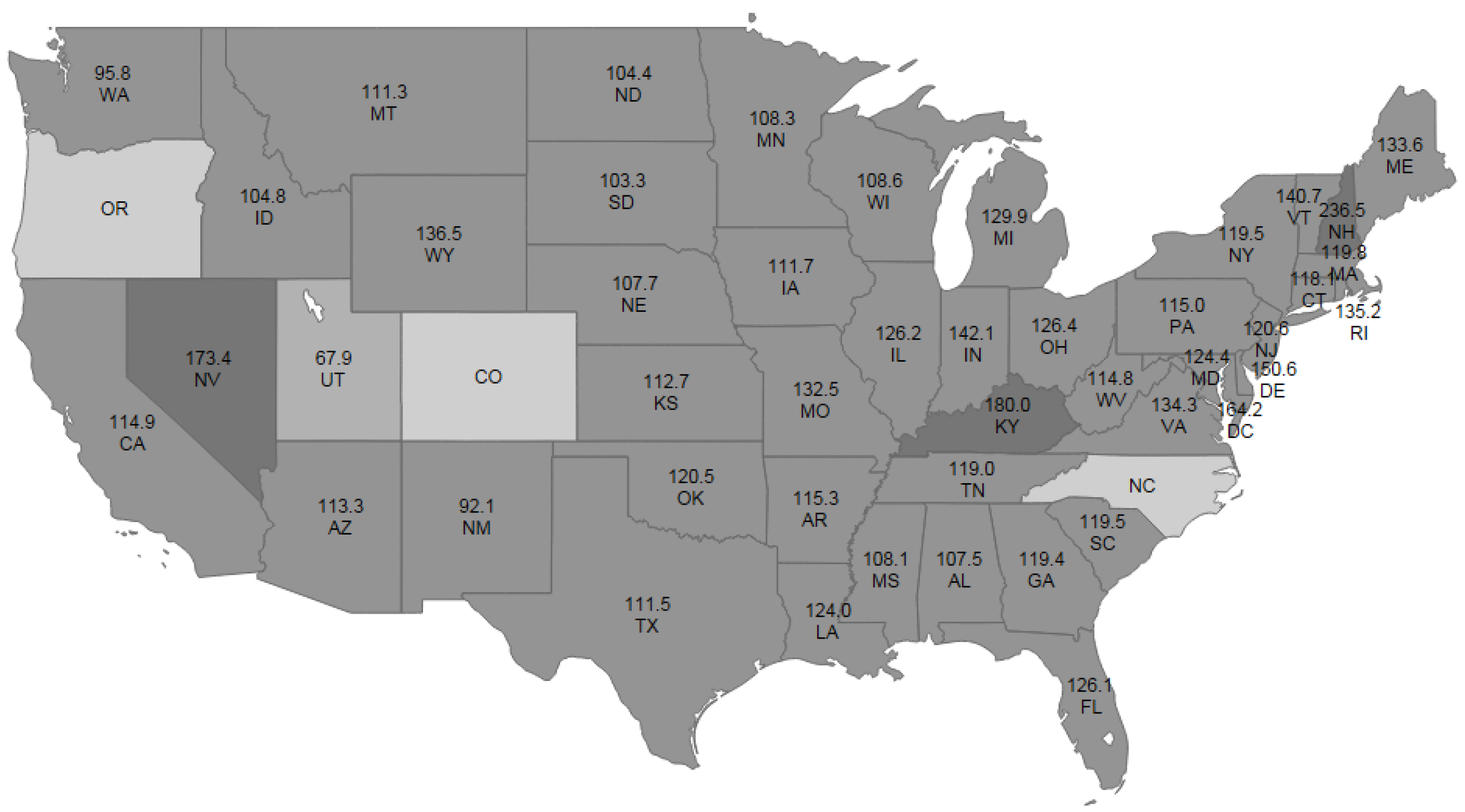The other one is the row-standardized border length weights matrix as suggested in Debarsy et al., (2012) [33].5

Since we are particularly interested in whether the consumptions of cigarettes are spatial correlated and how they are correlated, we plot the average consumption of cigarettes (in packs) per capita over the 30 years for all the states in Figure 1. On the one hand, we see that the cigarette consumptions in some states are negatively correlated with those of its neighboring states. For example, Utah, which has a high percentage of Mormon population,6 has the lowest consumption of cigarettes, with the average consumption to be 67.9 packs per capita per year. In sharp contrast, the consumption of cigarettes in Nevada is nearly 2.6 times of that of Utah, and this could be attributed to the fact that Nevada is a highly tourist state with many casinos. The cigarette consumption in Utah is negatively correlated with those of its neighboring states. This similar pattern also hold for Nevada, New Mexico, Kentucky, and New Hampshire. On the other hand, we see that the consumptions of cigarettes among many other states tend to be similar and thus positively correlated, examples include Iowa, Wisconsin, Pennsylvania, Alabama, Georgia, and so on. The overall spatial dependence is not clear and we will use the formal regression analysis to assess it below.

Figure 1. Average Consumption of Cigarettes (in packs) per Capita per Year by States, 1963–1992.

Figure 1. Average Consumption of Cigarettes (in packs) per Capita per Year by States, 1963–1992.

Before the regression analysis, we first perform the diagnostic procedures and the results are summarized in Table 9. The first row in Table 9 shows that the joint null hypothesis $H_0^a$ is strongly rejected, thus the classical pooled panel data model not appropriate for this data set, and the OLS estimator is biased. The next four rows show that the random effects model is strongly favored against the pooled panel data model, regardless of the assumptions imposed on the spatial parameters. Next, when we test for the spatial error effect and the spatial lag effect jointly, the values of $L{M}_f$ and $L{M}_g$ show that the null hypothesis $\rho =\lambda =0$ is rejected no matter we assume ${\sigma }_{\mu }^2=0$ or allow for the case ${\sigma }_{\mu }^2>0$. This points us to a random effects model with at least one type of spatial effects. In the next six rows, we focus on testing for the spatial error correlation. Although these test statistics unanimously reject the null hypothesis $\rho =0$ in favor of a model with spatial error correlation, we point out that the appropriate statistics should be $L{M}_j$, $L{M}_j^{*}$, and $L{M}_k$ given the presence of random effects but not spatial lag dependence yet at this stage. Finally, we test for the spatial lag dependence, the results in the last six rows suggest rejecting the null hypothesis of no spatial lag dependence, although there is a small value of $L{M}_l^{*}$. Given that the random effects and the spatial error correlation are present by results above, we point out that the appropriate statistics should be $L{M}_l^{*}$, $L{M}_n^{*}$, and $L{M}_o$. From the estimation results in Table 10, the estimated ρ is between $0.353$ and $0.622$ and thus it is not proper to consider such value of ρ as local deviation from 0. As a result, the robust LM tests do not apply. We are left with $L{M}_o$, and it points to the presence of spatial lag dependence. In the following, we first estimate the random effects model with spatial error correlation using two types of spatial weights matrices, then we add in the spatially lagged dependent variable as suggested by our test statistics.

The estimation results are summarized in Table 10. The first column provides the OLS benchmark estimation result for comparison purpose. Although it is biased, all the parameter estimates have expected signs. Price has a negative effect on the consumption of cigarettes per capita, and the disposable income per capita has a positive effect on the consumption of cigarettes per capita, which are consistent with the standard consumption theory. In Columns 2 and 4, we include the spatial error correlation for the two different spatial weights matrices. Compared to the OLS estimates, the price and income elasticity all become smaller in magnitude but have the same signs. The estimated spatial error correlation are positive as $0.353$ and $0.364$, which do not differ much for the two different spatial weights matrices. In Columns 3, 5, 6, and 7, we estimate the full model with different combinations of the weights matrices. The estimates for the spatial lag dependence is negative and statistically significant, which is consistent with our diagnostic testing results. We thus conclude that the full model is the more appropriate specification, and overall we find that the negative correlation dominates in the spatial dependence among cigarette consumptions.

Table 9. LM Testing Statistics.

	$\mathit{W}\mathbf{=}\mathbf{\text{Rook}}$	$\mathit{W}\mathbf{=}\mathbf{\text{Border}}$	$\mathit{W}\mathbf{=}\mathbf{\text{Rook}}$	$\mathit{W}\mathbf{=}\mathbf{\text{Border}}$
	$\mathit{M}\mathbf{=}\mathbf{\text{Rook}}$	$\mathit{M}\mathbf{=}\mathbf{\text{Border}}$	$\mathit{M}\mathbf{=}\mathbf{\text{Border}}$	$\mathit{M}\mathbf{=}\mathbf{\text{Rook}}$
Joint Test $L{M}_a$	12559 ***	12542 ***	12532 ***	12555 ***
Testing for Random Effects
$L{M}_b$	12471 ***	12471 ***	12471 ***	12471 ***
$L{M}_c$	12207 ***	12260 ***	12260 ***	12207 ***
$L{M}_d$	12471 ***	12530 ***	12471 ***	12530 ***
$L{M}_e$	1354.7 ***	1662.7 ***	1573.1 ***	1457.8 ***
Testing for Spatial Effects
Spatial Error and Lag
$L{M}_f$	88.13 ***	70.78 ***	60.82 ***	83.76 ***
$L{M}_g$	172.81 ***	188.36 ***	174.62 ***	143.68 ***
Spatial Error
$L{M}_h$	76.35 ***	60.72 ***	60.72 ***	76.35 ***
$L{M}_h^{*}$	51.78 ***	42.07 ***	24.47 ***	55.05 ***
$L{M}_i$	32.39 ***	23.68 ***	10.33 ***	38.02 ***
$L{M}_j$	138.96 ***	156.08 ***	156.08 ***	138.96 ***
$L{M}_j^{*}$	126.82 ***	126.41 ***	128.63 ***	81.72 ***
$L{M}_k$	94.01 ***	112.90 ***	99.03 ***	58.83 ***
Spatial Lag
$L{M}_l$	36.35 ***	28.71 ***	36.35 ***	28.71 ***
$L{M}_l^{*}$	11.77 ***	10.06 ***	0.10	7.41 ***
$L{M}_m$	1147.00 ***	1385.40 ***	1028.20 ***	580.53 ***
$L{M}_n$	45.99 ***	61.95 ***	45.99 ***	61.95 ***
$L{M}_n^{*}$	33.85 ***	32.28 ***	18.53 ***	4.72 ***
$L{M}_o$	133.96 ***	283.36 ***	108.62 ***	80.05 ***

* $p<0.1$; ** $p<0.05$; *** $p<0.01$.

Table 9. LM Testing Statistics.

	$\mathit{W}\mathbf{=}\mathbf{\text{Rook}}$	$\mathit{W}\mathbf{=}\mathbf{\text{Border}}$	$\mathit{W}\mathbf{=}\mathbf{\text{Rook}}$	$\mathit{W}\mathbf{=}\mathbf{\text{Border}}$
	$\mathit{M}\mathbf{=}\mathbf{\text{Rook}}$	$\mathit{M}\mathbf{=}\mathbf{\text{Border}}$	$\mathit{M}\mathbf{=}\mathbf{\text{Border}}$	$\mathit{M}\mathbf{=}\mathbf{\text{Rook}}$
Joint Test $L{M}_a$	12559 ***	12542 ***	12532 ***	12555 ***
Testing for Random Effects
$L{M}_b$	12471 ***	12471 ***	12471 ***	12471 ***
$L{M}_c$	12207 ***	12260 ***	12260 ***	12207 ***
$L{M}_d$	12471 ***	12530 ***	12471 ***	12530 ***
$L{M}_e$	1354.7 ***	1662.7 ***	1573.1 ***	1457.8 ***
Testing for Spatial Effects
Spatial Error and Lag
$L{M}_f$	88.13 ***	70.78 ***	60.82 ***	83.76 ***
$L{M}_g$	172.81 ***	188.36 ***	174.62 ***	143.68 ***
Spatial Error
$L{M}_h$	76.35 ***	60.72 ***	60.72 ***	76.35 ***
$L{M}_h^{*}$	51.78 ***	42.07 ***	24.47 ***	55.05 ***
$L{M}_i$	32.39 ***	23.68 ***	10.33 ***	38.02 ***
$L{M}_j$	138.96 ***	156.08 ***	156.08 ***	138.96 ***
$L{M}_j^{*}$	126.82 ***	126.41 ***	128.63 ***	81.72 ***
$L{M}_k$	94.01 ***	112.90 ***	99.03 ***	58.83 ***
Spatial Lag
$L{M}_l$	36.35 ***	28.71 ***	36.35 ***	28.71 ***
$L{M}_l^{*}$	11.77 ***	10.06 ***	0.10	7.41 ***
$L{M}_m$	1147.00 ***	1385.40 ***	1028.20 ***	580.53 ***
$L{M}_n$	45.99 ***	61.95 ***	45.99 ***	61.95 ***
$L{M}_n^{*}$	33.85 ***	32.28 ***	18.53 ***	4.72 ***
$L{M}_o$	133.96 ***	283.36 ***	108.62 ***	80.05 ***

* $p<0.1$; ** $p<0.05$; *** $p<0.01$.

Table 10. Estimation of the Cigarette Demand Function.

Model	OLS	MLE	MLE	MLE	MLE	MLE	MLE
		($\mathit{W}\mathbf{=}\mathit{M}\mathbf{=}\mathbf{\text{Rook}}$)		($\mathit{W}\mathbf{=}\mathit{M}\mathbf{=}\mathbf{\text{Border}}$)		($\mathit{W}\mathbf{=}\mathbf{\text{Rook}}$)	($\mathit{W}\mathbf{=}\mathbf{\text{Border}}$)
						($\mathit{M}\mathbf{=}\mathbf{\text{Border}}$)	($\mathit{M}\mathbf{=}\mathbf{\text{Rook}}$)
${\widehat{\beta }}_0$	2.825 ***	2.918 ***	4.267 ***	2.949 ***	3.737 ***	4.634 ***	3.227 ***
	(0.098)	(0.086)	(0.241)	(0.087)	(0.196)	(0.261)	(0.169)
${\widehat{\beta }}_1$	-0.773 ***	-0.739 ***	-0.867 ***	-0.729 ***	-0.821 ***	-0.851 ***	-0.788 ***
	(0.026)	(0.021)	(0.026)	(0.021)	(0.027)	(0.025)	(0.030)
${\widehat{\beta }}_2$	0.586 ***	0.559 ***	0.645 ***	0.551 ***	0.616 ***	0.628 ***	0.595 ***
	(0.022)	(0.018)	(0.022)	(0.018)	(0.022)	(0.022)	(0.024)
$\widehat{\lambda }$			-0.329 ***		-0.204 ***	-0.388 ***	-0.088 **
			(0.044)		(0.039)	(0.044)	(0.038)
$\widehat{\rho }$		0.353 ***	0.586 ***	0.364 ***	0.510 ***	0.622 ***	0.419 ***
		(0.030)	(0.034)	(0.028)	(0.034)	(0.032)	(0.039)
${\widehat{\sigma }}_{\mu }^2$		0.152 ***	0.140 ***	0.154 ***	0.145 ***	0.140 ***	0.149 ***
		(0.015)	(0.014)	(0.016)	(0.015)	(0.014)	(0.015)
${\widehat{\sigma }}_v^2$		0.075 ***	0.069 ***	0.073 ***	0.071 ***	0.067 ***	0.074 ***
		(0.001)	(0.002)	(0.001)	(0.002)	(0.002)	(0.001)
log-likelihood	450.94	1489.2	1514.7	1502.4	1514.6	1537.9	1491.7

* $p<0.1$; ** $p<0.05$; *** $p<0.01$.

Table 10. Estimation of the Cigarette Demand Function.

Model	OLS	MLE	MLE	MLE	MLE	MLE	MLE
		($\mathit{W}\mathbf{=}\mathit{M}\mathbf{=}\mathbf{\text{Rook}}$)		($\mathit{W}\mathbf{=}\mathit{M}\mathbf{=}\mathbf{\text{Border}}$)		($\mathit{W}\mathbf{=}\mathbf{\text{Rook}}$)	($\mathit{W}\mathbf{=}\mathbf{\text{Border}}$)
						($\mathit{M}\mathbf{=}\mathbf{\text{Border}}$)	($\mathit{M}\mathbf{=}\mathbf{\text{Rook}}$)
${\widehat{\beta }}_0$	2.825 ***	2.918 ***	4.267 ***	2.949 ***	3.737 ***	4.634 ***	3.227 ***
	(0.098)	(0.086)	(0.241)	(0.087)	(0.196)	(0.261)	(0.169)
${\widehat{\beta }}_1$	-0.773 ***	-0.739 ***	-0.867 ***	-0.729 ***	-0.821 ***	-0.851 ***	-0.788 ***
	(0.026)	(0.021)	(0.026)	(0.021)	(0.027)	(0.025)	(0.030)
${\widehat{\beta }}_2$	0.586 ***	0.559 ***	0.645 ***	0.551 ***	0.616 ***	0.628 ***	0.595 ***
	(0.022)	(0.018)	(0.022)	(0.018)	(0.022)	(0.022)	(0.024)
$\widehat{\lambda }$			-0.329 ***		-0.204 ***	-0.388 ***	-0.088 **
			(0.044)		(0.039)	(0.044)	(0.038)
$\widehat{\rho }$		0.353 ***	0.586 ***	0.364 ***	0.510 ***	0.622 ***	0.419 ***
		(0.030)	(0.034)	(0.028)	(0.034)	(0.032)	(0.039)
${\widehat{\sigma }}_{\mu }^2$		0.152 ***	0.140 ***	0.154 ***	0.145 ***	0.140 ***	0.149 ***
		(0.015)	(0.014)	(0.016)	(0.015)	(0.014)	(0.015)
${\widehat{\sigma }}_v^2$		0.075 ***	0.069 ***	0.073 ***	0.071 ***	0.067 ***	0.074 ***
		(0.001)	(0.002)	(0.001)	(0.002)	(0.002)	(0.001)
log-likelihood	450.94	1489.2	1514.7	1502.4	1514.6	1537.9	1491.7

* $p<0.1$; ** $p<0.05$; *** $p<0.01$.

6. Conclusions

In this paper, we propose a panel data random effects models with both spatially correlated error components and spatially lagged dependent variables. We consider diagnostic testing within such a framework. We first derive the joint LM test for the individual random effects, the spatial error correlation and the spatial lag dependence. In practice, applied researchers should first consider this joint test. If the joint null hypothesis cannot be rejected, it is reasonable to adopt the classical pooled panel data model. Otherwise, either the individual random effects, or the spatial error correlation, or the spatial lag dependence must be taken into consideration. Next, we derive a wide range of LM tests for the individual random effects and for the two spatial effects separately. In addition, in order to guard against possible local model misspecification, we apply the Bera and Yoon (1993) [19] principle and construct robust LM tests in some cases. These test statistics complement each other and should be used together in performing diagnostic test to search for the most appropriate model. A small Monte Carlo experiment is carried out and the size and power performances of these test statistics are satisfactory. We further use the cigarette demand data set in Baltagi and Levin (1992) [32] to illustrate our testing procedures.

Some future research directions can be considered. First, for the model specification of spatially correlated error components used in this paper, although it allows for both spatial spillovers of permanent and temporary shocks, it does not permit different intensities of these two shocks. It would be of interest to relax this assumption and further generalize our model (see Baltagi et al., 2013 [12]). Second, one can borrow the ideas in Baltagi and Yang (2013a, 2013b) [15,17] to modify our test statistics in order to remedy distributional misspecifications in finite sample, sensitivity to spatial layout, or to be robust against unknown heteroskedasticity.