Context-Aware Local Optimization of Sensor Network Deployment

Abstract

Wireless sensor networks are increasingly used for tracking and monitoring dynamic phenomena in urban and natural areas. Spatial coverage is an important issue in sensor networks in order to fulfill the needs of sensing applications. Optimization methods are widely used to efficiently distribute sensor nodes in the network to achieve a desired level of coverage. Most of the existing algorithms do not consider the characteristics of the real environment in the optimization process. In this paper, we propose the integration of contextual information in optimization algorithms to improve sensor network coverage. First, we investigate the implication of contextual information in sensor networks. Then, a conceptual framework for local context-aware sensor network deployment optimization method is introduced and related algorithms are presented in detail. Finally, several experiments are carried out to evaluate the validity of the proposed method. The results obtained from these experiments show the effectiveness of our approach in different contextual situations.

1. Introduction

Wireless sensor networks are increasingly used for environment and habitat monitoring, moving objects tracking, transportation, structure monitoring, temperature and humidity control, etc. The application of sensors has dramatically improved data collection from the environment and made it easier, cheaper, and more effective.

In order to better understand and capture a dynamic phenomenon by the sensors, effective coverage of the environment is critical. Sensor network deployment optimization approaches are developed to help achieve this goal. There are different approaches for deployment of sensors in the environment. Random scattering and regular grid-like distribution methods are examples of sensor deployment strategies. Manual deployment is one of the simplest ways, but it does not completely satisfy all the requirements of sensor network deployment missions, like providing optimum visibility of objects inside the network. Moreover, regular or random spreading of sensors uniformly in environments may provide a coverage that does not adequately satisfy the user’s needs.

Sensor network deployment consists in determining which sensor, where, and how it should be installed (e.g., sensor type, position, orientation) in the environment, in order to monitor a given region of interest according to the initial consumptions. A way to achieve this is to use optimization algorithms for maximizing a given coverage function of the sensor networks in the environment, for automatically determining the positions and orientations of the sensors. Spatial coverage of sensor networks has different definitions based on different applications [1,2,3,4,5,6,7]. The visual coverage of a point in the environment by a sensor network means that the point is directly visible by at least one sensor and is located within its sensing range. Failing to meet this condition produces some visual holes in the desired network coverage [2]. Many parameters exist, which directly affect the coverage of a sensor network, for example, relations and interactions among sensors in the network, between sensors and environmental elements, and among the environmental elements themselves. Hence, awareness of the surrounding information may help network coverage optimization by means of sensor deployment. In this paper, such knowledge is introduced, and is called Contextual Information (CI).

Most sensor placement methods proposed in the literature do not consider CI information for sensor network deployment and optimization. These methods often consist of deterministic methods based on simplistic models of the sensors and the environment. Some approaches rely on purely geometrical considerations, most prominent approaches being solutions to art galleries’ problems [8,9,10,11]. Others rely on simple modeling of sensing and communication capabilities, usually as a circle centered on the sensor location, with methods for placing sensors a certain space such that all positions will be adequately covered by at least one or even many sensors. In all cases, the simplifying assumptions made in these methods provide theoretically best, but practically suboptimal, solutions, which do not take into account in enough detail the nature of the environment in which the sensors are deployed, as well as the operating characteristics of the sensors in this environment.

In this paper, we propose to better integrate contextual information in optimization algorithms. The originality of this work relies on precise geographical information integration for accessing candidate placements for sensors. Moreover, this geographical information is used both at different levels, for guiding the developmental process of optimized solutions and for assessing the performance of the final solution. This is really important in our opinion, as it allows the optimization process to be finely guided by the properties of the environment in which the sensors will be deployed. Here, we propose a conceptual framework for context-aware sensor network deployment in order to improve sensor network coverage. The proposed framework considers network and environment elements, their dependencies, and characteristics, and applies mentioned CI for the sensor deployment. Hence, in order to improve the coverage, different rules are defined based on CI to perform different actions such as moving existing sensors, or adding new sensors in the network Next, a local context-aware optimization algorithm is developed based on the proposed framework, which locally optimizes the sensor positions by considering the coverage gain improvement following each action.

The rest of the paper is organized as follows. Section 2 briefly reviews optimization algorithms for sensor network deployment. The concept of context in sensor networks is introduced in Section 3, followed by discussions on context-aware sensor network deployment. In Section 4, a conceptual framework for sensor placement based on Voronoi diagram and contextual information is introduced. Section 5 presents the proposed local optimization algorithm in detail, along with experimentation results in Section 6. The paper concludes in Section 7 with result highlights, summary of the proposed approach, and possible future developments.

2. Optimization Algorithms for Sensor Network Deployment

Efficient sensor deployment is an important issue for exploitation of sensor networks, due to its effect on coverage and communications between the sensors in a network. There are a variety of coverage formulations in the literature depending on the type of coverage needed (e.g., area, points, barrier), the sensor deployment mechanism used (e.g., random or deterministic deployment), and the requested properties of sensor networks (e.g., network connectivity, minimum energy consumption) [12]. In this study, the authors consider the coverage as blanket coverage and sensors as visual cameras. Blanket coverage requires placing a minimum number of nodes in an environment, such that every point of interest in the sensing area shall be adequately covered regarding tasks at hand [1,3]. Optimization algorithms define how a good placement is achieved [3,7,13,14,15,16,17,18,19]. These approaches are generally categorized into global and local optimization methods [17]. Both categories are intended to give the best blanket coverage, but the way each method achieves this objective is different. Global approaches consider the whole physical space to find the desired coverage within the network, while local optimization methods try to find the answer based on some local considerations such as network topology and spatial analysis. On the other hand, local approaches divide the search space into local spaces and search the answer locally. In this study, the position of each sensor is determined based on local coverage improvement. The spatial coverage of a sensor network in global and local models depends both on the spatial distribution of the nodes and the spatial information of the environment embedding the sensor network. This information defines CI that will be involved in our sensor network deployment approach. The most critical limitation of the existing methods is that they do not consider CI information for sensor network deployment and optimization. These methods mostly rely on simplistic models of the sensors and the environment which limits their performance in optimal sensor network deployment.

Here, a new local context aware optimization algorithm is proposed to address some limitations of the existing methods. The proposed algorithm is local and relies on an intelligent local context-aware approach for the deployment of a sensor network. In the following sections, the concept of the “context” and its implications for intelligent deployment of sensors will be explained. Next, based on this definition a conceptual framework for local context-aware sensor network deployment and its implementation is presented.

3. Context and Context-Awareness for Sensor Networks Deployment

In order to develop a context aware method for sensor network deployment we need to consider the implications of the context and context awareness in this work. The concept of context is extensively studied in the literature. Dey et al. [20] define context as any information that can be used to characterize the situation of an entity. An entity can be a person, an object or a place. Others defined context as locations, identities of the people or objects around a user, or subjects related to the time (ex. day, week, or season) [21,22,23,24,25,26]. In this definition, the concept of context is related to the state of the environment and may be changed when that state is changed. In the field of computer applications, Dey et al. [20] recommend three aspects to be considered in the environment when the concept of context is defined: the computing environment, the object environment, and the physical environment. Computing environment include the available processors, storage, input and display devices accessible for object, network capacity and connectivity, while object environment concerns the location, behavior, and neighbors of the desired object. Physical environment includes the environment where the computation takes place.

Figure 1. Three components of context in sensor network deployment.

Figure 1. Three components of context in sensor network deployment.

In order to provide a meaningful definition for the concept of “context” for sensor network deployment, the concept of sensor shall take the role of the main object of interest in such a definition. Here, as formalized in Figure 1, the main object of interest is a sensor. Sensor network is considered as the object environment, which includes information on the sensors, for example, sensor position, orientation, and its spatial relations with other sensors in the network. Physical environment is composed of spatial objects in a given area in which the sensor is placed. It also may refer to the spatial relations among the objects, the specific locations in the environment such as desirable areas to be covered or restricted positions that are forbidden to set up the network (Figure 1). Here, context may also include information on sensor network preferences, objectives, and interests.

Therefore, a comprehensive definition of context in sensor networks domain is proposed as follows: “Context is the whole situation, background, or environment of a sensor network. It includes information on sensor itself, the network, and the physical environment and their interactions in a given time.”

That being said, for a context-aware sensor network deployment we need to identify different contextual information (CI). Knowledge on CI for sensors results in awareness of any sensor on its position, orientation, and relation and interaction with other sensors and the physical environment and helps to hence decide on intelligent actions for sensor network optimization, Figure 2 depicts different levels of CI and their interceptions in a sensor network.

Figure 2. Context definition for the intelligent sensor deployment for a given time.

Figure 2. Context definition for the intelligent sensor deployment for a given time.

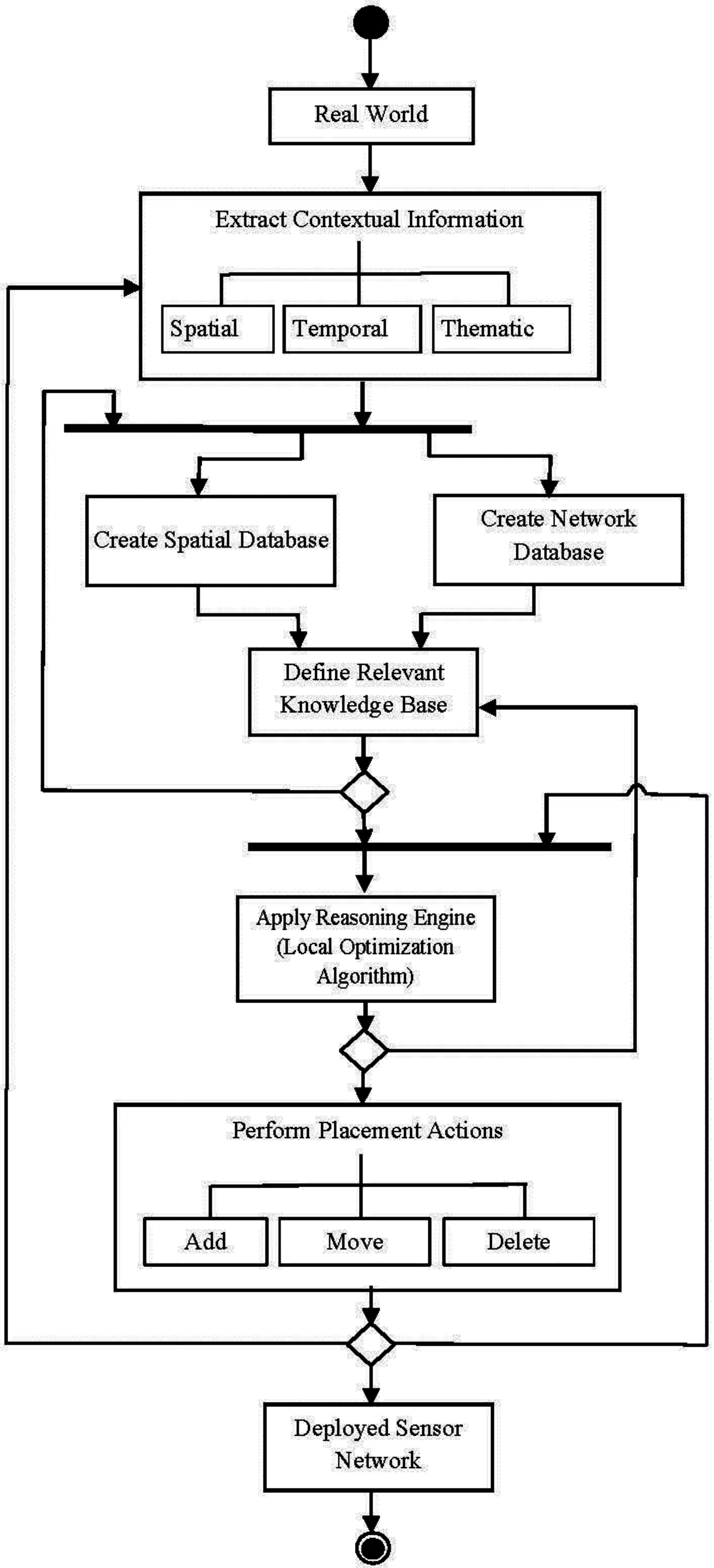
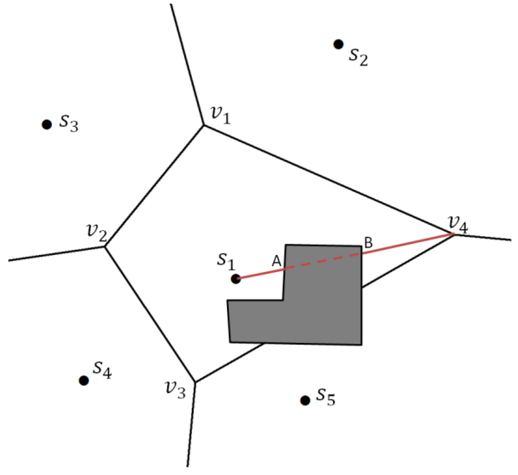
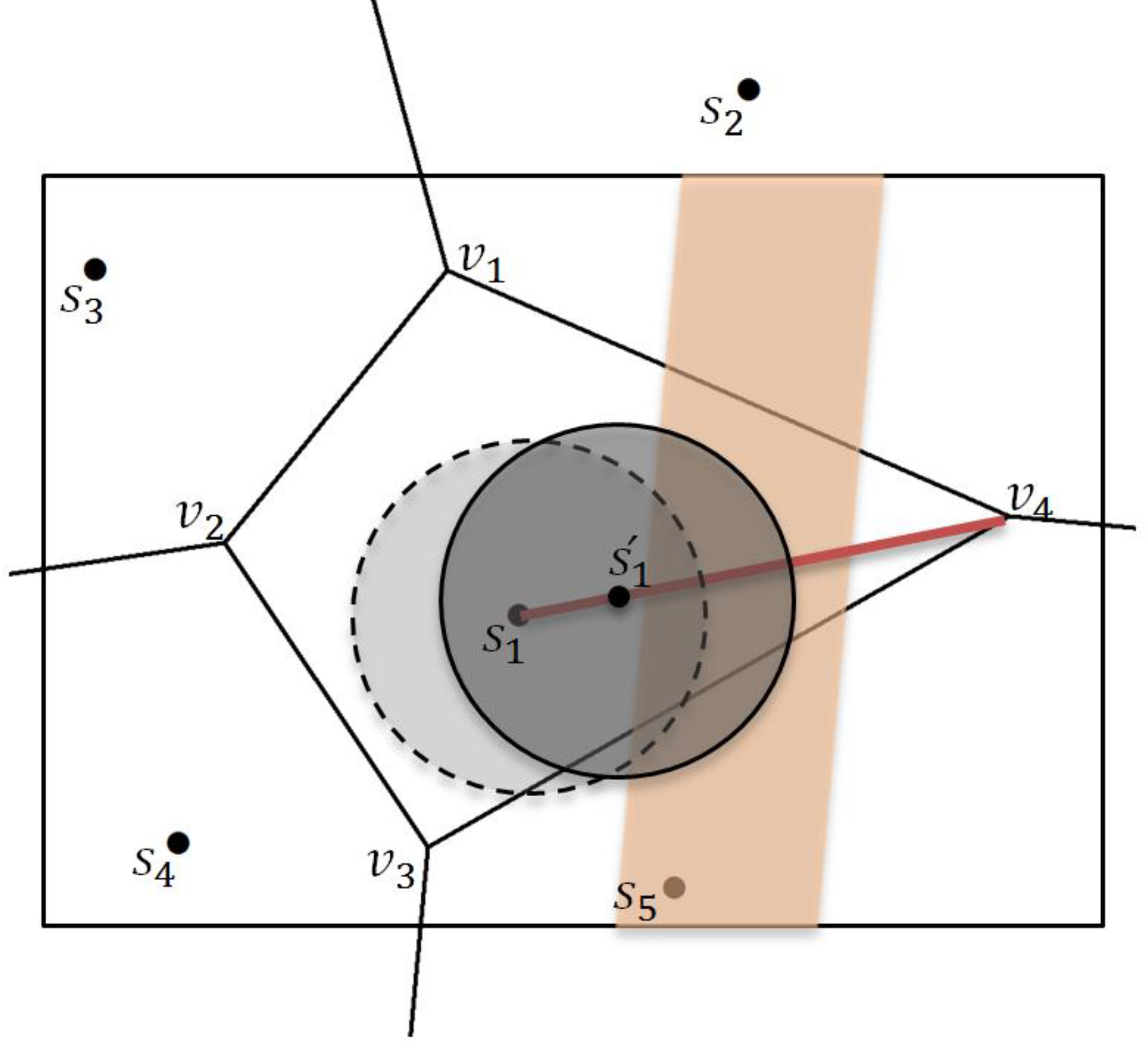
4. A Conceptual Framework for Sensor Network Deployment Using Voronoi Diagram and Contextual Information

In this section, a conceptual framework of sensor network deployment is proposed that applies the introduced contextual information. As explained in Section 2, many optimization algorithms have been used in coverage optimization of sensor network deployment. Some of these algorithms, such as solutions proposed to the Art Gallery problem [27], relies on strong assumptions and considers only a specific element of the environment (e.g., the walls of an indoor environment). Some others, such as derivative-free black-box optimization methods, are not considering explicitly the environmental information, spatial location, and objects around the sensors, although these can be included implicitly in the merit function guiding the optimization. According to Section 3, there are various pieces of information available in each sensor network environment to be considered by the optimization algorithms. The so-called CI will be used in the proposed framework to find good candidate positions of sensor nodes, in order to guide sensor network deployment. Since sensors configuration and their spatial relations may directly impact the optimization process, Voronoi diagram is used in the conceptual framework to model the network environment. It establishes a geometric structure of sensor configuration inside the network as well as the physical environment. It also helps to detect coverage holes in the network, and healing the holes by adding new sensors or moving the existing nodes [16]. A Voronoi diagram for a finite set of points in a given space (here sensors nodes) is a subdivision of the space where every location in the space is assigned to the closet member in the point set. Given a sensor node inside each Voronoi cell, it is supposed that the cell generator (sensor nodes) covers the cell area. Since there are many parameters such as limits on sensor sensing range, and obstacles that bar the line-of-sight between the sensor and sensed objects, gaps and holes inside sensing area will appear. These holes are found by overlapping the Voronoi diagram and the sensor sensing coverage model. Consequently, the CI is included as an essential part of the framework to make it more effective at finding the holes and deciding on the sensor’s adequate actions. The first CI that is considered in this investigation would be the height of spatial elements inside the study area. Argany et al. [16,28] have introduced “enhanced Voronoi-based algorithm”, which used Voronoi diagram as a geometrical structure to optimize the coverage in the network by finding the appropriate positions of the sensors inside the network. The optimum positions in this method were found by moving the sensors toward their new positions by considering specific rules to heal the existing holes. The term “enhanced” in the algorithm refers to the use of information for elevation, line-of-sight, viewshed and etc. as contextual information to improve the sensor’s position. Section 6 presents more details of CI related to different case studies presented later in in this paper.

The contextual information may be very divers in their nature and require different strategies to be categorized in terms of integration in optimization algorithms. CI in sensor network deployment could be classified into spatial, temporal, and thematic information.

-

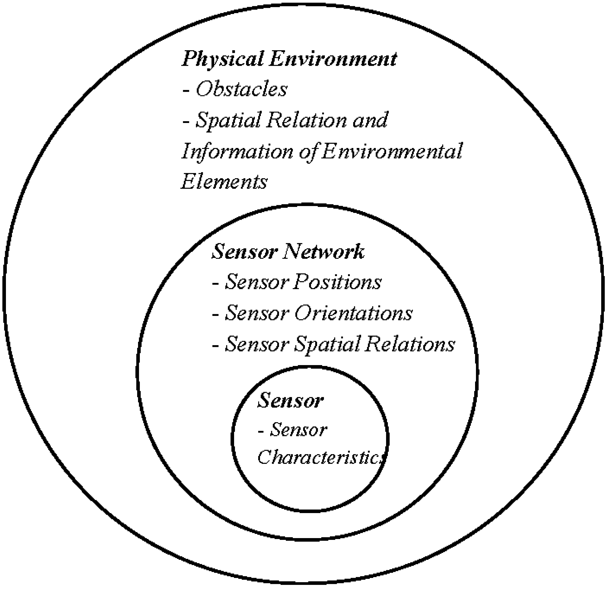
Spatial contextual information refers to the ability of defining objects positions, and geometric relations. Spatial CI is not only about 2D or 3D position of sensors. A comprehensive framework of spatial contextual information may include sensors orientation, movement, routing, targeting, topology, and spatial dependencies and interactions. Hence, all information of spatial relations, interactions, proximity, and adjacency lie in this category.

-

Temporal contextual information concerns the temporal information, and the temporal dependencies in data. Temporal information characterizes the dependency of a situation in the sensor network framework with the time, and also indicates an instant or period during which some other CI is known or relevant. The objects and activities in the physical environment may change. For instance, position or attributes of an obstacle (e.g., its height) may change during a given period of time. A specific example of temporal CI is the information of a sensor movement and its trajectory in the network. Previous actions and movements of a sensor node may provide useful information for the next actions of current sensor or its neighbors.

-

Thematic contextual information in sensor networks constitutes the sensor specifications, network objectives, environment specifics, legal rules, etc. The information regarding the nodes names and roles, and their activity in the network is included in this category. Sensors activities may include measurements of the temperature, humidity, sound, or light. In terms of deployment, the type of sensor movement and its trajectory could be the sensor activity inside the network. Node name should be unique in the network in order to make it possible to be recognized and devolve its roles in multi task networks. Sensor characteristics are sensor specifications, which have been designed during their manufacturing, e.g., their power supply, battery life, sensing range, temperature resistance, dimensions, input and output terminals, processing power, data storage capacity, send and receive information protocols. Network objective expresses the mission of sensor networks to be fulfilled. This objective could be various in multi task networks. It may be varied from covering a whole, or a part of study area to monitor a phenomenon, or sensing different characteristics of the environment. Legal rules define specified terms and conditions for constructing and deploying the sensor networks, e.g., in which locations sensor deployment is allowed, or which parameters are permissible to be measured.

Figure 3. Context-aware sensor network deployment framework.

Figure 3. Context-aware sensor network deployment framework.

Figure 3 presents our proposed context-aware sensor network deployment conceptual framework. The proposed framework has several main components. In the first module, the appropriate CI is extracted from the real world based on tasks at hand. After introducing the CI to the framework, two databases of physical and network environments are created. The spatial database of physical environment includes information of spatial entities such as obstacles, surface elevation and information about restricted areas; while the network database comprises the CI related to sensors and their relations, such as vicinity and topology information provided by Voronoi diagram. The next component is a knowledgebase. The knowledgebase is derived from both databases that provide the necessary knowledge about the sensors, the network and its surrounding environment. This knowledge is provided to the optimization algorithm to better perform the deployment decisions. In the next step, a reasoning engine is applied using the predefined knowledgebase. The reasoning engine may use different move strategies to decide how and in which direction sensors will be displaced (extracted rules). In this work, the reasoning engine is a component of the proposed optimization algorithm, which uses the provided knowledge and information to make a decision on actions to deploy sensors in the environment regarding the initial considerations. In fact, the appropriate actions in the form of extracted rules will be applied. These rules may contain different deployment strategies. For example, suppose that there are some places in the study area with high interest of coverage, but prohibition of sensor installation. Hence, the reasoning engine extract two rules: move sensors toward the regions with high interest of being covered and increase coverage in those areas as much as possible, while preventing sensors to be entered those areas. Therefore, the reasoning engine inside the optimization algorithm may change the deployment process based on provided local contextual information.

These actions may change the topology of the network, the configuration of the adjacent nodes, and consequently, the local coverage. Following each action, local CI of the sensor and its neighbors need to be updated. Hence, some facts and rules may change in the knowledgebase. These local actions carried out iteratively until a desired level of coverage is reached in the network. The process of local optimization in the framework means that network configuration is changed step by step until it obtains its desired configuration considering the spatial, temporal, and thematic contextual information in the network (Figure 3).

5. Implemented Local Context-Aware Optimization Method for Sensor Placement

According to the proposed framework for sensor network deployment, a local optimization algorithm is developed to tackle the sensor placement problem and maximize the spatial coverage of the network. The algorithm utilizes the Voronoi diagram to model the network spatial structure. Here, we propose a generic algorithm to optimize sensor deployment by means of considering local CI to define sensors actions such as movement, deletion, and insertion within the network. The types of CI and their related sensor behavior may be different and are customized according to a sensor network deployment task at hand. Some examples of specific local CI used in some case studies will be introduced and Section 6.

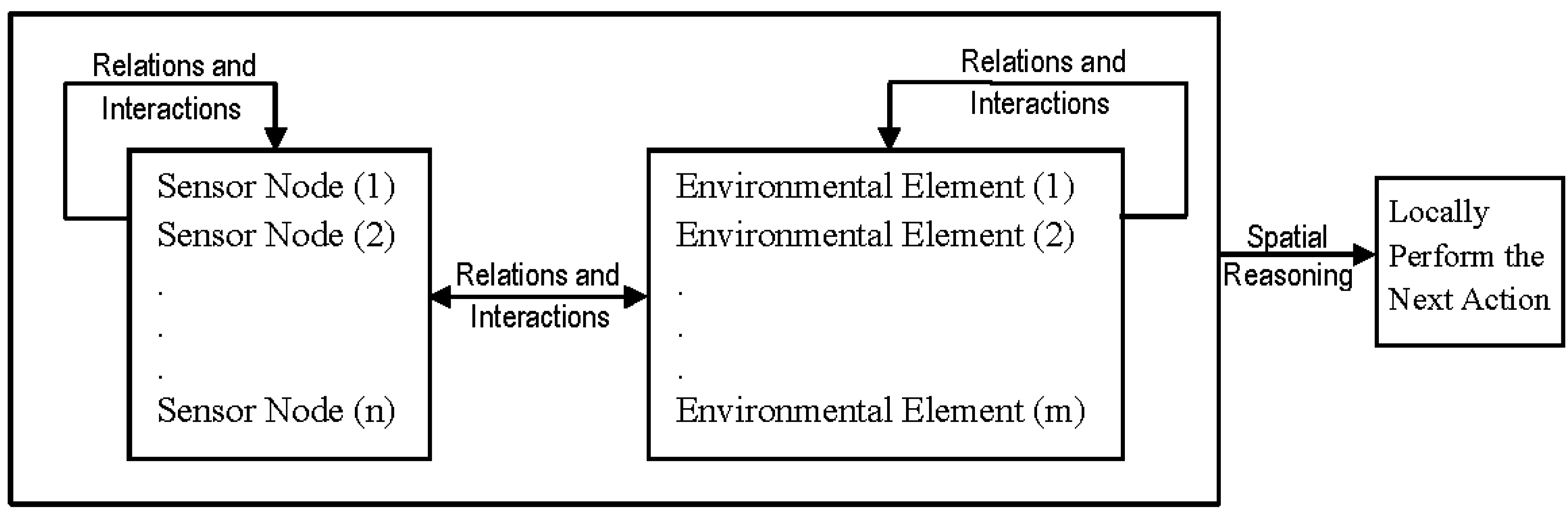
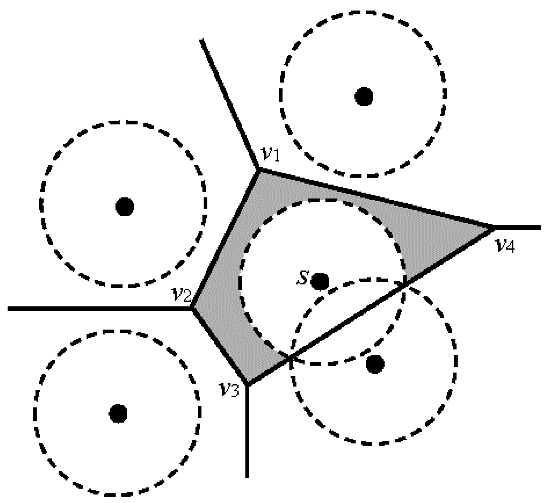
5.1. Formal Presentation of the Local Context-Aware Algorithm

In this section, the proposed algorithm is described in more formal perspective. As illustrated in pseudo-code presented in Figure 4, at the first step of the algorithm, a set of sensors S = {s₁, …, s_n} is deployed randomly in the network. These sensors are then considered as the generators of the Voronoi diagram. Next, the related coverage of each sensor at its initial position is calculated (coverage(s_i)). Meanwhile, different types of coverage may be assumed, which is customized according to the network deployment task at hand. In this study, its simplest form, blanket coverage [29], is used.

Figure 4. The pseudo-code of the proposed local context-aware optimization algorithm.

Figure 4. The pseudo-code of the proposed local context-aware optimization algorithm.

The next step consists of defining the set of context-aware actions (move, add, or delete a sensor) to be considered during the optimization. Section 6 explains how these context-aware actions are defined (Here, for the sake of simplicity, we consider the move action) Next, each possible action is simulated, and local coverage value of each sensor in the network is recalculated:

$$c_i=\mathrm{cov}erage(move(s_i,S)),\forall s_i\in S$$

(1)

Any local move changes the local coverage of a sensor. As a result, the global coverage of sensor network S need also to be updated. The potential gain (g_i) for each move is computed as follows:

$$g_i=\mathrm{cov}erage(move(s_i,S))-\mathrm{cov}erage(s_i,S),\forall s_i\in S$$

(2)

In this step, a greedy algorithm is applied to order the sensors in a priority queue, which means that a simulation of movement has been conducted for all sensors before their permanent move. Sensors are sorted in the priority queue based on their coverage gain following respective simulated moves in the network. Next, the sensor with the best global coverage gain is selected to move locally. Accordingly, for each step, the algorithm is looking for the sensor move with the highest coverage gain based on local CI in the network. Then, ${s^{\prime }}_u$ the new position of the selected sensor (S_u) will be computed regarding the defined context-aware move:

$${s^{\prime }}_u=move(s_u,S)$$

(3)

The next action is to move the selected sensor to its new position. Hence, the network configuration will be changed because of this movement, and as a result, the local adjacency of the sensors may be modified. Accordingly, the set of neighboring sensors of the moved sensor should be determined in the next step. That neighborhood allows updating the coverage values of each adjacent sensor in the priority queue that might be affected by the movement of a sensor. The update operation is then a local operation and hence we do not need to update all the sensors following a local move in the network. Here, two sensors are considered to be adjacent if their respective Voronoi cells are contiguous. It should be noted that if the distance between two neighboring sensor nodes is less than two times the sensing range, then a part of the sensing area will be covered by both sensors between them. Multiple coverage can be introduced and managed as a CI if required. Here, we suppose that each point in the space is covered only by a single sensor.

Next, the sensor with the best coverage gain will be moved. These steps will be run iteratively as long as maximum coverage gain of sensors in the network is greater than a predefined coverage gain threshold (ε).

Figure 5 presents a simplified scenario for a few moves using the proposed local context-aware algorithm execution for deploying five sensors in a flat environment. Red vectors in the figure represent the move direction of the sensor with top priority in each step. In Figure 5a, the sensor in the Voronoi cell A gets the highest rank to move. It may seem that sensor at cell E has the priority to move because of more uncovered space in that cell, but its movement does not have significant impact on coverage gain since the circular sensing area is displaced inside the cell, while the uncovered area will almost remain the same. In Figure 5b, the sensor in the Voronoi cell D is selected to be moved due to the greater area that will be covered compared to other cells, as well as cell B in Figure 5c. In Figure 5d, the sensor inside the cell A has been selected again to move. During this simulation, sensors at cells C and E never get the highest priority to move. This means that the coverage gains of these sensors are always less than the other sensors through this round of optimization. As explained, in cell E there is no overlap between the sensing regions of this sensor and its neighboring sensor cells, then its movement does not have significant impact on the coverage of the network. Sensor at cell C does not get the priority to move, since its cell has been already well covered. A comparison between Figure 5a,d shows that at the end of this round of simulation, the global coverage in the network has been improved.

Figure 5. Simplified simulation of one round of the proposed algorithm to deploy five sensors. Red vector represents the move direction of the sensor with best priority to move in each step. (a),(b),(c), and (d) represent four steps of one round.

Figure 5. Simplified simulation of one round of the proposed algorithm to deploy five sensors. Red vector represents the move direction of the sensor with best priority to move in each step. (a),(b),(c), and (d) represent four steps of one round.

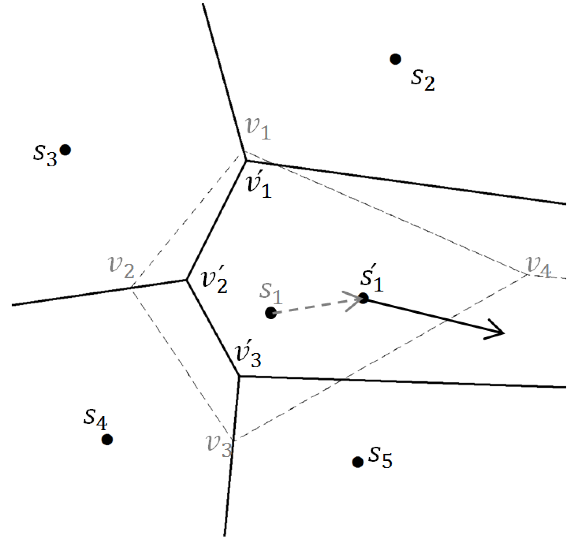
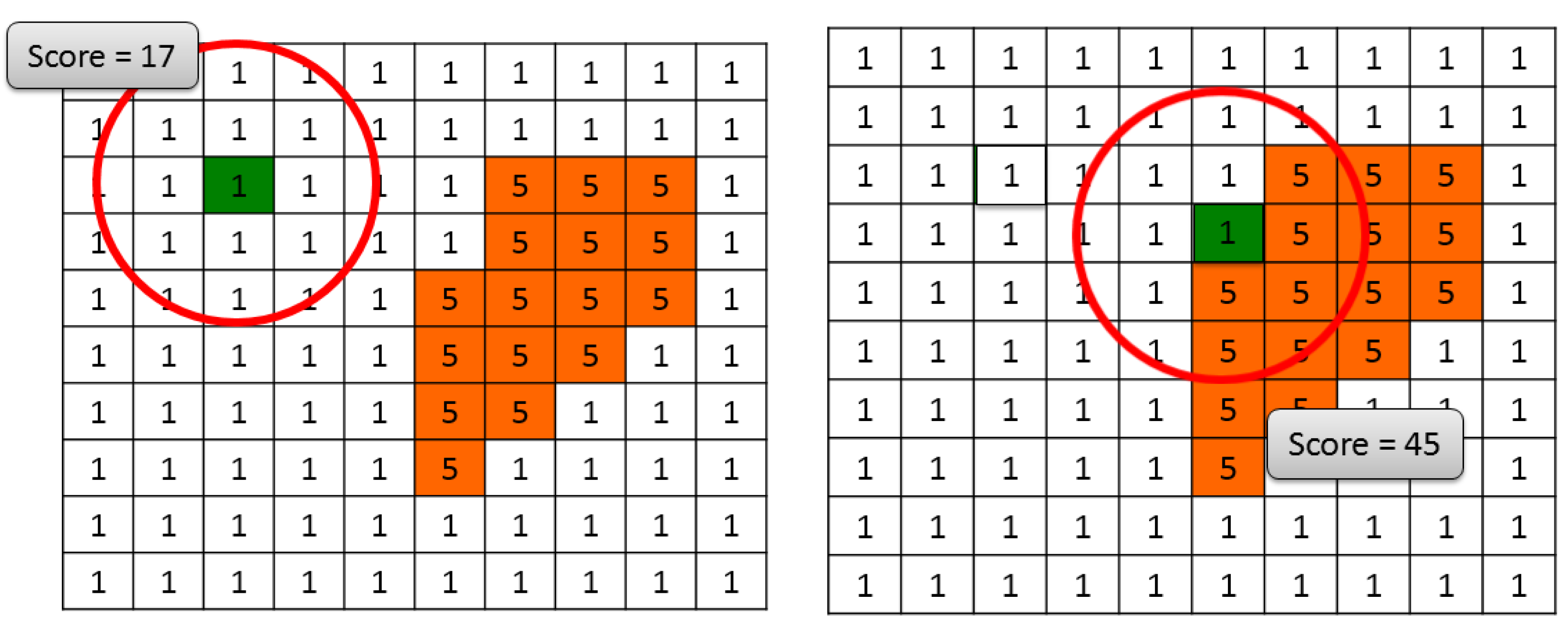
5.2. Strategies for Sensor Movement in the Proposed Local Optimization Algorithm

As stated in the previous sections, different actions are proposed for optimization process depending on local context information for each sensor. These actions may include addition, deletion and movement of a sensor in the network. Moving a sensor is one of the important actions for sensor network optimization. Each move in the proposed deployment optimization approach is composed of two parameters: moving distance and moving direction. Moving distance is determined using a set of rules by the reasoning engine. These rules are defined and stored in the knowledgebase (for more details please refer to Section 6). Orientation of movement is defined based on simple Voronoi diagram.

Before explaining our strategy for determination of moving orientation, we recall the definition of a simple Voronoi diagram. Given a set of two or more finite distinct points in the Euclidean plane, each location is associated in that space with its closest member(s) of the point set with respect to the Euclidean distance. The result is a tessellation of the plane into a set of regions associated with individual members of the point set. This tessellation is called simple “Voronoi diagram” generated by the point set. The regions constituting the Voronoi diagram are referred to as “Voronoi cells”. From the mathematical point of view, consider a finite number of n points in the Euclidean plane with location vector x_i for $i\in \{1,\mathrm{...},n\}$ where all the points are distinct (x_i ≠ x_j for i ≠ j and $i,j\in \{1,\mathrm{...},n\}$). Now, let us consider an arbitrary point p in the Euclidean plane with position vector x, the Voronoi polygon of point p_i is given by:

$$V(p_i)=\left\{x|\Vert x-x_i\Vert \le \Vert x-x_j\Vert forj\ne i,j\in \{1,\mathrm{...},n\}\right\}$$

(4)

For a sensor network, a Voronoi diagram is constructed using initial locations of the sensors. Each sensor in the network is considered as the generator of a cell in the Voronoi diagram, and is responsible for covering the area of its Voronoi cell in the network. In this study, the sensing range for each sensor is considered as a disk with a given radius r around a sensor. Given the circular covered area, and the Voronoi cell of a sensor node, the uncovered area is defined as the symmetric difference of the Voronoi cell and the sensing disk (Figure 6).

Figure 6. Voronoi diagram for five sensors in a network. Dashed circles represent the sensing area of each sensor; the gray region represents the uncovered area of the Voronoi cell associated to the sensor s.

Figure 6. Voronoi diagram for five sensors in a network. Dashed circles represent the sensing area of each sensor; the gray region represents the uncovered area of the Voronoi cell associated to the sensor s.

Suppose that a sensor with a circular sensing area is located at point p_i, and it does not cover V(p_i) completely. Then, some uncovered area within the Voronoi cell exists. In this situation, there are some strategies to heal the holes [16]. Moving the sensor may improve the coverage inside the V(p_i), and hence, the global coverage over the network.

Figure 7. Moving direction and distance changes during the optimization process, dashed line represents the first step of the optimization, and solid line the second.

Figure 7. Moving direction and distance changes during the optimization process, dashed line represents the first step of the optimization, and solid line the second.

The most probable uncovered area inside a Voronoi cell might be in the direction of the farthest Voronoi vertex from the sensor position that generates the cell [16,30]. Hence, the reasoning engine in optimization algorithm uses different move strategies to decide how and in which direction sensors will be moved (extracted rules). The strategy that is used in the proposed algorithm is to move toward the farthest Voronoi vertex on the line $\overline{s_i{v}_{farthest}}$. Thus, for each sensor, an increase of its coverage is expected if the sensor move will be directed toward the farthest vertex in its Voronoi cell. The proposed move may change its direction or distance at each step based on new CI. After each move of a sensor, configuration of the network is changed. Hence, the Voronoi diagram of the network is modified and the adjacency of the moved sensor is updated. That being said, the trajectory of a sensor may not be linear during the optimization process, which means that sensor movements are changed during the iterations, and the improved direction and distance are applied (Figure 7).

5.3. Strategies for CI Integration in the Proposed Local Optimization Algorithm

In the proposed local context-aware optimization algorithm, different actions including addition, move or deletion of a sensor are defined based on local contextual information. Depending on the nature of CI, different strategies may be applied to carry out these actions. In most cases, it is possible to map spatial contextual information and manage them based on a layer based approach. For other types of contextual information, we need to have a different strategy.

For spatial contextual information that can be mapped, two steps are considered for their integration in the optimization process:

First, some CI categories are simulated in different layers as the raster weighted maps. For example, the CI of elevation of environmental elements is represented by a raster map where its pixel values contain the elevation. In another case, the CI of restricted area is represented by a weighted raster map with the values of zero for restricted regions and one for authorized regions. Therefore, the idea here is to represent different CI with different weighted raster maps. In the next section, other examples will be discussed.

In the second step, these raster layers need to be overlaid in the knowledge base to extract appropriate rules. In order to consider different CI layers, a scoring method is used in our proposed algorithm. For example, suppose that there are two types of CI that represent the desirability of coverage for a specific area and another represents the restriction of installing sensor inside that area. Hence, we have two raster maps with two types of weights. The scoring machine overlaid these two weights and gives one score for each pixel. Then, the reasoning engine in the algorithm use these scores to extract the optimization rules and decide how and in which direction sensors will be moved inside the network. These two steps will be more clarified in next section when different case studies are presented.

There are other types of CI presented in Section 4 that cannot be integrated in the proposed algorithm by the weighted raster maps. Information on sensing range and sensing orientation of each sensor in the network is in this category. These CI are managed as introduced facts in the knowledge base that are used in optimization process. The reasoning engine considers these types of CI and integrates them to other local CI during the optimization process.in the algorithm by entering their direct values As an example, distance between neighboring sensors is computed locally at each step. This information is used as CI to avoid coverage overlap between these sensors. The rule that uses this information indicates to the system that if the distance between two sensors is less than the sum of their sensing ranges, then these sensors should be moved away from each other.

6. Different Case Studies for Evaluation of the Proposed Local Context-Aware Sensor Network Deployment Optimization Algorithm

In this section, we present several experiments that demonstrate the capacity of the proposed algorithm to consider different types of CI for sensor network optimization. The study area for our experiments is a part of old Quebec City with a dimension of 180 m by 170 m (Figure 8).

Figure 8. The study area of experiments.

Figure 8. The study area of experiments.

For the experiments, 12 sensors have been assumed to be deployed. The sensors are supposed to be visual cameras with 360° horizontal, ±90° vertical sensing angle, and 35 m of effective sensing range. Placing sensors on the vertices of a triangular lattice is well-known as an optimal solution of deploying sensors over a flat plane [31]. Thus, the initial positions of the sensors were defined on the vertices of a triangular lattice for all different case studies (Figure 9). In one situation, the number of sensors has been increased in order to find the optimal number of sensors needed to cover the entire study region.

For these experiments, we assume that sensors are deployed in an environment with the following considerations that constitute a part of our CI set for the experiments:

-

Spatial positions of environmental elements and obstacles are known,

-

Digital Surface Model (DSM) of the environment is provided,

-

For each sensor, visible and invisible areas are recognized by calculation of line-of-sight and viewshed,

-

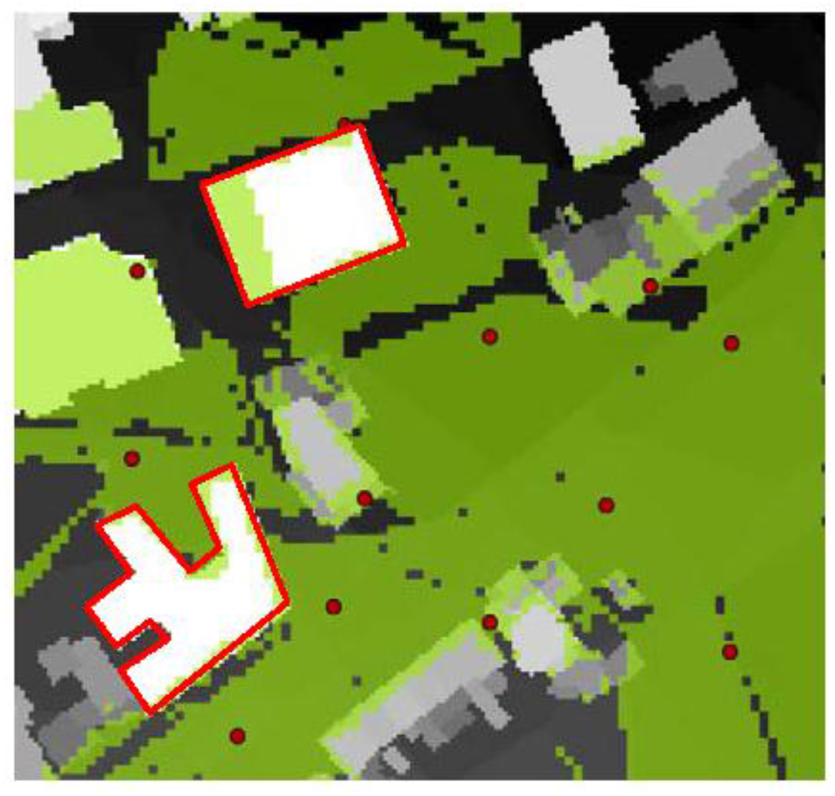
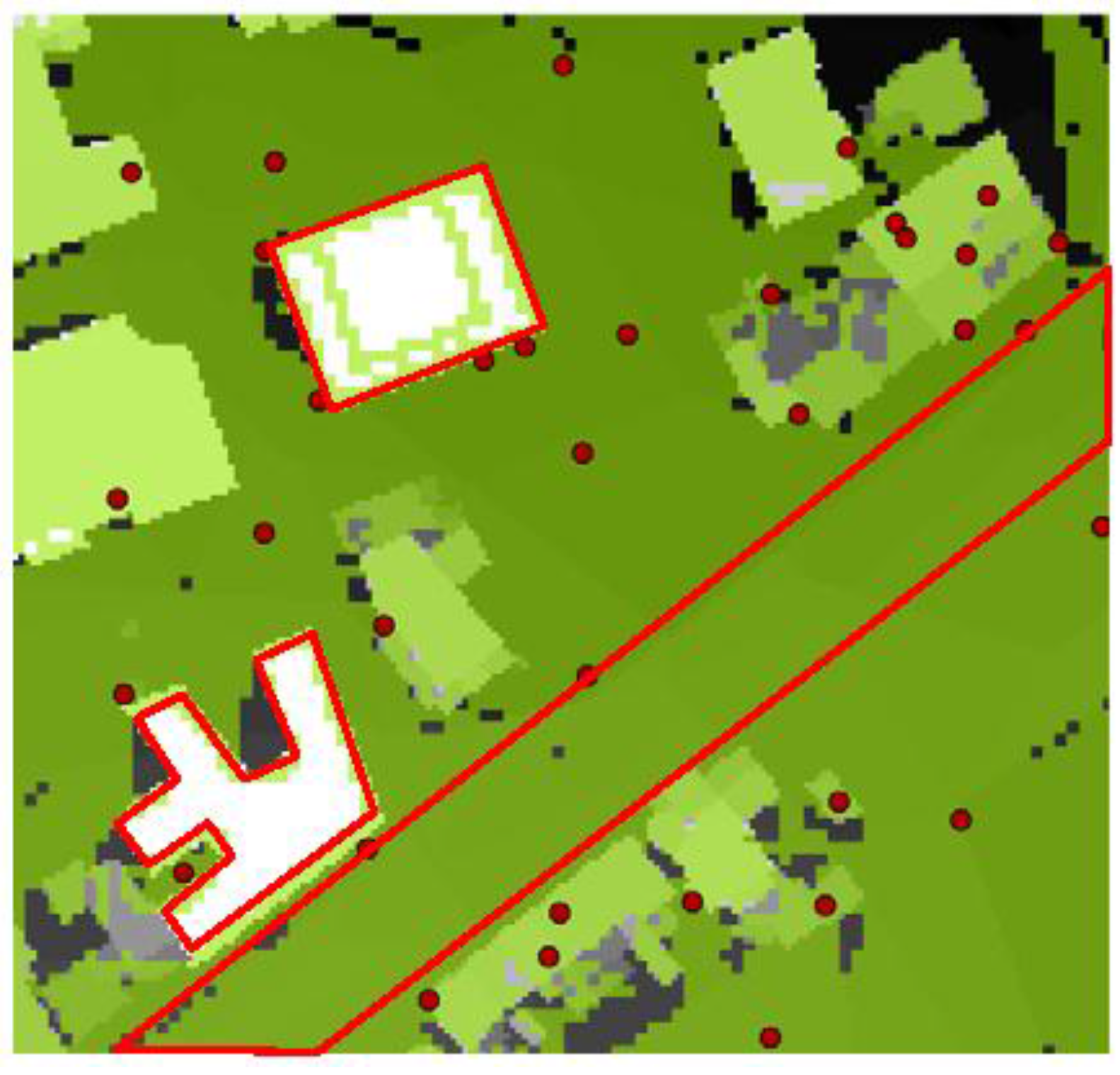
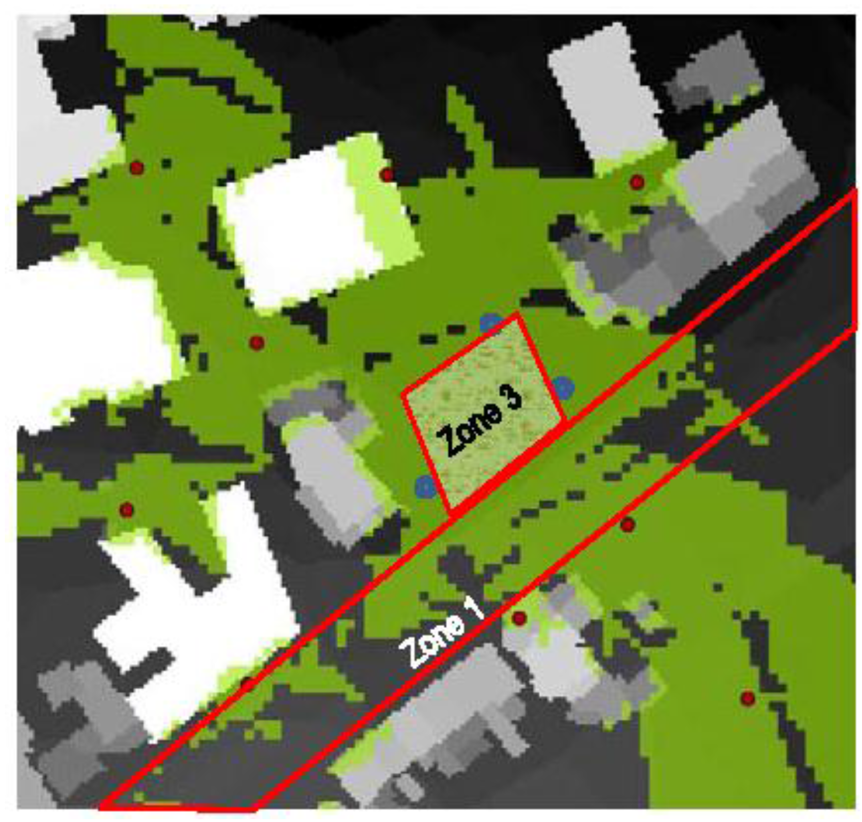
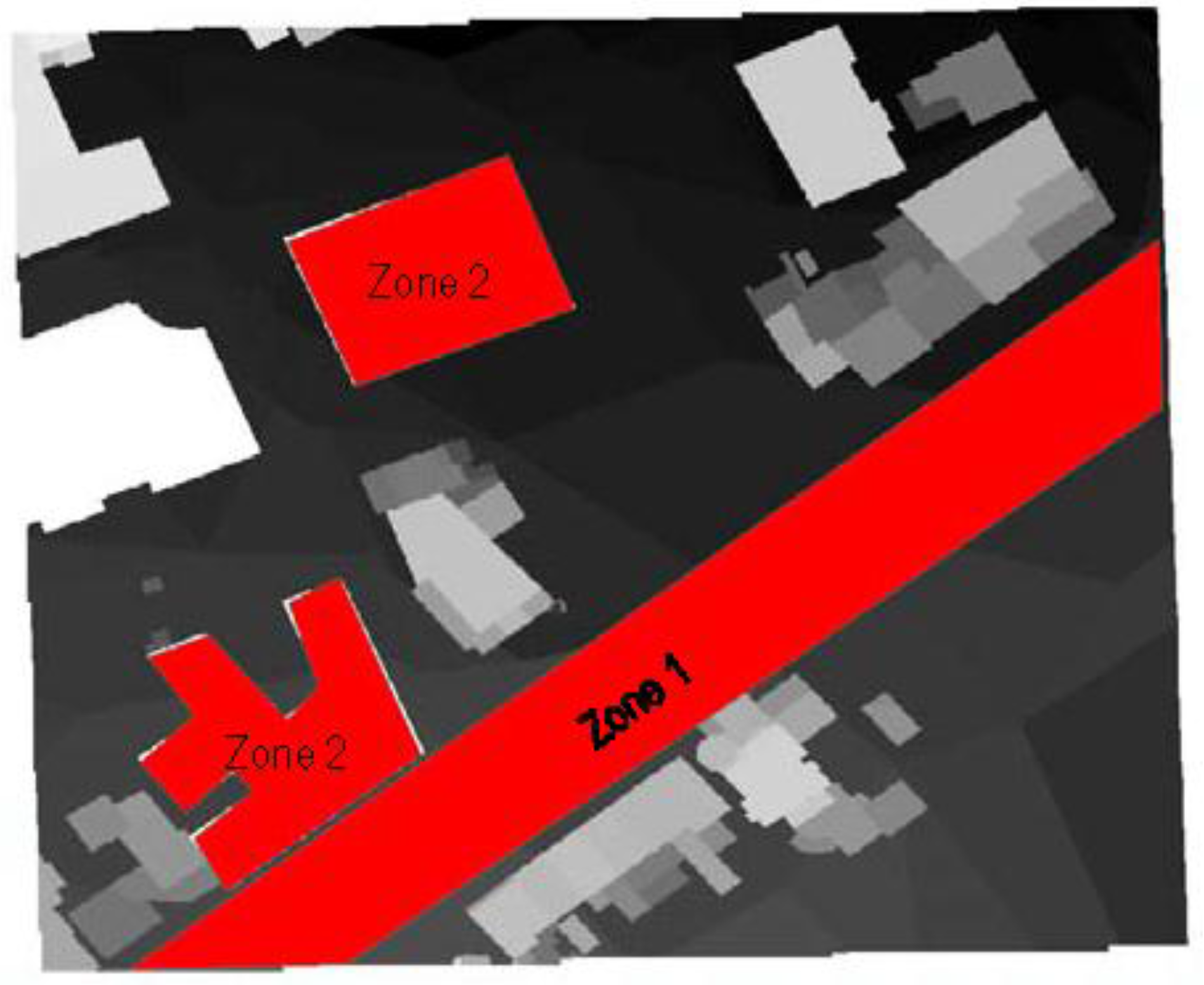
Some restricted zones for sensor installation exist in the study area,

-

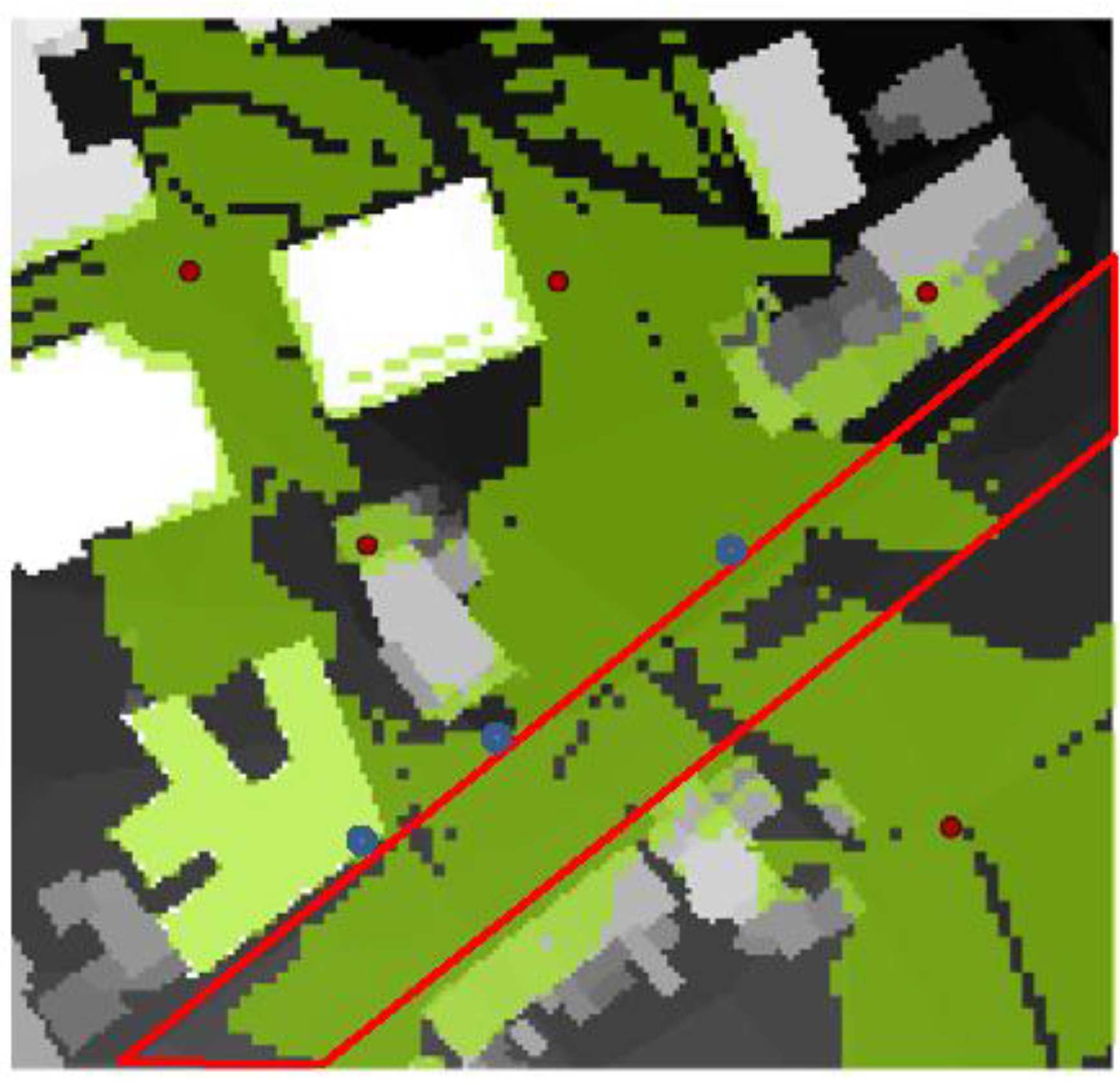
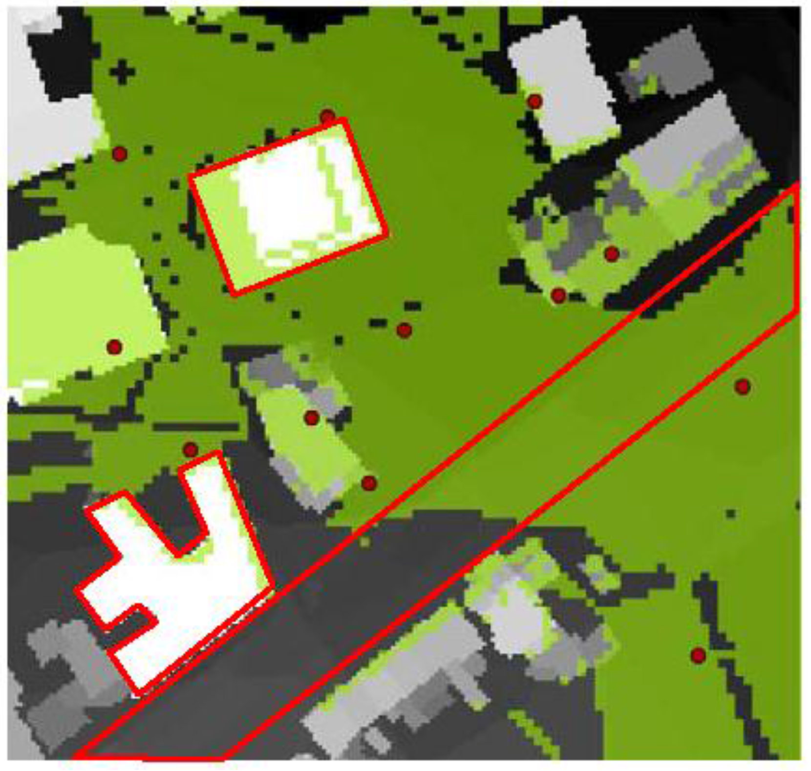
There is a zone with high desirability of coverage, with prohibition for sensor installation,

-

There is a zone with low level of activity, and high desirability of coverage. This zone is located close to a zone with high level of activity but low desirability of coverage. In both zones sensor installation is forbidden.

This CI set will be integrated to the deployment optimization process and will define the way each sensor move locally during the optimization process.

Figure 9. The initial positions of sensors based on a triangular configuration.

Figure 9. The initial positions of sensors based on a triangular configuration.

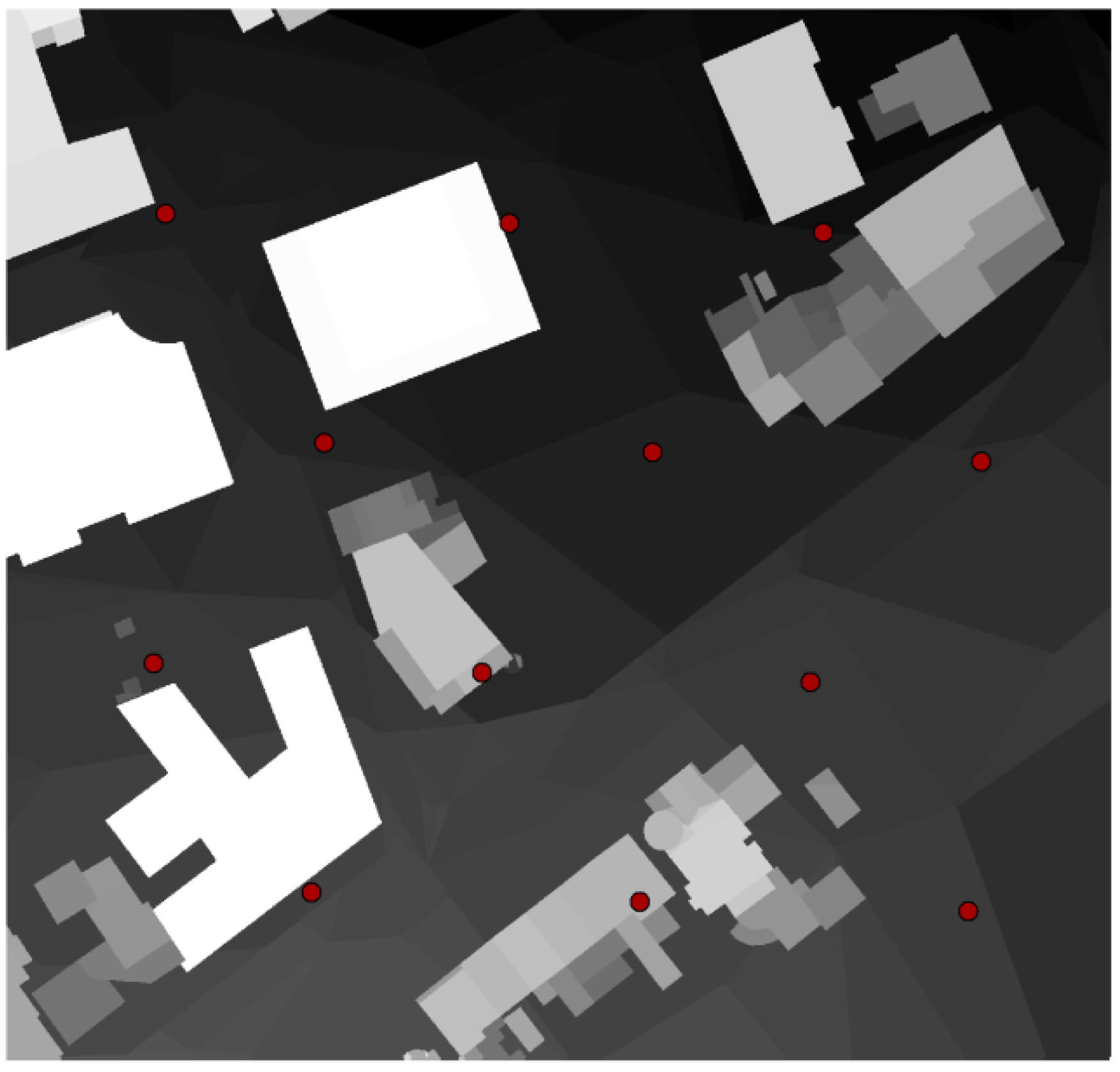
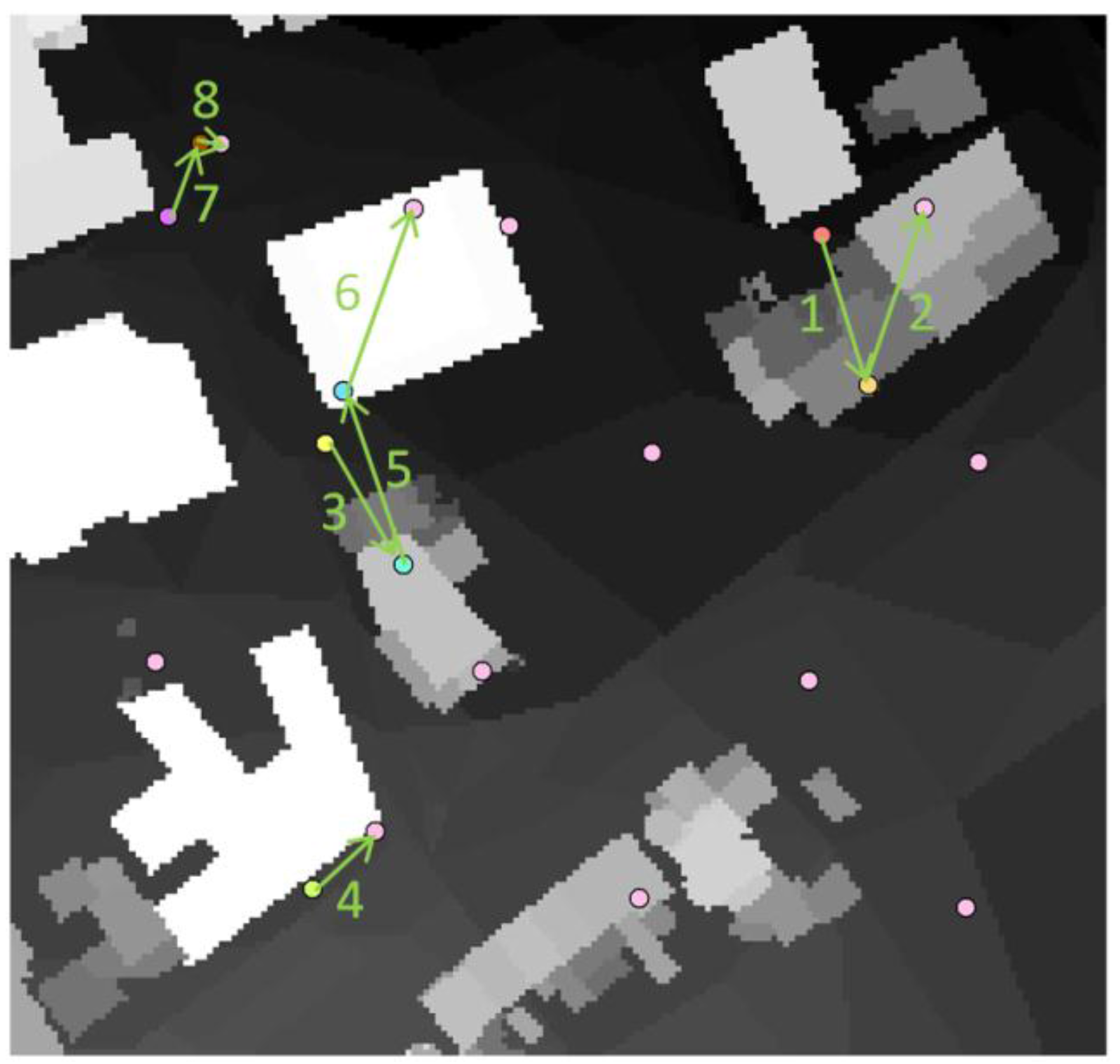
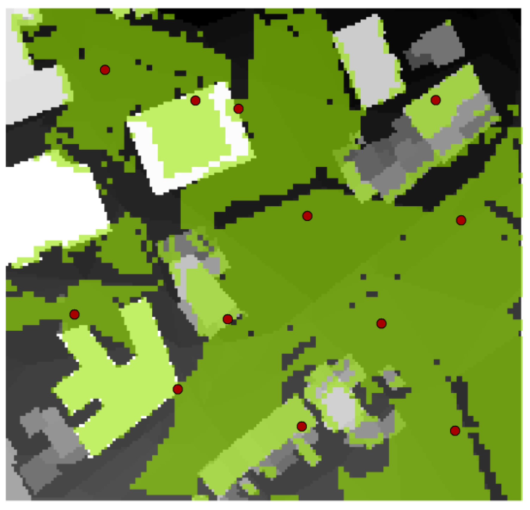
6.1. Optimization Considering the Obstacles and Surface Model as CI

The first category of CI to be considered in deployment optimization knowledgebase is the surface model of the network. Having this knowledge, the elevation details of the study area is provided as well as the obstacles baring the sensing field of the sensors. As mentioned in Section 5.2, the second parameter in a sensor movement is the distance. Here, the sensor is moved toward the farthest Voronoi vertex until it reaches the highest elevation on the line $\overline{s_i{v}_{farthest}}$. Hence, object elevation is considered as spatial CI in the deployment optimization. It is expected that points with the highest elevation provide better coverage compared to points at lower elevation. This CI has been used also in another part of the algorithm, when the viewshed is used to calculate the coverage in the network and consider the obstacles.

As mentioned earlier, we considered 12 sensors to be deployed on the map of old Quebec City using the proposed context-aware optimization algorithm. Figure 10 depicts the movement of sensors for eight iterations. The arrows show the movements’ distance and direction, and the numbers beside each arrow represent the iteration number. Sensors that do not have any arrows beside them have not moved during the optimization process. In this case, four sensors had the potential of improving the network coverage, by considering the mentioned situations to define their displacements. If the rest of the sensors move, they do not improve the coverage adequately regarding the predefined gain threshold. Then, they have remained in their initial triangular lattice positions. This may be explained by the fact that these sensors are located in the area with little height variation, or other sensors movements have had more impact on the coverage improvement or already covered that area. For example, the move number 4 covers all area at the top of the building beside it; this movement of the other sensor at the left side of the building will not have significant impact on the coverage in that area. So, this sensor never stands at the first rank of the priority queue, and as a result it does not move.

Figure 10. Sensor movement simulation of the context-aware optimization algorithm.

Figure 10. Sensor movement simulation of the context-aware optimization algorithm.

Figure 11 depicts the coverage improvement during the optimization process related to the iterations shown in Figure 10. The upward slope of the diagram shows the improvement of coverage over the iterations. The initial overall coverage of the triangular lattice deployment is 58.79% considering the obstacles, and the final coverage obtained from the optimization is 63.46%. It may seem the coverage improvement was negligible. The reason for little difference between the initial and final coverage is due to the triangular lattice initial configuration, which is close to optimum [31]. We may call the obtained coverage not only the improved coverage but also more realistic coverage due to consideration of local CI. Figure 12 shows the final sensor positions and covered regions.

Figure 11. Coverage improvement over iterations of the context-aware method.

Figure 11. Coverage improvement over iterations of the context-aware method.

According to Figure 11, 63.46% of coverage over the study area is reached at the end of the optimization process compared to 59% at the starting point. Here, one may raise this question: is it really a significant coverage improvement compared to the initial coverage before performing the optimization? To answer this question and also evaluate the efficiency of the local context-aware algorithm, a comparison between the results obtained from this method and a well-known global approach called CMA-ES [18] has been conducted. Since there are many CI available that might be considered in the context-aware method, the same conditions were applied to run both algorithms. In current implementation, just obstacles and surface elevation model are considered as the CI. The comparison was made using eight sensors with random initial positions. In order to avoid the impact of initial positions over the final results [17], 32 runs for each method with 32 different initial random positions was performed. Table 1 presents the results of this comparison. The average values of coverage for both methods are two close values, which support the validity of obtained results from the proposed algorithm compared to a well-known optimization approach.

Figure 12. Coverage map of deploying 12 sensors using the context-aware method.

Figure 12. Coverage map of deploying 12 sensors using the context-aware method.

Table 1. Results of Context-Aware and CMA-ES optimization algorithms.

Method	Avg. Coverage (%)	Best Coverage (%)
Context-Aware	51.17	52.83
CMA-ES	49.09	51.33

Table 1. Results of Context-Aware and CMA-ES optimization algorithms.

Method	Avg. Coverage (%)	Best Coverage (%)
Context-Aware	51.17	52.83
CMA-ES	49.09	51.33

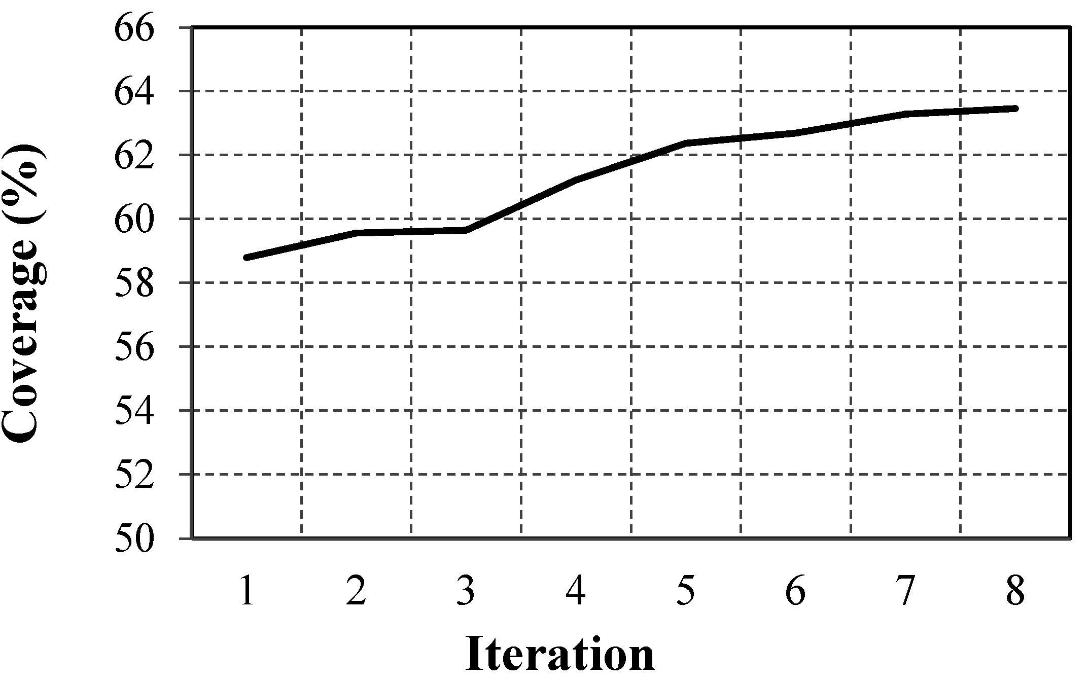
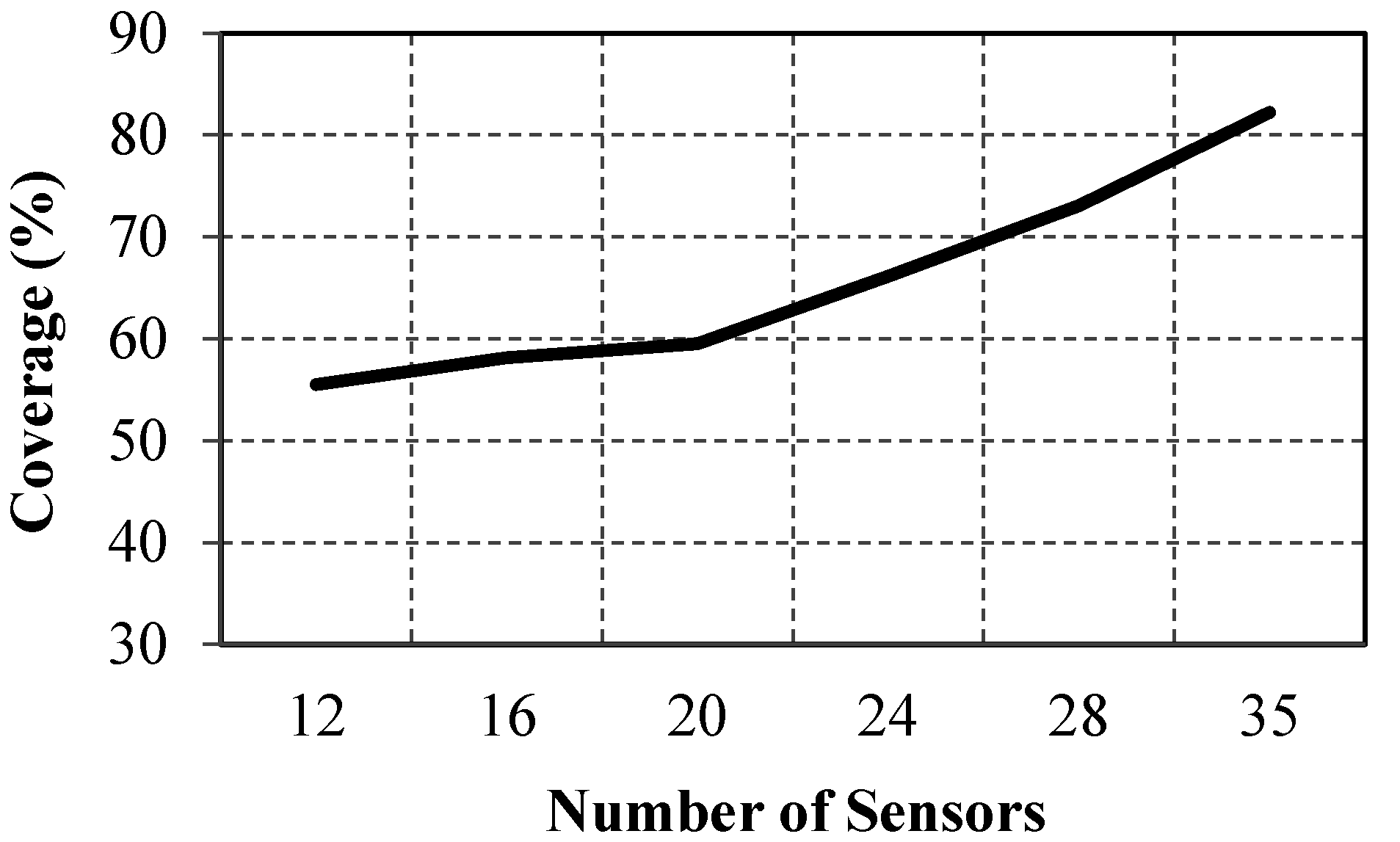
6.2. Optimization Considering the Restricted Area as CI

Thematic information is the next category of CI used in deployment optimization. Many parameters exist in the real environment to be considered in the knowledge base as thematic CI. For example, several locations may be legally forbidden for the deployment of sensors, like private buildings, hospitals, military zones, highways, etc. There are other locations, which are difficult to access, or inaccessible for sensors to be installed, like aqueous zones, lakes, rivers, green spaces, and rough terrains. Considering restricted areas in the knowledgebase, sensor action is changed, and the reasoning engine in the optimization algorithm extracts new rules in form of defining new moves. In this case, sensors still move toward the farthest Voronoi vertex, but stop at position ${s^{\prime }}_i$ on $\overline{L_i}$, which $\overline{L_i}$ are the positions on $\overline{s_i{v}_{farthest}}$ excluding restricted areas R from possible sensor positions. So, compared to the previous case study, the direction and orientation of a move here are the same, but the stopping position might be different. Considering elevation as previous CI, the optimization algorithm returns the stopping position as the highest elevation on $\overline{L_i}$ using both pixel values from the map of elevation (DSM) and map of restricted areas.

$$\overline{L_i}=\{p\in \overline{s_i{v}_{farthest}}|p\notin R\}$$

(5)

$${s^{\prime }}_i=\underset{p\in \overline{L_i}}{\arg \max [elev(p)]}$$

(6)

where elev is a function that returns the elevation of position p on the line $\overline{L_i}$.

Suppose that there is a building that has barred the connecting line between s₁ and v₄ on the line $\overline{AB}$ (Figure 13). Then the stop position of the move will be a position on $\overline{s_{1}A}$ or $\overline{B{v}_4}$, depending on weight values represent other types of CI such as elevation, or parameters explained afterward in next subsections.

Figure 13. Sensor’s move representation in case of considering the restricted area. Searching locations have been limited to lines s₁A and Bv₄.

Figure 13. Sensor’s move representation in case of considering the restricted area. Searching locations have been limited to lines s₁A and Bv₄.

To evaluate integrating restricted area, two buildings and a street have been assumed as prohibited locations for installing the sensors (red zones in Figure 14).

Figure 14. Illegal zones of sensor deployment: the street (Zone 1) and the buildings (Zone 2).

Figure 14. Illegal zones of sensor deployment: the street (Zone 1) and the buildings (Zone 2).

Firstly, the street (Zone 1) was considered as a CI constraint forbidden from having sensor in it, and the optimization algorithm was run to deploy 12 sensors, which had been initially deployed on a triangular lattice grid, and overall coverage value of 56.19% was obtained. Final positions of the sensors and the covered region have been represented at Figure 15. As expected, there are no sensors located on the restricted street.

Figure 15. Coverage map of 12 sensors using the local context-aware method, considering the street (Zone 1) as the restricted area without sensors (the red border zone).

Figure 15. Coverage map of 12 sensors using the local context-aware method, considering the street (Zone 1) as the restricted area without sensors (the red border zone).

Figure 16. Coverage map of deploying 12 sensors using the context-aware method, considering the buildings (Zone 2) as the restricted area (the red border zones).

Figure 16. Coverage map of deploying 12 sensors using the context-aware method, considering the buildings (Zone 2) as the restricted area (the red border zones).

In the second phase of this implementation step, two buildings (Zone 2) have been added as the restricted areas and the street in the former step was considered as an authorized region. Similar to previous tests, the optimization algorithm was run over 12 sensors with the triangular lattice initial positions, and 59.48% of coverage was obtained. The results are represented in Figure 16. There are no sensors on the restricted buildings, despite the higher elevation on those regions. Compared to the previous case better coverage results are returned, when the street has been introduced as a legal place to install the sensors. Hence, the street might be taken into account more critical compared to the buildings in terms of installing the sensors for improving the coverage. This conclusion would be clear, because the area of buildings is less than the area of street in this study region. In fact, in this case, putting sensors at the top of those buildings covers just the roofs since the sensing range is a short 35 m range.

Finally, two buildings and the street (Zones 1 and 2) were entered to the algorithm as the CI of unauthorized areas. Initial parameters to run the algorithm are the same as earlier experiments. The coverage value is 55.52%. The outcome is presented in Figure 17. Adding CI as the weighted maps, expresses the ability of context-aware algorithm to accept different CI separately or together in different case studies according to the application requirements.

Figure 17. Coverage map of deploying 12 sensors using the context-aware method, considering the street (Zone 1), and buildings (Zone 2) as the restricted area (the red border zones).

Figure 17. Coverage map of deploying 12 sensors using the context-aware method, considering the street (Zone 1), and buildings (Zone 2) as the restricted area (the red border zones).

In the following, we study to find the impact of increasing the number of sensors over the coverage value of the network, considering both Zones 1 and 2 as the restricted areas. It started with 12 sensors and increased the number of sensors up to 35. The initial positions in all cases have been placed on the triangular lattice configuration. Table 2 shows the results of the implementations. In order to calculate the maximum possible coverage over the study area, the maximum coverage should be specified. Considering the area of the restricted buildings, the remaining region is 92.53% of the entire study area. Since sensors may move close to the street during the optimization process and make it covered, its area was not in calculation of the percentage of the maximum feasible covered region. Compared to the street, buildings do not have this characteristic due to their height. Hence, moving sensors close to buildings does not make them covered. Based on results presented in Table 2, almost all regions of the study area have been covered using 35 sensors. Figure 18 depicts the improvement of coverage by increasing the number of sensors over the study area. Figure 19 shows the configuration of the deployed sensors in the network and the covered area. Many buildings exist at top-right and bottom region of study area, which cause presenting high density of sensors. This may be also interpreted according to the restricted areas, in which sensors cannot be deployed, and push forward to cover the regions that are more complex.

Table 2. Impact of increasing the number of sensors on the coverage using context-aware method in case of considering the restricted area (Zones 1 and 2).

Num. of Sensors	12	16	20	24	28	35
Coverage (%)	55.52	58.15	59.51	66.14	73.08	87.56
Num. of Iteration	11	8	9	19	15	34

Table 2. Impact of increasing the number of sensors on the coverage using context-aware method in case of considering the restricted area (Zones 1 and 2).

Num. of Sensors	12	16	20	24	28	35
Coverage (%)	55.52	58.15	59.51	66.14	73.08	87.56
Num. of Iteration	11	8	9	19	15	34

Figure 18. Impact of number of sensors on the coverage obtained by the context-aware method in case of considering the restricted area (Zones 1 and 2).

Figure 18. Impact of number of sensors on the coverage obtained by the context-aware method in case of considering the restricted area (Zones 1 and 2).

Figure 19. Coverage map of deploying 35 sensors using the context-aware method, considering the street (Zone 1), and buildings (Zone 2) as the restricted area (the red border zones).

Figure 19. Coverage map of deploying 35 sensors using the context-aware method, considering the street (Zone 1), and buildings (Zone 2) as the restricted area (the red border zones).

6.3. Optimization Considering Desirability of Coverage in a Given Area as CI

Desirability of coverage is another type of thematic information that can be considered in the knowledgebase for the optimization process. Suppose that there are some places in the study area, where sensors cannot be set up, but there is a high interest in covering those regions. Then, the weighted map for this CI is defined as follows. Given an environment $\mathrm{\Xi }$, let C_i be the circular sensing region with the radius r of sensor s_i centered at the position p_i:

$$C_i=\{p\in \mathrm{\Xi }|\Vert p-p_i\Vert \le r\}$$

(7)

Suppose that positions are corresponding to pixels, then to define the places with higher concern of coverage the w_dc is defined as the weight of desirability of the coverage in the environment $\mathrm{\Xi }$. Evidently, the places with higher desirability of coverage should get higher weight (w_dc) compared to the rest of the study area, e.g., the street in Figure 20. To consider this weight in the sensor move, each possible new sensor position p_i gets a score, which is the sum of weights within C_i.

$$scor{e}_{dc}(p_i)={\displaystyle \sum _{p_j\in C_i}{w}_{dc}}(p_i)$$

(8)

Figure 20. Sensor’s move representation in case of considering circular coverage and desirability coverage at the pink area (street), s₁ represents the initial sensor position, ${s^{\prime }}_1$ represents the position with highest weight score on the line s₁v₄.

Figure 20. Sensor’s move representation in case of considering circular coverage and desirability coverage at the pink area (street), s₁ represents the initial sensor position, ${s^{\prime }}_1$ represents the position with highest weight score on the line s₁v₄.

The new rule extracted by the reasoning engine is to move sensors toward the desired region to cover it as much as possible, while sensors should not enter the zone. As in previous experiments, each sensor moves on $\overline{s_i{v}_{farthest}}$, but to respect the new rule, it stops at the position ${s^{\prime }}_i$ with the maximum $scor{e}_{dc}$. In this case, the constraint presented in Section 6.2 needs to be already checked, and as a result the stop position should be out of the restricted area as well.

$${s^{\prime }}_i=\underset{p_i\in \overline{L_i}}{\arg \max (scor{e}_{dc}(p_i))}$$

(9)

Figure 21 shows how a simulated weight map has been created to consider the CI of desirability of coverage. It represents how the score_dc is calculated followed by the movement of a sensor in green cell toward a position with higher score (orange zone).

To evaluate the performance of the method when the desirability of coverage has been considered in a specific area, the optimization algorithm was run over 12 sensors with a triangular lattice initial position. Zone 1 was introduced as the area with high interest to be covered, while it is unauthorized for sensors to be installed. Figure 22 represents the final sensor positions and the covered area. Compared to the case of deploying 12 sensors without introducing any restricted area (Figure 12), and deploying 12 sensors considering Zone 1 as the unauthorized region, results show how six sensors among all, which were closer to Zone 1, have moved and stopped beside the street to make it covered (Blue dots on Figure 22). Overall coverage of 58.48% has been obtained. In this case, the street area has been almost covered. Having covered the desired region with 12 sensors, the question may arise whether the desired region could be covered using fewer sensors deployed in the study area. It means the desired region will be covered applying less optimization process. To evaluate this assumption, the algorithm was run over eight sensors with the triangular lattice initial position. Figure 23 presents the final sensor positions and the covered area. Overall coverage of 49.57% has been obtained. The orientation of the sensors in Figure 23 shows that they were deployed with the purpose of covering the street (red border) as well as maximizing the overall coverage. The blue dots sensors have been moved to cover the desired area, while other sensors have been configured to cover the rest of study area. For example, a sensor at the right side of the street has come closer to the street during the optimization, but not too close like other sensors at the left side, because it belongs to an area with fewer obstacles on the terrain. Thus, if it comes closer to the street to cover an area, which has been already covered by another sensor, the coverage may be lost on a previously covered area. Consequently, as explained before, the reasoning engine extracted movement rules to respect both purpose of covering the desired area as well as overall coverage over the network.

Figure 21. Simulation of the score_dc on the weight map, followed by finding a new sensor position regarding the CI of desirability of coverage.

Figure 21. Simulation of the score_dc on the weight map, followed by finding a new sensor position regarding the CI of desirability of coverage.

Figure 22. Coverage map of deploying 12 sensors using the context-aware method, considering the street (Zone 1) as the desired region to be covered (the red border).

Figure 22. Coverage map of deploying 12 sensors using the context-aware method, considering the street (Zone 1) as the desired region to be covered (the red border).

Figure 23. Coverage map of deploying eight sensors using the context-aware method, considering the street (Zone 1) as the desired region to be covered (the red border).

Figure 23. Coverage map of deploying eight sensors using the context-aware method, considering the street (Zone 1) as the desired region to be covered (the red border).

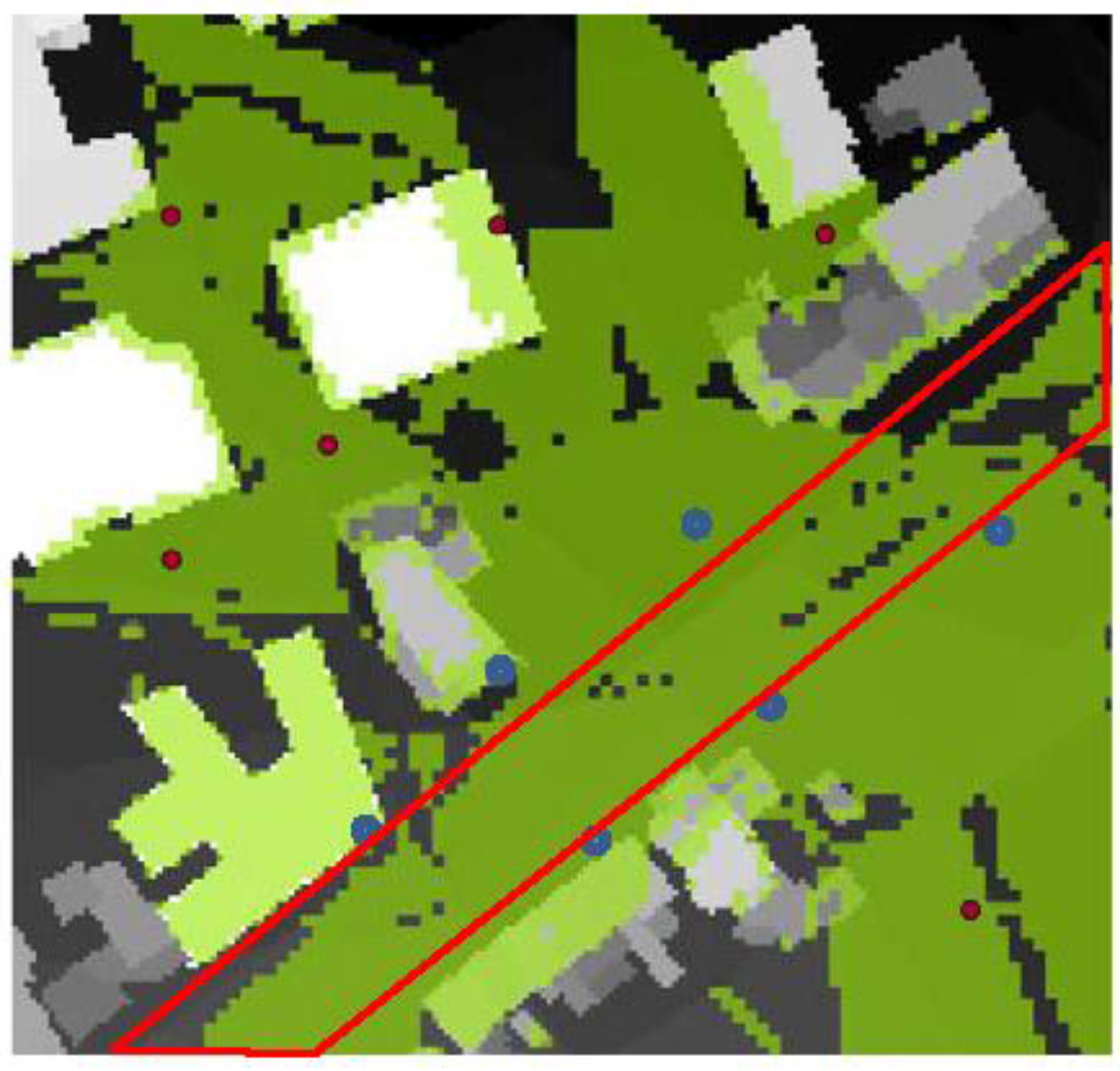
6.4. Optimization Considering the Environment Activities as CI

Sensor placement in an environment with a critical asset is the next thematic CI that is added to the knowledgebase of the context-aware algorithm. Assume a critical asset to be monitored for preventing any undesired access with a slight activity in its environment $\mathrm{\Xi }$, which is located beside a street with a high level of activities. Thus, the sensor movement rules need to be modified regarding to the interest of monitoring any intrusions within the fenced area, while sensor should not be always activated due to the traffic or other activity on the street. In this case, two types of weight maps are defined: (1) w_activity, which is the weight corresponding to the degree of activities in the environment; and (2) w_dc, that is the desirability of coverage weight with respect to the area that should be monitored. Obviously, the area with high amount of activities takes higher w_activity, and the desirable area supposed to be covered gets a higher w_dc. Let C_i be the circular coverage region of sensor s_i centered at the position p_i, then the score value of all possible positions p_i is:

$$scor{e}_{actdc}(p_i)=\left({\displaystyle \sum _{p_j\in C_i}{w}_{dc}(p_j)}\right)-\left({\displaystyle \sum _{p_j\in C_i}{w}_{activity}(p_j)}\right)$$

(10)

Similar to Section 6.3, the direction of sensor move is toward the farthest Voronoi vertex, and the stop point is at the position with the maximum score_actdc (new movement rule).

$${s^{\prime }}_i=\underset{p_i\in \overline{L_i}}{\arg \max }(scor{e}_{actdc}(p_i))$$

(11)

The reasoning engine also checks all previous CI, such as object elevations (used to define obstacles and visibility) and restricted areas, which were provided in the form of different weighted maps, in addition to the new situation. It means for each pixel, there are different values related to previous extracted CI, plus the new value (score) related to the environment activity.

To evaluate this case study, Zone 3 was defined as a region with high desirability of coverage including low activity, which is located beside Zone 1, which is a street, containing high activity and low interest of being covered (Figure 24). Both Zones 1 and 3 are unauthorized zones for installing sensors. The same as the previous case, the algorithm was run over 12 sensors with similar initial conditions. Figure 24 has the final sensor positions and the covered regions. Compared to the case of considering the street as the desirable area to be covered (Figure 22), in which six sensors were moved to cover the street, in this case three sensors were configured by the local context-aware optimization algorithm on the proper locations to cover Zone 3 (blue dots on Figure 24). Accordingly, the coverage over the street may be decreased while all surface of Zone 3 is covered. In this case study, the overall coverage is 55.72%, which is lower that other cases. It shows the importance of sensor configuration to cover a special place on the study area and of avoiding deploying sensors in an area with high activity but low interest of being covered.

Figure 24. Coverage map of deploying 12 sensors using the context-aware method, considering the activity in the network; Zone 3: the area with low activity, but high interested to be covered.

Figure 24. Coverage map of deploying 12 sensors using the context-aware method, considering the activity in the network; Zone 3: the area with low activity, but high interested to be covered.

7. Discussions and Conclusions

A local context-aware optimization method for sensor network deployment has been proposed in this paper, which considers the local information from the environment and the relevant information on the network. The main objective of the paper was to propose a more realistic context-aware deployment algorithm for sensor networks in a given environment. As mentioned in Section 1 and Section 2, integrating local information and relations of the network and surrounding environment helps to conduct an efficient sensor network deployment. Some instances of such information include adjacency relations, sensors configurations, obstacles that are blocking the line-of-sight, and the information about the physical environment elements. Accordingly, the concept of context was investigated and expanded for sensor network deployment. The CI then was categorized to three categories of spatial, temporal, and thematic to be clearly involved in sensor deployment. The mentioned investigations led authors to propose a flexible conceptual framework to handle sensor placement using Voronoi diagram and contextual information. Based on the proposed conceptual framework, a novel local context-aware optimization algorithm was developed. The proposed algorithm does not depend on the oversimplification of assumptions as is usually observed in other existing optimization algorithms. The novelty of our algorithm lies in explicit consideration of the local CI, such as environmental information, spatial locations, sensor adjacencies in the network, thematic and legal information for sensor placement, and sensors temporal configuration. Despite the capacity of the proposed algorithm to consider complex CI, it is simple and easy to implement. In addition, it used a flexible methodology that can accommodate all relevant information that would influence sensor placement. Thus, the proposed approach can address different sensor configurations under different circumstances or different environmental CI and sensor parameters. Consequently, if there are any changes in sensor parameters or environment, the optimization algorithm can simply take in the new relevant CI and regenerate a new sensor placement design adapted to the new situation.

In order to validate the proposed algorithm we have conducted several experiments. First, the results of the local context-aware algorithm were compared with a well-known global optimization algorithm (CMA-ES) in one case. The comparison shows almost the same percentage of final coverage value over the study area for both methods, while the computation required by the proposed local approach is significantly less than the global method. The local context-aware approach uses the local CI and spatial relations to perform the optimization. It explicitly considers the physical reality of the environment, instead of using the probabilistic information, which is generally used in global non-context-aware methods.

The developed algorithm was evaluated over many relevant case studies for performance with different application needs. In order to avoid the impact of different initial positions on the final outputs, the same initial conditions were applied at the starting point of optimization. Elevation and viewshed information were the first level of CI used in the local approach. For the next case study, some restricted areas were introduced to the algorithm. Given this CI, the optimization algorithm analyzed sensor displacement in the network and appropriate actions were determined. Another investigation was made to find how many sensors would be enough to cover the whole study area. It was conducted by increasing the number of sensors and its positive impact on the coverage. To analyze the capacity of the context-aware method in more complex situations, the desirability of coverage was added as supplementary CI. Environmental activities such as monitoring an environment with a slight activity containing a critical asset for preventing any undesired access located beside a street with a high level of activities were considered as the last part of the investigation over various CI case studies. In that step, regions with high activity and low desire of coverage were introduced to the algorithm. The extended algorithm was adapted to cover the desired region without being affected by the attraction of high activities of the surrounding regions. These inquiries illustrate how the proposed local context-aware algorithm is efficient in performing a sensor deployment optimization considering environmental and network CI.

The presented approach is a context-aware automated sensor deployment optimization method based on environmental and network information. A specialized context-aware process was introduced to exploit complex environmental information. The algorithm maximizes the performance whereas the processing time is minimized based on an optimal number of sensor displacements in the network. In addition, the proposed method profited from a local refinement of deployment using a deterministic solution, which avoids applying the stochastic black box methods.

References

1. Aziz, N.; Aziz, K.; Ismail, W. Coverage strategies for wireless sensor networks. World Acad. Sci. Eng. Technol. 2009, 50, 145–150. [Google Scholar]
2. Ahmed, N.; Kanhere, S.; Jha, S. The holes problem in wireless sensor networks: A survey. ACM SIGMOBILE Mob. Comput. Commun. Rev. 2005, 1, 1–14. [Google Scholar] [CrossRef]
3. Ghosh, A.; Das, S.K. Coverage and connectivity issues in wireless sensor networks: A survey. Pervasive Mob. Comput. 2008, 4, 303–334. [Google Scholar] [CrossRef]
4. Huang, C.; Tseng, Y. A survey of solutions to the coverage problems in wireless sensor networks. J. Internet Technol. 2005, 1, 1–9. [Google Scholar]
5. Megerian, S.; Koushanfar, F.; Potkonjak, M.; Srivastava, M.B. Worst and best-case coverage in sensor networks. IEEE Trans. Mob. Comput. 2005, 4, 84–92. [Google Scholar] [CrossRef]
6. Meguerdichian, S.; Koushanfar, F.; Potkonjak, M.; Srivastava, M.B. Coverage problems in wireless ad-hoc sensor networks. In Proceedings of the Twentieth Annual Joint Conference of the IEEE Computer and Communications Society (IEEE INFOCOM 2001), Anchorage, AK, USA, 22–26 April 2001; Volume 3, pp. 1380–1387.
7. Loscrí, V.; Natalizio, E.; Guerriero, F.; Mitton, N. Efficient coverage for grid-based mobile wireless sensor networks. In Proceedings of the 11th ACM Symposium on Performance Evaluation of Wireless Ad Hoc, Sensor, and Ubiquitous Networks (PE-WASUN’14), Montreal, QC, Canada, 21–26 September 2014.
8. Urrutia, J. Art Galleries and Illumination Problems. In Handbook on Computational Geometry; Elsevier Sciences Publisher: New York, NY, USA, 2000; Chapter 22; pp. 973–1026. [Google Scholar]
9. Gonzales-Banos, H.; Latombe, J.-C. A Randomized Art-Gallery Algorithm for Sensor Placement. In Proceedings of the Symposium on Computational Geometry (SCG 2001), Medford, MA, USA, 3–5 June 2001; pp. 232–240.
10. Wang, G.; Cao, G.; la Porta, T. Movement-assisted sensor deployment. IEEE Trans. Mob. Comput. 2006, 5, 640–652. [Google Scholar] [CrossRef]
11. Thai, M.T.; Wang, F.; Du, D.H.; Jia, X. Coverage problems in wireless sensor networks: Designs and analysis. Int. J. Sens. Netw. 2008, 3, 191–203. [Google Scholar] [CrossRef]
12. Cardei, M.; Wu, J. Coverage in Wireless Sensor Networks. PhD Thesis, Department of Computer Science and Engineering, Florida Atlantic University, Boca Raton, FL, USA, 2004. [Google Scholar]
13. Zou, Y.; Chakrabarty, K. Sensor deployment and target localization based on virtual forces. In Proceedings of the Twenty-Second Annual Joint Conference of the IEEE Computer and Communications, IEEE Societies, INFOCOM 2003, San Francisco, CA, USA, 30 March–3 April 2003; Volume 2.
14. Niewiadomska-Szynkiewicz, E.; Marks, M. Optimization Schemes For Wireless Sensor Network Localization. Int. J. Appl.Math. Comput. Sci. 2009, 19, 291–302. [Google Scholar] [CrossRef]
15. Romoozi, M.; Ebrahimpour-komleh, H. A Positioning Method in Wireless Sensor Networks Using Genetic Algorithms. In Proceedings of 2012 International Conference on Medical Physics and Biomedical Engineering (ICMPBE2012), Singapore, 12–14 September 2012; pp. 174–179.
16. Argany, M.; Mostafavi, M.A.; Karimipour, F.; Gagné, C. A GIS based wireless sensor network coverage estimation and optimization: A voronoi approach. Trans. Comput. Sci. XIV 2011, 6970, 151–172. [Google Scholar]
17. Argany, M.; Mostafavi, M.A.; Akbarzadeh, V.; Gagné, C.; Yaagoubi, R. Impact of the Quality of Spatial 3D City Models on Sensor Networks. Geomatica 2012, 66, 291–305. [Google Scholar] [CrossRef]
18. Akbarzadeh, V.; Gagne, C.; Parizeau, M.; Argany, M.; Mostafavi, M.A. Probabilistic Sensing Model for Sensor Placement Optimization Based on Line-of-Sight Coverage. IEEE Trans. Instrum. Meas. 2013, 62, 293–303. [Google Scholar] [CrossRef]
19. Erdelj, M.; Loscrí, V.; Natalizio, E.; Razafindralambo, T. Multiple point of interest discovery and coverage with mobile wireless sensors. Ad Hoc Netw. 2013, 1, 2288–2300. [Google Scholar] [CrossRef]
20. Dey, A.; Abowd, G.; Salber, D. A Conceptual Framework and a Toolkit for Supporting the Rapid Prototyping of Context-Aware Applications. Hum.-Comput. Interact. 2001, 16, 97–166. [Google Scholar] [CrossRef]
21. Brown, P.; Bovey, J.; Chen, X. Context-Aware Applications: From the Laboratory to the Marketplace. Pers. Commun. 1997, 4, 58–64. [Google Scholar] [CrossRef]
22. Ryan, N.; Pascoe, J.; Morse, D. Enhanced Reality Fieldwork: The Context-Aware Archaeological Assistant. Bar Int. Ser. 1999, 750, 269–274. [Google Scholar]
23. Dey, A. Context-aware computing: The CyberDesk project. In Proceedings of the AAAI 1998 Spring Symposium on Intelligent Environments, Palo Alto, CA, USA, 23–25 March 1998; pp. 51–54.
24. Schilits, B.N.; Theimer, M.M. Disseminating Active Map Information to Mobile Hosts. IEEE Netw. 1994, 8, 22–32. [Google Scholar] [CrossRef]
25. Franklin, D.; Flaschbart, J. All gadget and no representation makes jack a dull environment. In Proceedings of the AAAI 1998 Spring Symposium on Intelligent Environment, Palo Alto, CA, USA, 23–25 March 1998; pp. 155–160.
26. Hull, R. Towards situated computing. In Proceeding of the 1st International Symposium on Wearable Computers, Boston, MA, USA, 13–14 October 1997; pp. 146–153.
27. Shermer, T. Recent results in art galleries. Proc. IEEE 1992, 80, 1384–1399. [Google Scholar] [CrossRef]
28. Argany, M.; Mostafavi, M.A.; Karimipour, F. Voronoi-Based Approaches for Geosensor Networks Coverage Determination and Optimisation: A Survey. In Proceedings of the 2010 International Symposium on Voronoi Diagrams in Science and Engineering, Quebec, QC, Canada, 28–30 June 2010; pp. 115–123.
29. Fan, G.; Jin, S. Coverage Problem in Wireless Sensor Network: A Survey. J. Netw. 2010, 5, 1033–1040. [Google Scholar] [CrossRef]
30. Wang, L.; Shen, H.; Chen, Z.; Lin, Y. Voronoi tessellation based rapid coverage decision algorithm for wireless sensor networks. In Proceedings of 4th International Conference on Ubiquitous Intelligence and Computing, Hong Kong, China, 11–13 July 2007; pp. 495–502.
31. Bai, X.; Lai, T.H. Deploying Wireless Sensors to Achieve Both Coverage. In Proceedings of the MobiHoc’06, Florence, Italy, 22–25 May 2006; pp. 131–142.