Towards Long-Term Multi-Hop WSN Deployments for Environmental Monitoring: An Experimental Network Evaluation †

 ,
,
Abstract
:1. Introduction
2. Related Works

| Testbed | Deployment Analysis Time | Size | Environment | Hardware Platform | Application Category |
|---|---|---|---|---|---|
| MoteLab [11] | N/A | 190 nodes | Indoors | TMote Sky | Application testing |
| Kansei Genie [5] | N/A | 700 nodes | Indoors | XSM, TelosB, Imote2 | Application testing |
| Indriya [12] | N/A | 139 nodes | Indoors | TelosB | Application testing |
| SensLab [13] | N/A | 256 × 4 nodes | Indoors | WSN430 | Application testing |
| FlockLab [14] | N/A | 30 × 4 nodes | Indoors | TinyNode, Opal, TelosB, IRIS | Application testing |
| VigilNet [15] | ~days | 70 nodes | Outdoors (open area) | Mica2 | Tracking/detection |
| Springbrook [4] | 7 days | 10 nodes | Outdoors (forested area) | Fleck-3 | Periodic sensing |
| ExScal [3] | 15 days | 1200 nodes | Outdoors (open area) | Mica2 (XSM) | Tracking/detection |
| GreenOrbs [6] | 29 days | 330 nodes | Outdoors (forest) | TelosB | Periodic sensing |
| SNF [16] | 30 days | 57 nodes | Outdoors (forest) | M2135 | Periodic sensing |
| Redwoods [17] | 44 days | 33 nodes | Outdoors (on a tree) | Mica2Dot | Periodic sensing |
| SensorScope [18] | 2 months | < 100 nodes (16 outdoor) | Outdoors (glacier) | TinyNode | Periodic sensing |
| Trio [2] | 4 months | 557 nodes | Outdoors (open area) | Trio Mote | Tracking/detection |
| GDI [19] | 4 months | 98 nodes | Outdoors | Mica2Dot | Periodic sensing |
| ASWP [20] | 1 year + 6 months | 42–52 nodes | Outdoors (forested area) | MicaZ, IRIS | Periodic sensing |
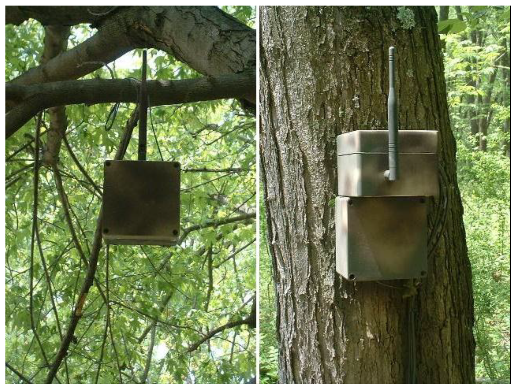
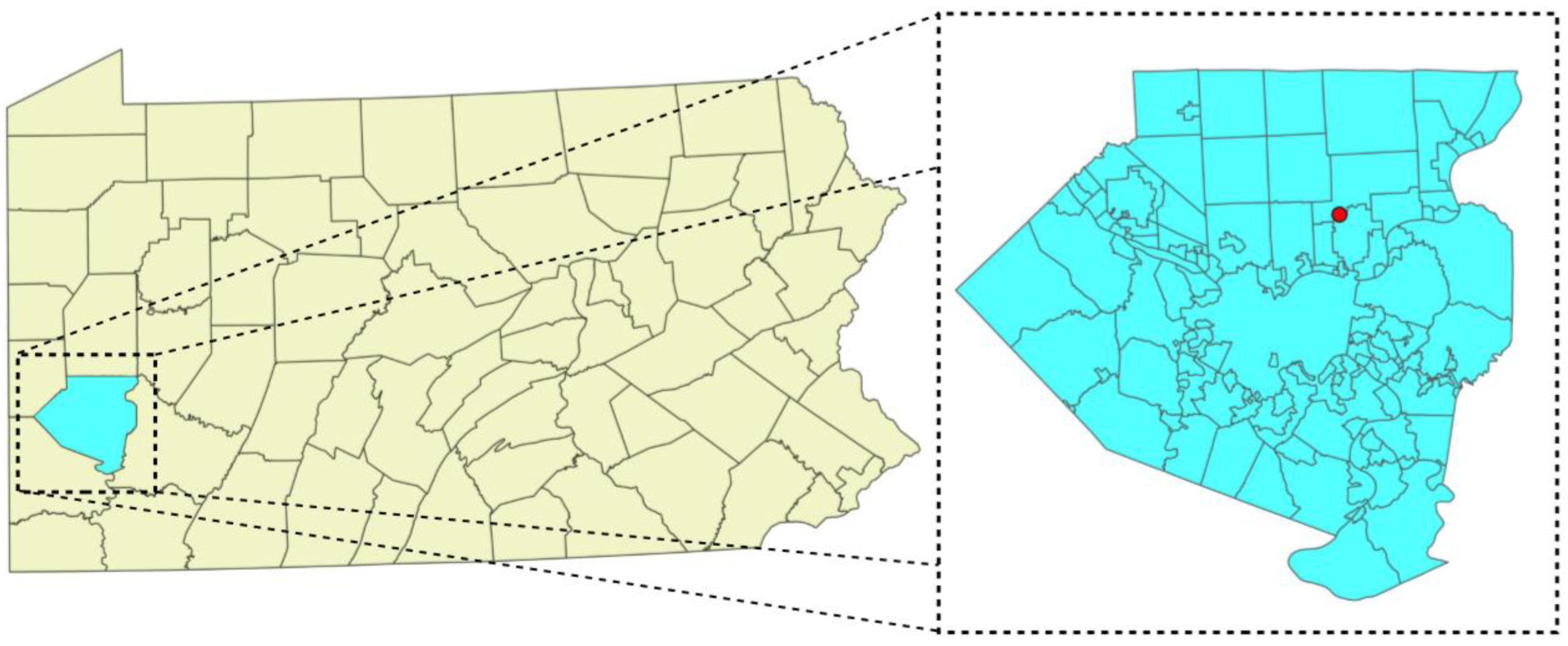
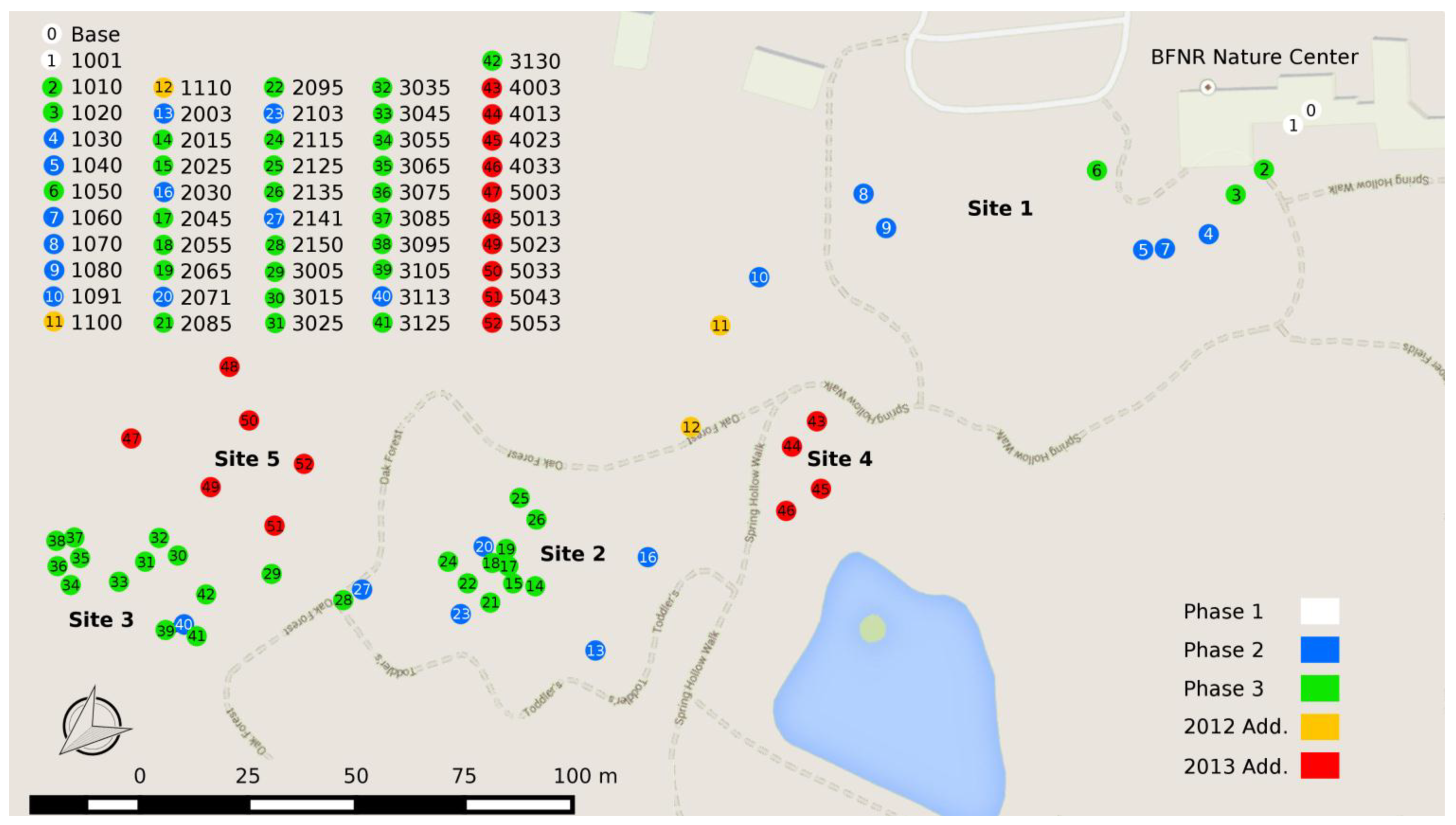
3. Testbed Deployment
3.1. Gateway and Data Management
3.2. Software Description
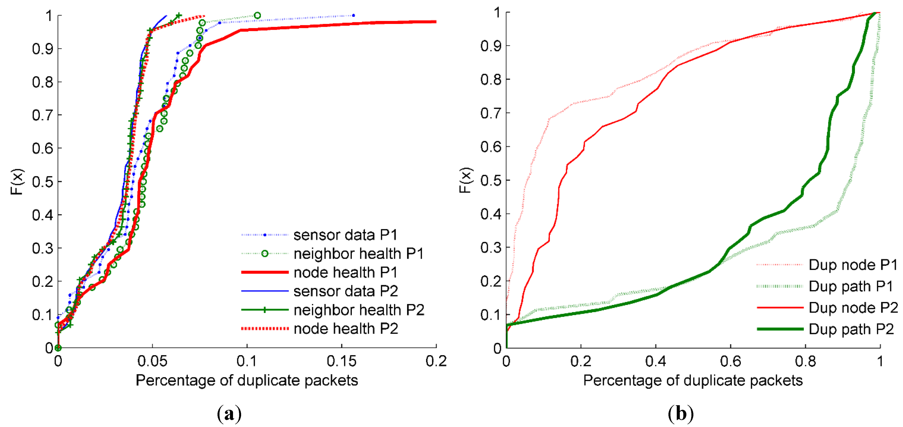
- Sensor data: correspond to the actual sensor readings of the motes and depends on the data acquisition board (MDA300, in this case). This packet type was configured with a sampling interval of 15 min.
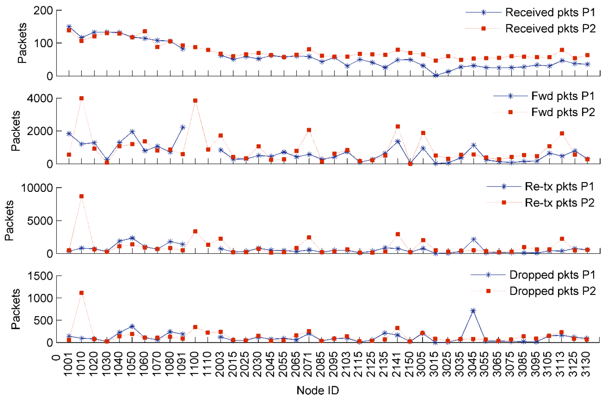
- Node health data: contain node-level statistics that include the following accumulated counters: node health data packets generated at the node, total number of packets generated at the node (including all three packet types), number of packets forwarded from other nodes, number of retransmissions, number of packets dropped at the node, path cost to the base station (e.g., node cost), and information about the link connecting to the parent node. Counters for node health data packets and node generated packets reflect unique packet identifiers from the point of view of the WSN application; therefore, they do not include packet retransmissions.
- Neighbor health data: report the information of up to five neighbor nodes including their link information and path cost values. Neighbor health packets and node health packets are sent alternatively, one type after the other, and they are defined with a single interval named Health Update Interval (HUI). The HUI is set by default to 10 min, thus the effective transmission for each health data type is twice the initial HUI: 20 min.
| Parameter | Value |
|---|---|
| Data sampling interval | 15 min |
| Initial data sampling interval | 1 min for the first 10 packets |
| Summary packet interval | 30 min |
| Radio channel | 26 |
| Transmission power | Maximum |
| Low-power-listening (LPL) sleep interval | 1 s |
| Maximum CTP retransmissions | 7 attempts |
| Maximum Trickle timer interval | 1 h |
4. Network Performance
4.1. XMesh
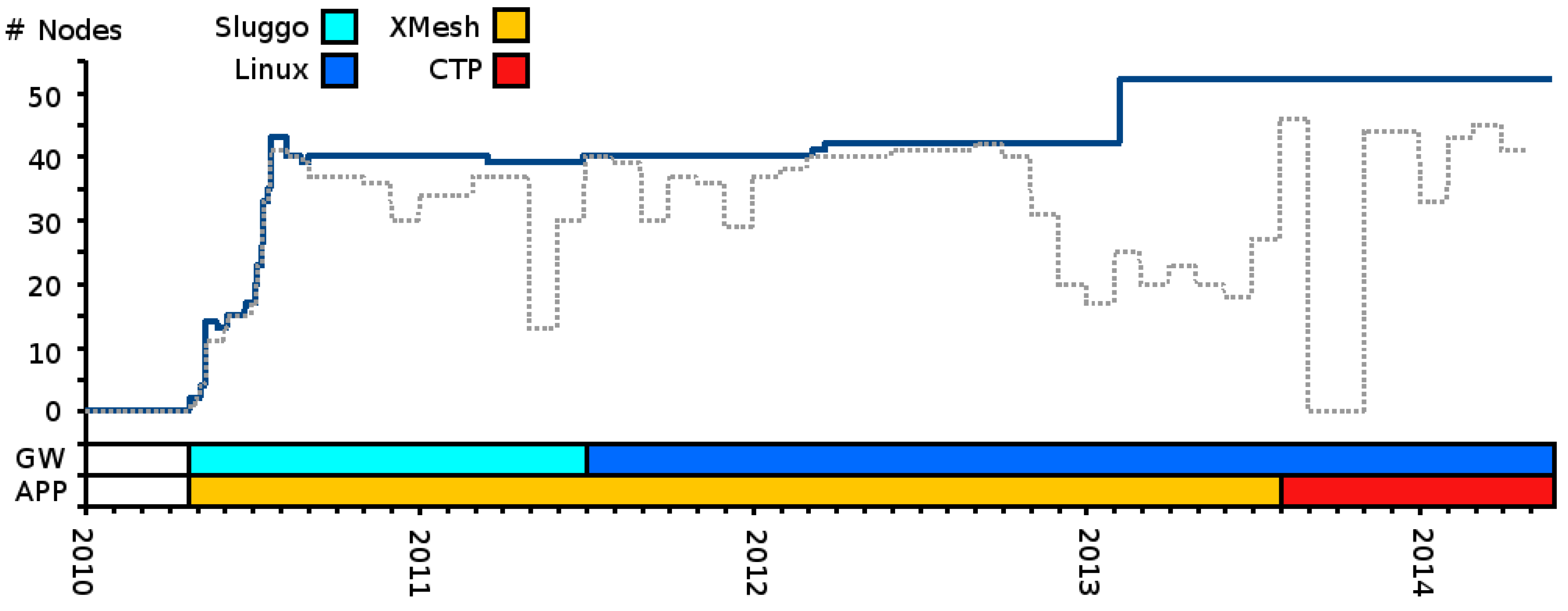
| Period | P1 | P1a | P2 | P2a | |
|---|---|---|---|---|---|
| Range | August 2011–February 2012 | 15 September 2011–20 October 2011 | March 2012–August 2012 | 1 July 2012–4 August 2012 | |
| Description | Before IRIS motes | Sub-period of P1 | After IRIS motes | Sub-period of P2 | |
| Deployed Nodes | 40 | 40 | 42 | 42 | |
| Daily Connected Nodes | Max. | 39 | 37 | 41 | 41 |
| Avg. | 24 | 22 | 34 | 36 | |
| Min. | 4 | 4 | 4 | 25 | |
| Algorithm 1: | Identifies and Removes Duplicate Packets |
| Input: | Packets from the same node ordered by time and marked as valid packets |
| Output: | Packets marked either as valid or duplicate |
| Begin While pkti = nextValidPacket() do loop on pkti While pkti is valid AND pktj = nextValidPacket() do loop on pktj If |pkti.time − pktj.time| < T − ∂T then // pktj is in the effective interval of pkti If pkti.content == pktj.content then // pkti and pktj have the same content Mark pktj as a duplicate of pkti End Else // pktj is on the next interval Break loop on pktj End End pkti = nextValidPacket() End // end loop on pkti End | |
| Period | Node Health Data Duplicate % (with Seq. Number) | Node Health Data Duplicate % (with Our Algorithm) | Sensor Data Duplicate % | Neighbor Health Data Duplicate % |
|---|---|---|---|---|
| P1 | 4.10% | 4.04% | 3.82% | 3.65% |
| P2 | 3.16% | 3.07% | 3.01% | 3.08% |

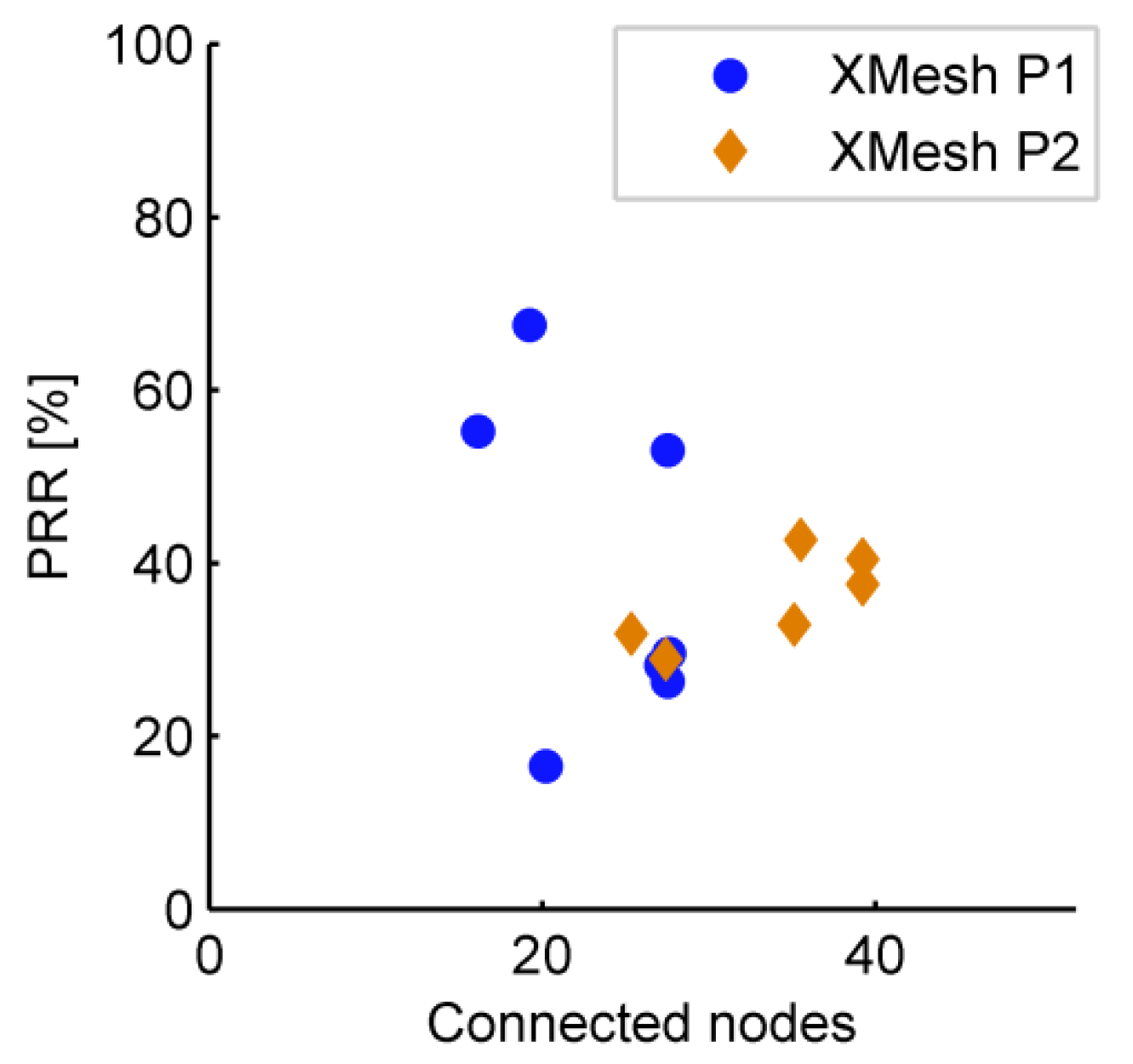
| Period | PRR | PSR |
|---|---|---|
| P1 | 35.17% | 49.09% |
| P1a | 61.04% | 53.92% |
| P2 | 36.01% | 46.08% |
| P2a | 42.16% | 45.33% |
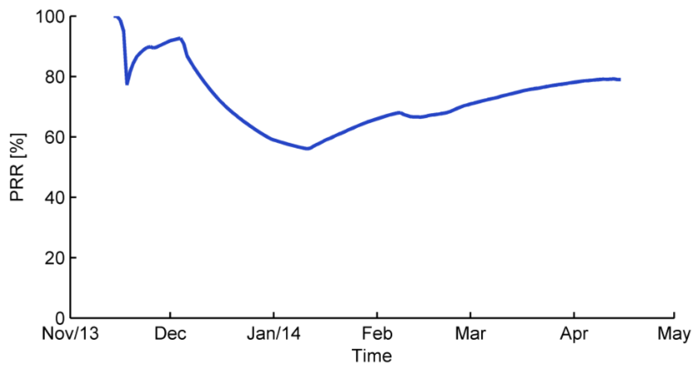
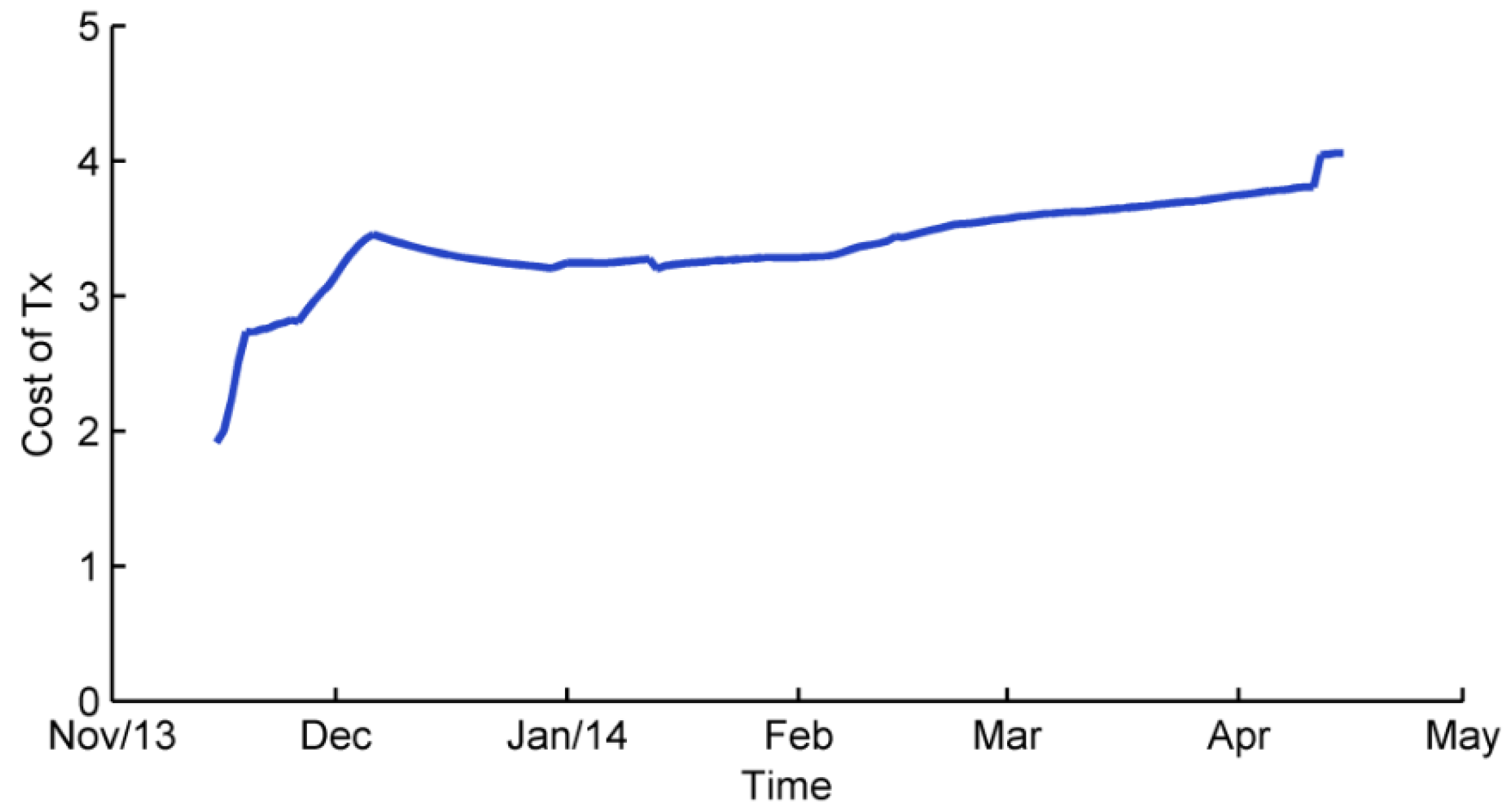
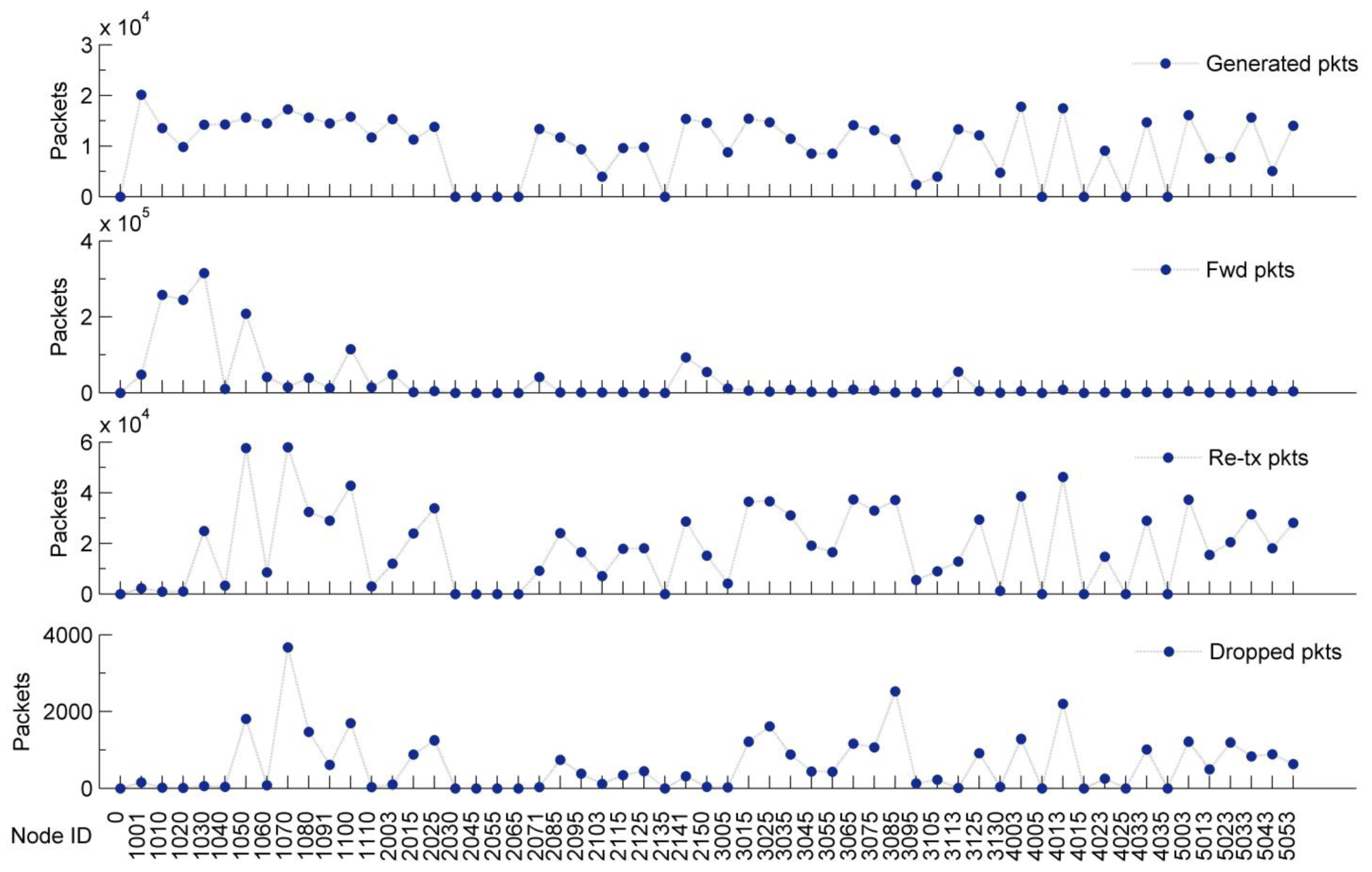
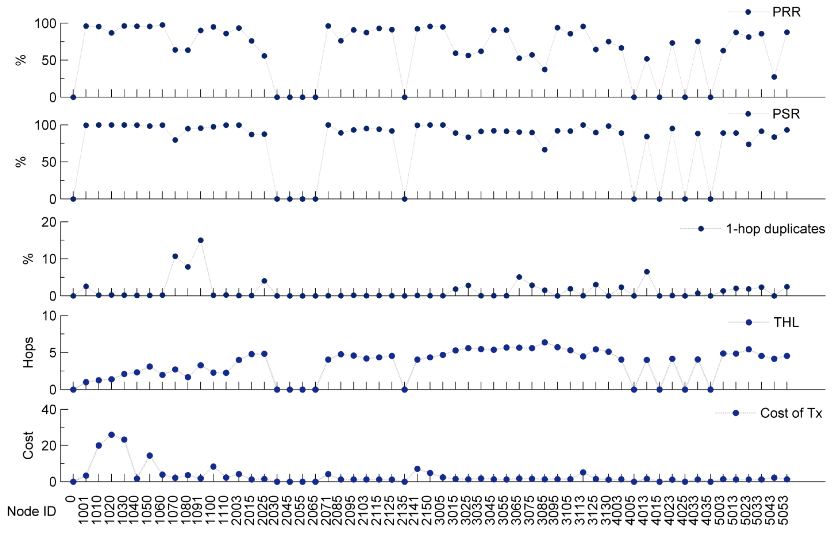
4.2. CTP


5. Network Costs
| Category | Total Cost | % |
|---|---|---|
| Deployment Costs | $31,500 | 52 |
| Labor Costs | $23,900 | 40 |
| Maintenance Costs | $5000 | 8 |
| Total | $60,400 | 100 |
5.1. Deployment Costs
| Category | Description | Cost |
|---|---|---|
| Hardware | Wireless motes, antennas, gateway, etc. | $15,940 |
| External Sensors | Soil moisture and sap flow. | $12,600 |
| Power | Batteries (AA, D, 12 V). | $1500 |
| Enclosures | Waterproof boxes, insulation and desiccants. | $1400 |
| Mounting | PVC pipe, wiring, nuts, bolts and screws. | $60 |
| Total | Cumulative cost. | $31,500 |
5.2. Labor Costs

| Category | Total Cost | Per Visit | % |
|---|---|---|---|
| Time Cost | $22,200 | $144 | 93 |
| Transportation | $1700 | $11 | 7 |
| Total | $23,900 | $155 | 100 |
5.3. Maintenance Costs
| Category | Total Cost | Per Visit | % |
|---|---|---|---|
| Hardware and Enclosures | $3700 | $24 | 74 |
| Power | $1300 | $8 | 26 |
| Total | $5000 | $32 | 100 |
5.4. Unforeseen Costs
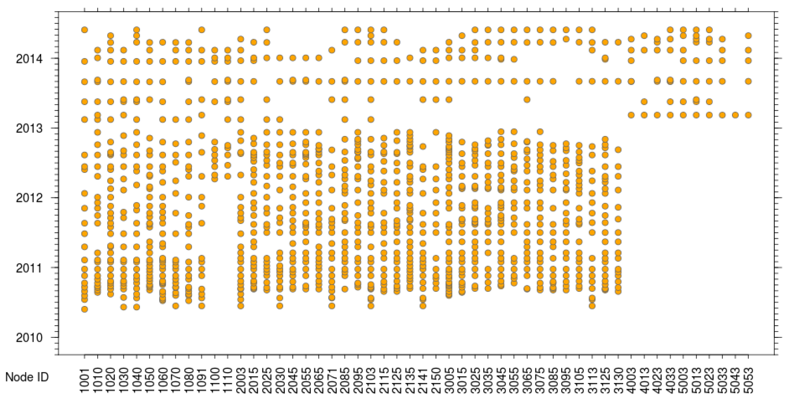
5.4.1. Node ID Change Phenomenon
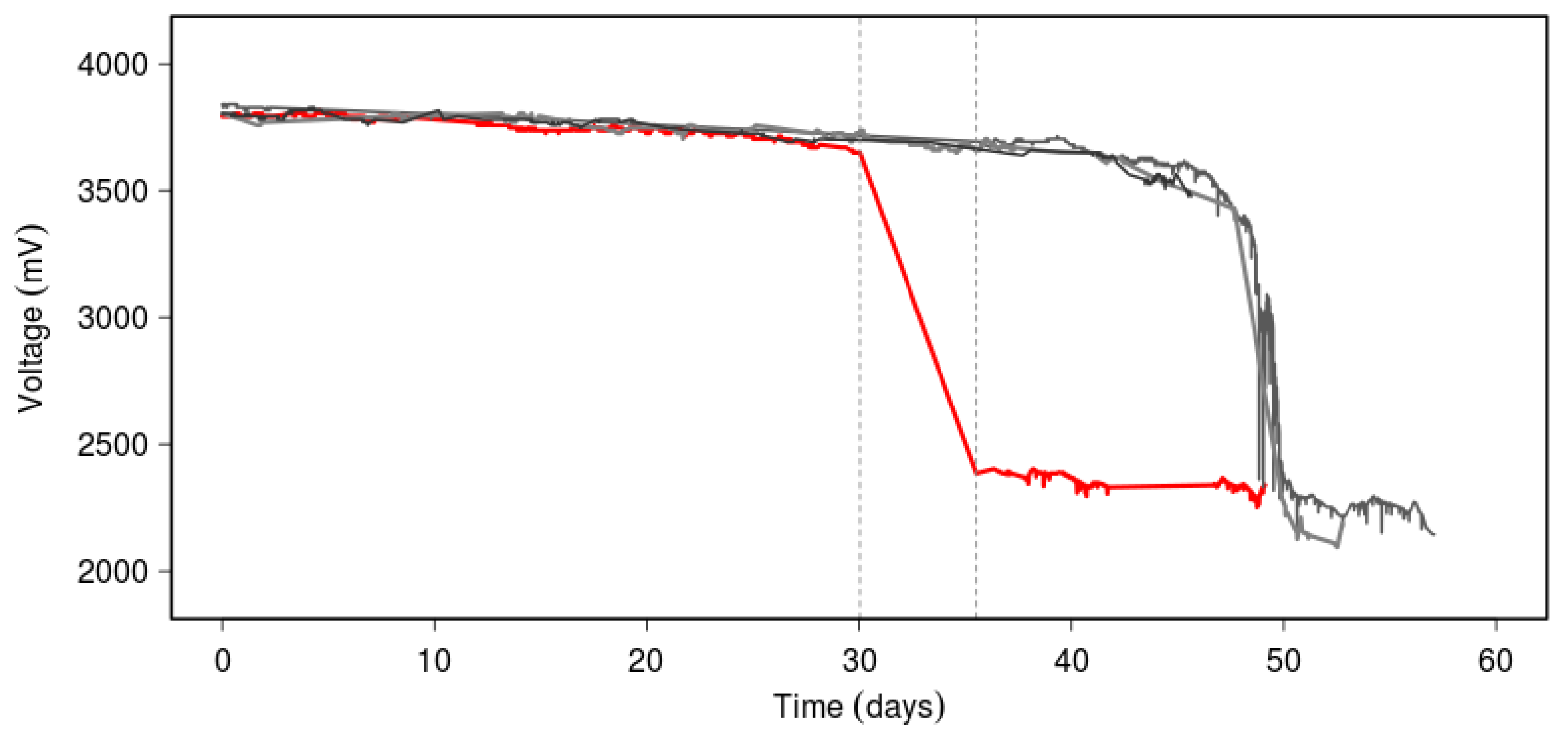
5.4.2. Network Outage Battery Loss

5.4.3. Internet Security
6. Conclusions
Acknowledgments
Author Contributions
Conflicts of Interest
References
- Akyildiz, I.F.; Su, W.; Sankarasubramaniam, Y.; Cayirci, E. Wireless sensor networks: A survey. Comput. Netw. 2002, 38, 393–422. [Google Scholar] [CrossRef]
- Dutta, P.; Hui, J.; Jeong, J.; Kim, S.; Sharp, C.; Taneja, J.; Tolle, G.; Whitehouse, K.; Culler, D. Trio: Enabling sustainable and scalable outdoor wireless sensor network deployments. In Proceedings of the 5th International Conference on Information Processing in Sensor Networks, Nashville, TN, USA, 19–21 April 2006; pp. 407–415.
- Bapat, S.; Kulathumani, V.; Arora, A. Analyzing the yield of exscal, a large-scale wireless sensor network experiment. In Proceedings of the 13th IEEE International Conference on Network Protocols (ICNP 2005), Boston, MA, USA, 6–9 November 2005; p. 10.
- Wark, T.; Hu, W.; Corke, P.; Hodge, J.; Keto, A.; Mackey, B.; Foley, G.; Sikka, P.; Brunig, M. Springbrook: Challenges in developing a long-term, rainforest wireless sensor network. In Proceedings of the International Conference on Intelligent Sensors, Sensor Networks and Information Processing (ISSNIP 2008), Sydney, Australia, 15–18 December 2008; pp. 599–604.
- Ertin, E.; Arora, A.; Ramnath, R.; Naik, V.; Bapat, S.; Kulathumani, V.; Sridharan, M.; Zhang, H.; Cao, H.; Nesterenko, M. Kansei: A testbed for sensing at scale. In Proceedings of the 5th International Conference on Information Processing in Sensor Networks, Nashville, TN, USA, 19–21 April 2006; pp. 399–406.
- Liu, Y.; He, Y.; Li, M.; Wang, J.; Liu, K.; Li, X. Does wireless sensor network scale? A measurement study on greenorbs. IEEE Trans. Parallel Distrib. Syst. 2013, 24, 1983–1993. [Google Scholar] [CrossRef]
- Gnawali, O.; Guibas, L.; Levis, P. A case for evaluating sensor network protocols concurrently. In Proceedings of the 5th ACM International Workshop on Wireless Network Testbeds, Experimental Evaluation and Characterization, Chicago, IL, USA, 20–24 September 2010; pp. 47–54.
- Puccinelli, D.; Gnawali, O.; Yoon, S.; Santini, S.; Colesanti, U.; Giordano, S.; Guibas, L. The impact of network topology on collection performance. In Wireless Sensor Networks; Springer: Bonn, Germany, 2011; pp. 17–32. [Google Scholar]
- MEMSIC. Micaz, wireless measurement system. Available online: http://www.memsic.com/userfiles/files/Datasheets/WSN/6020-0060-04-B_MICAz.pdf (accessed on 27 November 2014).
- Al-Karaki, J.N.; Kamal, A.E. Routing techniques in wireless sensor networks: A survey. IEEE Wirel. Commun. 2004, 11, 6–28. [Google Scholar] [CrossRef]
- Werner-Allen, G.; Swieskowski, P.; Welsh, M. Motelab: A wireless sensor network testbed. In Proceedings of the 4th International Symposium on Information Processing in Sensor Networks, Los Angeles, CA, USA, 25–27 April 2005; p. 68.
- Doddavenkatappa, M.; Chan, M.C.; Ananda, A.L. Indriya: A low-cost, 3D wireless sensor network testbed. In Testbeds and Research Infrastructure. Development of Networks and Communities; Springer: Shanghai, China, 2012; pp. 302–316. [Google Scholar]
- Des Rosiers, C.B.; Chelius, G.; Fleury, E.; Fraboulet, A.; Gallais, A.; Mitton, N.; Noël, T. Senslab very large scale open wireless sensor network testbed. In Proceedings of the 7th International ICST Conference on Testbeds and Research Infrastructures for the Development of Networks and Communities (TridentCOM), Shanghai, China, 17–19 April 2011.
- Lim, R.; Ferrari, F.; Zimmerling, M.; Walser, C.; Sommer, P.; Beutel, J. Flocklab: A testbed for distributed, synchronized tracing and profiling of wireless embedded systems. In Proceedings of the 12th International Conference on Information Processing in Sensor Networks, Philadelphia, PA, USA, 8–11 April 2013; pp. 153–166.
- He, T.; Krishnamurthy, S.; Luo, L.; Yan, T.; Gu, L.; Stoleru, R.; Zhou, G.; Cao, Q.; Vicaire, P.; Stankovic, J.A. Vigilnet: An integrated sensor network system for energy-efficient surveillance. ACM Trans. Sens. Netw. (TOSN) 2006, 2, 1–38. [Google Scholar] [CrossRef]
- Kerkez, B.; Glaser, S.D.; Bales, R.C.; Meadows, M.W. Design and performance of a wireless sensor network for catchment-scale snow and soil moisture measurements. Water Resour. Res. 2012, 48. [Google Scholar] [CrossRef]
- Tolle, G.; Polastre, J.; Szewczyk, R.; Culler, D.; Turner, N.; Tu, K.; Burgess, S.; Dawson, T.; Buonadonna, P.; Gay, D. A macroscope in the redwoods. In Proceedings of the 3rd International Conference on Embedded Networked Sensor Systems, San Diego, CA, USA, 2–4 November 2005; pp. 51–63.
- Barrenetxea, G.; Ingelrest, F.; Schaefer, G.; Vetterli, M.; Couach, O.; Parlange, M. Sensorscope: Out-of-the-box environmental monitoring. In Proceedings of the International Conference on Information Processing in Sensor Networks (IPSN’08), St. Louis, MI, USA, 22–24 April 2008; pp. 332–343.
- Szewczyk, R.; Mainwaring, A.; Polastre, J.; Anderson, J.; Culler, D. An analysis of a large scale habitat monitoring application. In Proceedings of the 2nd International Conference on Embedded Networked Sensor Systems, Baltimore, MD, USA, 3–5 November 2004; pp. 214–226.
- Navarro, M.; Davis, T.W.; Liang, Y.; Liang, X. A study of long-term wsn deployment for environmental monitoring. In Proceedings of the 2013 IEEE 24th International Symposium on Personal Indoor and Mobile Radio Communications (PIMRC), London, UK, 8–11 September 2013; pp. 2093–2097.
- NOAA National Climatic Data Center. Ranking of cities based on percentage annual possible sunshine. Available online: http://www1.ncdc.noaa.gov/pub/data/ccd-data/pctposrank.txt (accessed on 9 September 2014).
- Northeast Regional Climate Center (NRCC). Percent possible sunshine. Available online: http://www.nrcc.cornell.edu/ccd/pctpos.html (accessed on 9 September 2014).
- Cerpa, A.; Elson, J.; Estrin, D.; Girod, L.; Hamilton, M.; Zhao, J. Habitat monitoring: Application driver for wireless communications technology. ACM SIGCOMM Comput. Commun. Rev. 2001, 31, 20–41. [Google Scholar] [CrossRef]
- Liu, T.; Sadler, C.M.; Zhang, P.; Martonosi, M. Implementing software on resource-constrained mobile sensors: Experiences with impala and zebranet. In Proceedings of the 2nd International Conference on Mobile Systems, Applications, and Services, Boston, MA, USA, 6–9 June 2004; pp. 256–269.
- Arora, A.; Dutta, P.; Bapat, S.; Kulathumani, V.; Zhang, H.; Naik, V.; Mittal, V.; Cao, H.; Demirbas, M.; Gouda, M. A line in the sand: A wireless sensor network for target detection, classification, and tracking. Comput. Netw. 2004, 46, 605–634. [Google Scholar] [CrossRef]
- Trubilowicz, J.; Cai, K.; Weiler, M. Viability of motes for hydrological measurement. Water Resour. Res. 2009, 45. [Google Scholar] [CrossRef]
- Peres, E.; Fernandes, M.A.; Morais, R.; Cunha, C.R.; López, J.A.; Matos, S.R.; Ferreira, P.; Reis, M. An autonomous intelligent gateway infrastructure for in-field processing in precision viticulture. Comput. Electron. Agric. 2011, 78, 176–187. [Google Scholar] [CrossRef]
- Musaloiu-e, R.; Terzis, A.; Szlavecz, K.; Szalay, A.; Cogan, J.; Gray, J. Life under your feet: A wireless soil ecology sensor network. In Proceedings of the 3rd Workshop on Embedded Networked Sensors (EmNets 2006), Cambridge, MA, USA, 30–31 May 2006.
- Matese, A.; Vaccari, F.P.; Tomasi, D.; Di Gennaro, S.F.; Primicerio, J.; Sabatini, F.; Guidoni, S. Crossvit: Enhancing canopy monitoring management practices in viticulture. Sensors 2013, 13, 7652–7667. [Google Scholar] [CrossRef] [PubMed]
- Vellidis, G.; Tucker, M.; Perry, C.; Kvien, C.; Bednarz, C. A real-time wireless smart sensor array for scheduling irrigation. Comput. Electron. Agric. 2008, 61, 44–50. [Google Scholar] [CrossRef]
- Szewczyk, R.; Polastre, J.; Mainwaring, A.; Culler, D. Lessons from a sensor network expedition. In Wireless Sensor Networks; Springer: Berlin, Germany, 2004; pp. 307–322. [Google Scholar]
- Moteiv Corporation. Tmote sky: Low Power Wireless Sensor Module; Technical Report; Moteiv Corporation: Redwood, CA, USA, June 2006. [Google Scholar]
- MEMSIC. Mda300 data acquisition board. Available online: http://www.memsic.com/userfiles/files/Datasheets/WSN/6020-0052-04_a_mda300-t.pdf (accessed on 27 November 2014).
- MEMSIC. Iris, wireless measurement system. Available online: http://www.memsic.com/userfiles/files/Datasheets/WSN/6020-0124-01_B_IRIS.pdf (accessed on 27 November 2014).
- Navarro, M.; Li, Y.; Liang, Y. Energy profile for environmental monitoring wireless sensor networks. In Proceedings of the 2014 IEEE Colombian Conference on Communications and Computing (COLCOM), Bogotá, Columbia, 4–6 June 2014; pp. 1–6.
- Stajano, F.; Cvrcek, D.; Lewis, M. Steel, cast iron and concrete: Security engineering for real world wireless sensor networks. In Applied Cryptography and Network Security; Springer: Berlin, Germany, 2008; pp. 460–478. [Google Scholar]
- Davis, T.W.; Liang, X.; Navarro, M.; Bhatnagar, D.; Liang, Y. An experimental study of wsn power efficiency: Micaz networks with xmesh. Int. J. Dis. Sens. Netw. 2012, 2012. [Google Scholar] [CrossRef]
- Navarro, M.; Bhatnagar, D.; Liang, Y. An integrated network and data management system for heterogeneous wsns. In Proceedings of the 2011 IEEE 8th International Conference on Mobile Adhoc and Sensor Systems (MASS), Valencia, Spain, 17–22 October 2011; pp. 819–824.
- MEMSIC. Xmesh user manual. Revision A. Available online: http://www.memsic.com/userfiles/files/User-Manuals/xmesh-user-manual-7430-0108-02_a-t.pdf (accessed on 27 November 2014).
- MEMSIC. Moteview user manual. Revision D. Available online: http://www.memsic.com/userfiles/files/User-Manuals/moteview-users-manual.pdf (accessed on 27 November 2014).
- Gnawali, O.; Fonseca, R.; Jamieson, K.; Moss, D.; Levis, P. Collection tree protocol. In Proceedings of the 7th ACM Conference on Embedded Networked Sensor Systems, Berkeley, CA, USA, 4–6 November 2009; pp. 1–14.
- Gnawali, O.; Fonseca, R.; Jamieson, K.; Kazandjieva, M.; Moss, D.; Levis, P. Ctp: An efficient, robust, and reliable collection tree protocol for wireless sensor networks. ACM Trans. Sens. Netw. (TOSN) 2013, 10. [Google Scholar] [CrossRef]
- Ganti, R.K.; Jayachandran, P.; Luo, H.; Abdelzaher, T.F. Datalink streaming in wireless sensor networks. In Proceedings of the 4th International Conference on Embedded Networked Sensor Systems, Boulder, CO, USA, 31 October–3 November 2006; pp. 209–222.
© 2014 by the authors; licensee MDPI, Basel, Switzerland. This article is an open access article distributed under the terms and conditions of the Creative Commons Attribution license (http://creativecommons.org/licenses/by/4.0/).
Share and Cite
Navarro, M.; Davis, T.W.; Villalba, G.; Li, Y.; Zhong, X.; Erratt, N.; Liang, X.; Liang, Y. Towards Long-Term Multi-Hop WSN Deployments for Environmental Monitoring: An Experimental Network Evaluation. J. Sens. Actuator Netw. 2014, 3, 297-330. https://doi.org/10.3390/jsan3040297
Navarro M, Davis TW, Villalba G, Li Y, Zhong X, Erratt N, Liang X, Liang Y. Towards Long-Term Multi-Hop WSN Deployments for Environmental Monitoring: An Experimental Network Evaluation. Journal of Sensor and Actuator Networks. 2014; 3(4):297-330. https://doi.org/10.3390/jsan3040297
Chicago/Turabian StyleNavarro, Miguel, Tyler W. Davis, German Villalba, Yimei Li, Xiaoyang Zhong, Newlyn Erratt, Xu Liang, and Yao Liang. 2014. "Towards Long-Term Multi-Hop WSN Deployments for Environmental Monitoring: An Experimental Network Evaluation" Journal of Sensor and Actuator Networks 3, no. 4: 297-330. https://doi.org/10.3390/jsan3040297