Assessing the Influence of Spatio-Temporal Context for Next Place Prediction using Different Machine Learning Approaches

Abstract

For next place prediction, machine learning methods which incorporate contextual data are frequently used. However, previous studies often do not allow deriving generalizable methodological recommendations, since they use different datasets, methods for discretizing space, scales of prediction, prediction algorithms, and context data, and therefore lack comparability. Additionally, the cold start problem for new users is an issue. In this study, we predict next places based on one trajectory dataset but with systematically varying prediction algorithms, methods for space discretization, scales of prediction (based on a novel hierarchical approach), and incorporated context data. This allows to evaluate the relative influence of these factors on the overall prediction accuracy. Moreover, in order to tackle the cold start problem prevalent in recommender and prediction systems, we test the effect of training the predictor on all users instead of each individual one. We find that the prediction accuracy shows a varying dependency on the method of space discretization and the incorporated contextual factors at different spatial scales. Moreover, our user-independent approach reaches a prediction accuracy of around 75%, and is therefore an alternative to existing user-specific models. This research provides valuable insights into the individual and combinatory effects of model parameters and algorithms on the next place prediction accuracy. The results presented in this paper can be used to determine the influence of various contextual factors and to help researchers building more accurate prediction models. It is also a starting point for future work creating a comprehensive framework to guide the building of prediction models.

1. Introduction

In the past decades, our movement behaviour has been increasingly complex and individual. Each year, people cover larger distances to satisfy their personal and professional demands due to the availability of cheaper and faster transport options, better integration of information technology with transport systems, and an increased share of inter-personal connectivity not being based on physical distance but common interests, personal past, or family reasons [1,2,3]. As a result, our movement patterns have become more irregular in terms of visited places, chosen transport models, or the time intervals during which we travel. While this increased mobility represents a vital backbone of our modern society, it also poses challenges with regards to sustainable urban planning, public transport scheduling, and the integration of information technology with transport systems.

A potential chance for understanding our highly complex mobility behaviour is provided by modern information technology (IT). Our smartphones are usually equipped with GPS receivers, and therefore provide an unprecedented wealth of automatically recorded tracking data on a highly detailed level. While many previous studies analyzed mobility using either cell tower data from telephone companies (which has a much lower spatial tracking resolution) or data from smaller samples of people outfitted with GPS trackers [4], the new wealth of automatically and passively collected multidimensional data allows us to analyze human mobility on more fine-grained levels than ever before [5]. However, the sensors in modern smartphones are not restricted to measuring the location of a user by integrating location fixes from different sources such as GPS, WLAN fingerprinting or cell tower triangulation, but additionally collect acceleration measurements, compass heading, temperature readings, and other contextual data. Especially the recording of accelerometer data is a good source to identify the transport modes a person is currently using, as well as the performed activity [6,7,8]. These and other context data could, however, also be used for other purposes, such as movement prediction.

In fact, predicting certain aspects of our movement behaviour is important to numerous application and serves various purposes. One can predict movement on different levels [9]. On a very high level, mobility prediction is for example important to determine bottlenecks in transportation systems and plan appropriate transportation infrastructure [10], to provide operational guidance in disaster situations [11], or to detect potentially dangerous upcoming events [12]. On this level, prediction models mostly neglect individual moving entities, but model aggregated flows of people transitioning from one area to another, or along certain transportation corridors (such as roads, train lines, or between airports). On a lower level, it is the goal to predict which location, area or point of interest (POI) a person is likely to visit at some point in the future. Exemplary use cases for such prediction include location-based recommendation systems [13], which need to be able to timely inform someone about relevant upcoming offers or nearby POIs. With increasing autonomy of transport system, these models will likely gain further importance, as they can be used to redistribute resources based on the forecasted mobility demands in certain regions. This trend can already be observed today on taxi systems such as Uber of Lyft, which base their prices on a demand prediction as a financial instrument to balance demands and offers [14,15]. Other examples include buses on demand, which have been proposed for a while and were recently tested at various locations around the world [16,17]. On the lowest level, movement prediction aims to predict the exact paths people and vehicles will take on a very small scale, which is especially important for driver assistance systems to provide crash avoidance and efficient transportation.

In this work, we primarily focus on movement prediction on the middle level: User location recordings are aggregated into discrete places, and predictions are made about which place is likely to be visited next by the user, given her movement history (cf. [18,19,20,21]). While such a model can be used for a variety of purposes, our intended use case is a location based recommender system. Among others, there are two major challenges in this context: First, such systems often suffer from the cold start problem [22]. This commonly encountered problem in recommender and prediction systems describes the fact that due to a lack of available data for first-time users, the usefulness of the system’s recommendations is reduced for two main reasons: not only does the system not have information on the interests of the new users, but there is also no existing knowledge on the basis of which to predict their future destinations. As a potential approach to address this issue, the method proposed and tested in the course of this study involves training the model on the data of previous users, and slowly adapting to new users as more data becomes available. A second problem for next place prediction is represented by the fact that different application scenarios frequently require resulting predictions to be made at differing spatial scales. Thus, for instance, while for location based advertising (e.g., encouraging visitors to Zurich to eat at a certain restaurant), predicting next locations on the scale of a city might be sufficient, for others, such as predicting pedestrian flows within the central shopping district, results on a much finer resolution can be needed. For this reason, we propose a novel hierarchical approach for next place prediction, which enables to obtain results on different levels of scale based on one integrative prediction model. This allows to make predictions on a scale which is appropriate to the current use case, while eliminating the need for separate models.

Another motivation for this work is based on a lack of generalizable insights about the relative effect of different model aspects, such as the prediction algorithm, the scale of prediction, the incorporated context data, and the space discretization method on the prediction accuracy. This is due to the fact that there is currently a lack of studies which are comparable in the sense that they show some degree of overlap in terms of the used trajectory dataset or other key aspects. Thus, a main contribution of our work is the analysis of different modeling approaches, the prediction accuracy at different spatial resolutions (which we incorporate via our novel hierarchical model described earlier), and the influence of various spatio-temporal features on the prediction. We compare the performance of the resulting models to several baseline predictors to determine the accuracy gains that can be reached by applying machine learning methods to large datasets of accurate movement data. We find that depending on the spatial scale of the predicted places, either raster- or cluster-based approaches tend to yield a higher accuracy, and that spatial and temporal context features differ in their effect at different spatial resolutions as well. We also find that the proposed model achieves a prediction accuracy of around 75%, which demonstrates its suitability to user-specific models, as well as its considerably better performance compared to the baseline predictors.

In the following Section 2, we will provide a review of previous research on mobility prediction, with a particular focus on research using similar modeling approaches than our work as well as comparably sized data sources. Section 3 introduces our hierarchical method, and its clustering, feature extraction, and prediction parts. In Section 4 we present the results of applying the model to a dataset of 41 users which were tracked over a time span of six months in Switzerland. In this section, the focus will be put on assessing the influence of various model parameters, spatial and temporal resolutions, as well as the different features chosen on the prediction accuracy. Finally, in Section 5 we discuss the findings before we highlight potential avenues for future research in Section 6.

2. Background

In this section, prior work of relevance for this study is presented. First, we focus on the particularities, applications and common challenges when mining movement trajectory datasets, especially when contextual information is included. Then, the scope is narrowed to the specific topic of predicting the next places of a moving person with a variety of algorithms.

2.1. Trajectory Data Mining and Context

When moving, people change their physical position within the reference system of geographic space [23], a fact which can be detected by means of various sensors including Global Navigation Satellite Systems (GNSS), Wireless Local Area Networks (WLAN), and many more [24]. The resulting data usually consist of trajectories, paths which describe the movement as a mapping function between space and time, and can be modelled as a series of chronologically ordered x, y-coordinate pairs enriched with a time stamp [5,23]. Mainly due to the fact that modern smart phones are typically equipped with GPS-receivers, it is now relatively easy and cheap to track large numbers of people, and therefore produce massive trajectory data sets.

As a reaction to these developments, there is now an established set of methods available for trajectory data mining (recent reviews are provided by [25] or [5]), which serves for extracting knowledge to either describe the moving entity’s observable behavior (e.g., [26]), or to predict its future activities (e.g., [27]). Despite this methodological progress, however, some critical research is still lacking. Thus, the prevalent context-independent view on trajectories has been termed one of the major pitfalls of movement data analysis [28]. Although our movement is always set in and influenced by its spatio-temporal context, which can involve the underlying physical space, the location of important places, the time, static or dynamic objects, and temporal events [29], the vast majority of work on trajectory data mining has so far focused on analyzing the geometry of the trajectories, while ignoring their contextual setting [30]. Notable examples include [31], who enrich pedestrian trajectories with information about the underlying urban infrastructure [32], who propose a framework for movement and context data integration [33], who annotate trajectories with points of interest (POIs) to identify significant places and movement patterns of people, or [29], who propose an event-based conceptual model for context-aware movement analysis based on spatio-temporal relations between movement events and the context. A further type of context which is particularly important when analyzing human movement is activity. Since the basic drive behind traveling is to perform activities at certain locations (although depending on the perspective, sometimes travel as such is also seen as activity), and activities are generally constrained by space and time (e.g., the location of shops and their opening times), incorporation of such restrictions into movement data analysis (and especially next place prediction) can increase the realism of the resulting models [34,35]. With the notion of constraints, time geography provides a valuable conceptual basis for such tasks [36]. Modeling activity, however, is not a trivial task, which is mainly due to its dependence on spatio-temporal granularity and hierarchical, nested structure. Thus, Ref. [35], for instance, proposes a hierarchical approach to model activities at different granularities based on movement data, while [31] uses a hierarchical model of the action of walking to infer personalized infrastructural needs for pedestrians based on their trajectories.

There are various potential sources for context data, such as further sensors of a person’s smartphone which can provide data on acceleration, orientation or the magnetic field [18], external data such as the weather [37] or social media check-ins [38], or user-specific features such as work and home locations, entertainment places and other points of interest as derived from her movement history [33,39,40].

2.2. Next Place Prediction

An important task of trajectory data mining is next place prediction. The ability to infer from the present position and historical movements of a user her next visited location is beneficial for numerous applications, including crowd management, transportation planning and congestion prediction, place recommender systems or location-based services [41,42].

2.2.1. Methods for Next Place Prediction

Although in most cases, our decisions and the resulting spatial behavior are not random, but the result of more or less rational decision making [43], it is not clear to what degree it is predictable. Thus, for instance, Ref. [44], when examining mobile phone data of 45,000 users, find 93% potential predictability of human mobility behavior across all users. In particular, they analyze entropy to detect a potential lack of order and therefore lack of predictability in the data. Using tracking data from cell phone towers, the authors combine the empirically determined user entropy and Fano’s inequality (relates the average information lost in a noisy channel to the probability of the categorization error) to identify the potential average predictability level. Furthermore, when segmenting each week into 168 hourly intervals, they find that on average 70% of the time, the user’s most visited location during that time interval coincides with her actual location. This finding, however, highly depends on the analysis scale. Thus, for instance, since [44] work with cell phone data, they predict movement and visited places on a coarse level, which would be different for e.g., GPS data which represents movements on a much more detailed level. It is also interesting to note that the theoretically achievable predictability reaches its highest level between noon and 1 pm, 6 pm and 7 pm, and in the night when users are supposed to be at home.

In previous work, various methods have been proposed for next place prediction. One of the most common approaches is to use Markov chains, with places typically being represented as states, and the movement between those places as transitions. By counting each user’s transitions, it is possible to calculate transition probabilities and a transition matrix. Given the current place, the latter then allows to identify the most likely next destination. A typical approach would be to partition space into grid cells or roads into segments and use the cells or segments as the states of the Markov model. Ref. [45], for instance, use a hidden Markov model for predicting the next destination given data which only partially represents a trip. They test their model with movement data representing 25%, 50%, 75% and 90% of the trip, and achieve a prediction accuracy between 36.1% and up to 94.5%. A similar approach is used by [18], who, however, additionally incorporate context data including the acceleration, the magnetic field and the orientation as recorded by the smartphone sensors to detect the used mode of transport, which is additionally used as an input. Further, [19] test the effect of varying the number of previously visited places which are taken into account for place prediction with a Markov model, and find that $n>2$ does not result in a substantial improvement. In general, work on predicting the next place of a person typically relies on historical movement data collected by this person exclusively (e.g., [18,19,45]). Further examples include [46], who use a person’s GPS trajectories to learn her personal map with significant places and routes, as well as predict next places and activities of a person, or [47], who use time, location and periodicity information, incorporated in the notion of spatiotemporal-periodic (STP) pattern, to predict next places for users exclusively based on their own pre-recorded data. A notable example is the study by [48], who use structured conditional random fields to model a person’s activities and places, and show that their model also performs sufficiently when being trained on other people’s movement data. Still, however, this study does not move beyond place detection and attempts no prediction of next places.

2.2.2. Neural Networks and Random Forests for Next Place Prediction

Recently, a number of studies have used random forests and neural networks for the task of next place prediction. Random forests, as described in [49], consist of multiple decision trees, which individually make their own prediction. If the desired labels are categorical, the final prediction of the forest is determined by majority voting. The advantages of the random forest method are that it is fast to train and provides the ability to deal with missing or unbalanced data. Besides, the essence of being an ensemble method makes random forest a strong classifier. Another big advantage of random forest is its convenience to calculate the feature importance in prediction [50]. Exemplary studies include [51], who use random forests for semantic obfuscation when predicting travel purposes, or [52], who predict users’ movements and app usage based on contextual information obtained from smartphone sensors.

In addition to random forest classifiers, neural networks (NN) are another commonly utilized method for next place prediction. The design of NN follows a simplified simulation of interconnected human brain cells. A typical NN consists of a dozen up to millions of artificial neurons arranged in a series of layers, where each neuron is connected to the others in the layers on both sides. During the training phase, the features are fed to the input layer, which will then be multiplied by the weight of each connection, passed through the hidden layers until reaching the output layer. The goal of the training process is to modulate the weights associated with each layer-layer connection. Usually, the number of output neurons corresponds to the number of target labels or classes. The output neuron with the highest probability will be the prediction result.

De Brébisson et al. [27] won the Kaggle taxi trajectory prediction challenge by designing a NN-based predictor which utilizes trajectory locations, start time, client ID, and taxi ID to perform next place prediction. Etter et al. [41] learn the users’ mobility histories to predict the next location based on the current context. Being one of the few studies which compare the performance of a range of methods, they find that among dynamical Bayesian networks, gradient boosted decision trees, and NN, the NN-based method performs best in terms of prediction accuracy. Liu et al. [22] propose a Spatial-Temporal Recurrent Neural Network (ST-RNN) to model local temporal and spatial contexts in each layer with time-specific transition matrices for different time intervals and distance-specific transition matrices for different geographical distances. Based on two typical datasets, their experimental results show significant improvements in comparison with other methods.

2.2.3. Summary: Research Needs for Next Place Prediction

In this background section, after a brief introduction to movement data mining and context in general, we presented an overview of the state of the art in the field of next place prediction with a particular emphasis on neural networks and random forests as potential methods for this purpose. Despite the wealth of related prior work, however, we can identify the following research needs which still have not been fully addressed:

• Although existing models achieve high accuracy when predicting a person’s next place, they rely on being trained on a set of pre-recorded movement trajectories of this particular person. As has been discussed, this drastically reduces their usefulness for new users, at least until a certain critical amount of data has been collected (cold start problem).
• In contrast to the existence of numerous approaches for next place prediction, it is still difficult to derive generalizable methodological recommendations for this task, e.g., with regards to modeling choices such as space discretization methods, machine learning algorithms or the list of integrated context features. This mainly results from a relative lack of comparability of the related studies.
• When predicting next places, available methods typically focus on a fixed scale of prediction, e.g., the country- (e.g., [45]), or city-level (e.g., [18,19]). In fact, however, for different application scenarios, next place predictions on different scales will be necessary. Instead of keeping separate models for these purposes, it would be desirable to be able to make predictions on different scales using one comprehensive model.

In this study, we address the first issue by using only one trajectory dataset but systematically vary selected model parameters to derive generalizable insights into their effects on the achieved accuracy and their mutual dependencies. The cold start problem is targeted by proposing and testing an approach to train the predictor on all users instead of each individual one. Finally, we propose a hierarchical prediction approach in order to use one model to obtain results on different levels of scale.

3. Method

The next place prediction method examined in this paper consists of three stages: place discretization, during which the continuous longitude and latitude variables are aggregated into discrete locations (where multiple longitude/latitude pairs can be mapped to the same location); feature extraction, which takes into account spatial and temporal context data and builds the input variables for the machine learning procedure; and next place prediction, in which step we use different machine learning methods to predict a future location for a user’s current position given the input variables.

3.1. Place Discretization

As a first step, the individual staypoints, i.e., all the points where a user stayed for at least a certain duration (e.g., home, work or shops), of the users must be mapped to discrete locations. For this, we test two different approaches, namely a raster-based and a cluster-based method. The first procedure involves rasterizing the study area into a set of regular raster cells and assigning the detected staypoints to the respective cell, is a computationally inexpensive form of place discretization, and a simple solution since every staypoint is assigned to exactly one raster cell. For the clustering alternative, we choose the k-means algorithm, which forms a set of k clusters by randomly choosing k longitude/latitude pairs and assigning each staypoint to the closest cluster. It then iteratively computes the centroid of all staypoints belonging to a cluster, and uses this longitude/latitude pair as the new cluster center. After again assigning each staypoint to the closest of the new clusters, the process is restarted by computing the centroid. Once the staypoint/cluster assignments do not change after an iteration, the k remaining clusters are output as final results.

There are strengths as well as drawbacks related to both approaches: For instance, a raster-based approach contains numerous cells with zero or only a few user locations (due to the fact that human movement is not uniformly distributed), whereas a cluster-based method always only yields areas that people actually visited at some point throughout their movement history. Thus, in the first case, a large number of potentially inaccessible and therefore irrelevant places are stored and analyzed, while in the second case, it is only possible to predict areas if at least one person has visited them before. This is especially problematic if the data gets frequently updated (as new staypoints are likely to be outside of existing clusters, and therefore at each update require a re-computation of the clusters), or if the model is to be applied to users without any previous data (as these would not have any clusters).

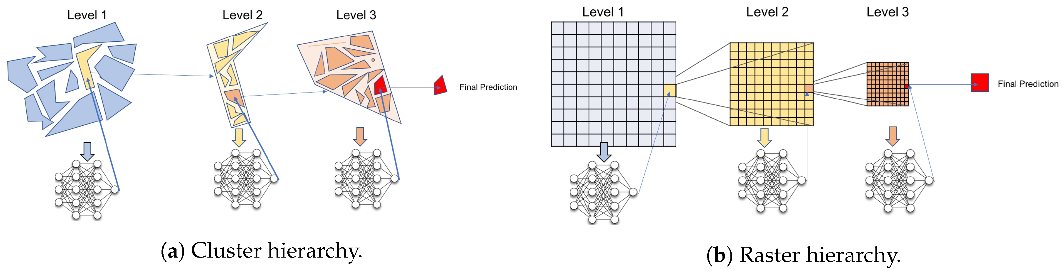
The prediction accuracy of human mobility highly depends on the analytical scale. Thus, for instance, if we predict movement on a global or continental scale, people will remain at approximately the same location throughout the year. On the city-level, in contrast, several locations will be visited for their everyday work-, errand- or leisure-related activities. For this reason, we aim to test the effect of multiple scale levels on the achieved prediction accuracy. At the same time, however, as mentioned previously, a simultaneous prediction of next locations on various scales can be a desirable capability of a prediction model, e.g., to be able to make location recommendations on corresponding scales or for different transportation planning applications. Here, it would be desirable to avoid the need for separate models for each prediction scale. For these reasons, we deploy a hierarchical approach for both the raster-based as well as the cluster-based models. For this approach, a practical challenge is to identify the appropriate number of prediction levels as well as suitable scales. In general, one could think of two possible methods to address this task: On the one hand, one could use a machine learning approach to identify these levels, e.g., gradually changing the predictive scales and optimizing for the achieved accuracy. A different approach would be to base this decision on expert opinion, i.e., implement a domain specialist’s recommendations with regards to the application scenarios expected to be addressed by our model. In the context of this study, we choose the latter approach, and define our three hierarchical level as follows: On the highest level, space is divided into segments of about 50 × 50 km cells. On the medium level, one cell is around 5 × 5 km large, and on the lowest level merely about 500 × 500 m. With regards to the cluster-based solution, we compute 100 clusters ($k=100$) on the highest scale level, and gradually refine it by clustering the locations within each of the 100 highest-level clusters into 30 smaller ones ($k=30$) and repeat this process with the resulting clusters in order to achieve a comparable increment of scale for the two space discretization approaches. Figure 1 illustrates both approaches. We choose these specific levels with regards to the aim of this study, namely to test a broad variety of settings (including scales of prediction). Potential application scenarios or business cases exist for all levels, thus, for instance, predictions at the coarsest level could be used to predict the demand for inter-regional train travels or tourist travel patterns, the medium level would be interesting for city-level location based advertising, while the finest level would allow for predicting travel flows to and from the city center. Please note, however, that for other application scenarios, both the number and scale of the levels could easily be adapted (e.g., for having an even finer resolution at the lowest level).

Furthermore, on the lowest level of scale, it is possible to identify an exact longitude/latitude pair of the next location in addition to predicting solely the (coarser) cluster or cell id. For this, the centroid of the set of locations visited by a single user within a cluster is computed (this stands in contrast to the place discretization process, where the data of all users is used). The motivation for this step is twofold: First, exact location prediction is valuable for many applications which require a more fine-grained prediction than on a 500 × 500 m raster (e.g., transport mode suggestions or location-based recommendations). Second, users are likely going to visit the same places they already visited before, yet seldom share their history of previously visited locations with other users. For this reason, an exact location prediction should consider only previously visited locations of a single user. We analyze the effect of such an exact location prediction with regards to accuracy.

3.2. Cluster and Raster Feature Extraction

We aim to predict the next likely location for a user based on:

• the spatial context of her current movement situation (user context)
• the visiting context of each location (location context)

Thus, for each trackpoint (a single GPS recording) of our movement dataset, we assess the current movement situation based on selected spatial attributes (including azimuth, distance to locations, etc.) of the user as well as selected (mostly temporal) aspects of the visiting context of locations (including visiting frequencies at the time of day and day of the week etc.) based on all users. For the latter, of course, the detected staypoints must be assigned to their respective label (i.e., their corresponding cluster or raster cell) first, to allow for a set of temporal features to be computed.

Table 1. Different machine learning input features extracted from the user location histories. The baseline methods are derived from these features by building a model that always predicts the location with the highest feature count. In the table, the number of locations is denoted as $n_l$.

Feature	Description	Baseline	Context Type
Three Hour Window ($h3$)	Counts the number of times any user visited a location in a $[-1,2]$ window (e.g., a time span from 13:00 to 16:00 when looking at 14:00) around each hour of the day ($24·n_l$ features). This captures hourly temporal patterns for individual regions.	Most visited location in a three hour window	location context (temporal)
Day of the Week ($dow$)	Counts the number a of times a location was visited on a certain day ($7·n_l$ features). This captures weekly temporal patterns for individual regions.	Most visited location on day x of the week	location context (temporal)
Week or Weekend ($week$)	Counts the number of times a location was visited during the week resp. on the weekend ($2·n_l$ features).	Most visited location on weekdays/weekends	location context (temporal)
Total Count ($tot$)	Counts the number of times a location was visited in total ($n_l$ features). This is important as often the location with the highest number of visits is the most likely next location.	Most visited location	location context
Distance ($dist$)	For each location in a user’s history, the distance to all clusters resp. raster cells is computed ($n_l$ features for each user trackpoint).	Nearest location	user context (spatial)
Azimuth ($azim$)	Computes the azimuth of a user’s current movement (the average over all previous trackpoints on the trajectory) to the location under examination ($n_l$ features for each user trackpoint).	-	user context (spatial)
Similar Routes ($act$)	Looking at similar routes of a user (that lie within 100 m and where the average direction deviates less than 90${}^{\circ }$), the number of ending location for each similar route is summed up ($n_l$ features for each user trackpoint).	Most visited location (of all endpoints of similar routes)	user context (spatial)

provides an overview of the different features for both types of context used within this analysis, and describes their computation in more detail. In the following, these serve as input for the prediction algorithm (based on the assumption that human mobility follows certain regular spatial and temporal movement patterns) which aims to learn implicit spatial and spatio-temporal dependencies between places and user movements.

The entire set comprises $34·n_l$ location-centered features which are static for all users ($h3$, $dow$, $week$, $tot$) and $3·n_l$ user-based features which need to be recomputed for each user position ($dist$, $azim$, $act$). In addition, for each step of the learning process the cluster label of the previous hierarchical step is used as an input for the machine learning model. In essence, this results in the following input vector $\overrightarrow{f_{h,i}}$ (for trackpoint i, and on hierarchy level h) and output label l (note that all features themselves are vectors and should be replaced by the individual elements in the formula below):

$$\overrightarrow{f_{h,i}}={(h3,dow,week,tot,dis{t}_i,azi{m}_i,ac{t}_i,l_{h-1})}^T$$

(1)

$$l=l_h$$

(2)

In this formula, $dis{t}_i$, $azi{m}_i$ and $ac{t}_i$ denote the user context feature at the current position i (cf. Table 1), $l_{h-1,i}$ denotes the cluster id on hierarchy level $h-1$ (this is of course only available for levels two and three), and $l=l_h$ is the predictor output on the current hierarchy level. The machine learning algorithm then uses the generated training data to approximate the function $\overrightarrow{f_{h,i}}\mapsto l$ in the best possible way.

3.3. Next Place Prediction

We deploy and analyze two different machine learning methods in this paper, starting with a feed-forward neural network (NN) with two hidden layers. Since the input data is not linearly separable, at least one hidden layer is needed. While more complex network structures such as recurrent neural networks (where past output labels represent the input for future predictions) would also be applicable, we focus on a simple feed-forward solution as it is commonly applied for prediction problems and has received much attention. A test of the network with a varying number of hidden layers revealed that two hidden layers are sufficient with no further increase in model accuracy. To identify the number of neurons in each layer, we used the method suggested by Blum [53]:

$$N_n=\frac{N_i+N_o}{2}$$

(3)

In Equation (3), $N_i$ is the number of input neurons ($38·n_l$), $N_o=n_l$ is the number of output neurons, and $N_n$ is the appropriate number of neurons in the hidden layers. For an exemplary 100 locations on any of the three proposed layers, this results in 1950 neurons on each hidden layer. Finally, a number of training epochs have to be chosen. As a NN only slightly improves its prediction with each training epoch, this number must be set sufficiently high. On the other hand, if trained too many times, the NN is likely to overfit. As commonly done, we stop training once the prediction loss function does not decrease significantly after a particular epoch. We reach this step usually after the sixth epoch.

The second model next to the NN is a random forest, which incorporates several decision trees. Each tree describes a number of rules, which are extracted from the training data, and which are able to predict the label of the next location. Random forests prevent overfitting (which is common for single decision trees) by aggregating the output of multiple decision trees and performing a majority vote. The only parameter of a random forest is the number of trees, which we choose based on extensive testing of all experiments with varying numbers of trees. We find the optimal number of trees to be approximately 200.

4. Data, Evaluation and Results

To test the relative effects of the different modeling approaches and parameters discussed in the previous section, we apply them to a real-world dataset collected as part of a larger study on mobility behavior [54]. We discuss the influence of various modeling choices, such as the individual context features, the chosen space discretization approach, the scale of prediction, the machine learning method or the exact longitude/latitude prediction. To compare the results we provide several baseline models which correspond to the features in Table 1. All experiments were run using the TensorFlow [55] machine learning library.

4.1. Data

The GoEco! project [56] assessed whether gamified smartphone apps (containing playful elements, such as point schemes, leaderboards, or challenges; cf. [57,58]) are able to influence the mobility behavior of people. As part of this study, approximately 700 users were tracked over the duration of six months in Switzerland, i.e., their daily movements and transport mode choices were recorded at an average resolution of one trackpoint every 541 m. This parameter, however, greatly depends on the chosen mode of transport, e.g., for walking activities the tracking resolution is much higher (the app saves battery by only recording GPS trackpoints if the accelerometer patterns change, which frequently happens while walking). In addition, locations where users spent longer than a certain amount of time were automatically identified as staypoints [59]. As the GoEco! project used the commercial fitness tracker app Moves^® for data collection, there was no possibility to influence the identification of staypoints. An analysis of the detected staypoints yielded a threshold of approx. 10 min before Moves^® classifies a location as a staypoint.

Table 2. Characteristics of the data used within this study. As the study took part in Switzerland, we restricted ourselves to track- and staypoints recorded within the bounds of Switzerland. Additionally, users were filtered to have a consistent and complete dataset, and finally a random selection of 41 users was performed to decrease computational efforts.

	Total	In Switzerland	Final 41 Users
Routes	657,389	588,556	48,795
Route Trackpoints	11,428,382	9,860,235	964,026
Staypoints	545,165	481,822	37,182
Users	712	544	41
Staypoints per User	766	886	906
Route Sampling Rate/Resolution	53 s/541 m	53 s/392 m	44 s/331 m

describes the data in more detail. As many study participants have non-negligible gaps in their data, or dropped out of the GoEco! study during the six month period, we discard data from a large amount of users to have a thoroughly consistent and high-quality test dataset.

In a first step, all users with less than 10,000 recorded trackpoints are discarded. This results in 228 users with a fairly high number of staypoints and a relatively consistent data quality throughout the study period. Secondly, we select a random sample of 41 users (to decrease computational efforts) and additionally remove all staypoints which were visited less than six times, as well as all the ones where users stayed for less than 15 minutes (including the trackpoints recorded on the way towards them). This filtering process is motivated by the fact that these are mostly randomly visited or accidentally recorded places (e.g., a short stay while waiting for a bus), and are thus not part of the regular schedule of a user. Thus, they are on the one hand less interesting but in many cases also even unpredictable with the methods used in this study. Finally, we put the first 90% of all trackpoints of a user into the training set, and the last 10% into the validation set. The validation set is used after training the model to determine the accuracy on previously unseen data. As even the smaller validation set contained at least 1000 trackpoints for each user, we could not identify any significant difference in the geographical distribution of the training and validation sets.

4.2. Baselines

As described earlier, we compare the prediction results obtained from the neural network- and random forest-based methods to a number of baselines in order to determine the accuracy gains reachable by applying such machine learning methods to our exemplary dataset. Table 1 shows the list of features used for training the machine learning models, which at the same time is used to build the baseline models. For instance, whereas the distance feature provides the prediction algorithm with the spatial distance from the current position to all possible locations, the related baseline simply picks the nearest location for the next place prediction. For the other features and baselines, details about their computation are provided in Table 1. The only feature which is not used within a baseline model is the azimuth feature. This is due to the fact that typically multiple cells or clusters lie in the current movement direction, which does not allow for a simple yet well-defined baseline prediction.

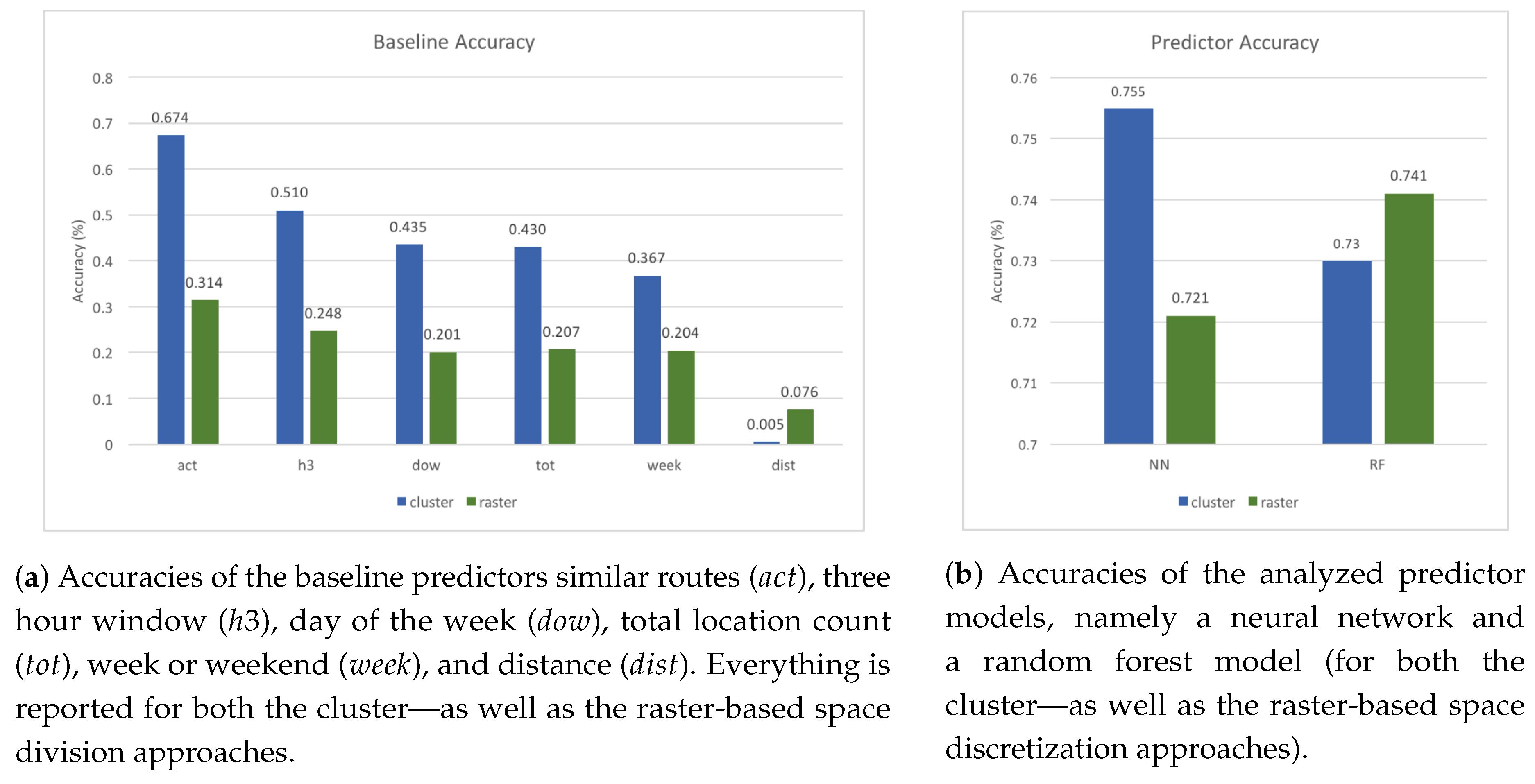
Figure 2a reports on the prediction accuracies that can be achieved by the baseline models alone. Each of these accuracy values describes the ratio between the number of correctly predicted and the total number of samples. It can be seen that the similar routes ($act$) baseline prediction performs best, which can be explained by its elaborate comparisons to previous movements. As the movements of many people show high regularity [44], if they travel a similar route, chances are high that the destination is also similar. Temporal patterns ($h3$, $dow$, $week$) also exhibit a good prediction potential, as does the total number of times a location was visited ($tot$). The former can be explained by the (usually) very regular temporal structure of movement and mobility habits, while the latter stems from the fact that the most visited place is usually home, where a user often will spend a significant amount of time. As such, all trackpoints leading up to the home location are typically predicted correctly, which represents a large share of correct predictions. Finally, the distance baseline performs very badly, as the nearest location is only infrequently the one someone is currently traveling to. Especially in the cluster-based approach, due to the trackpoints often being further apart than the average cluster size, numerous other clusters are closer than the actual next place.

4.3. Predictor Accuracy

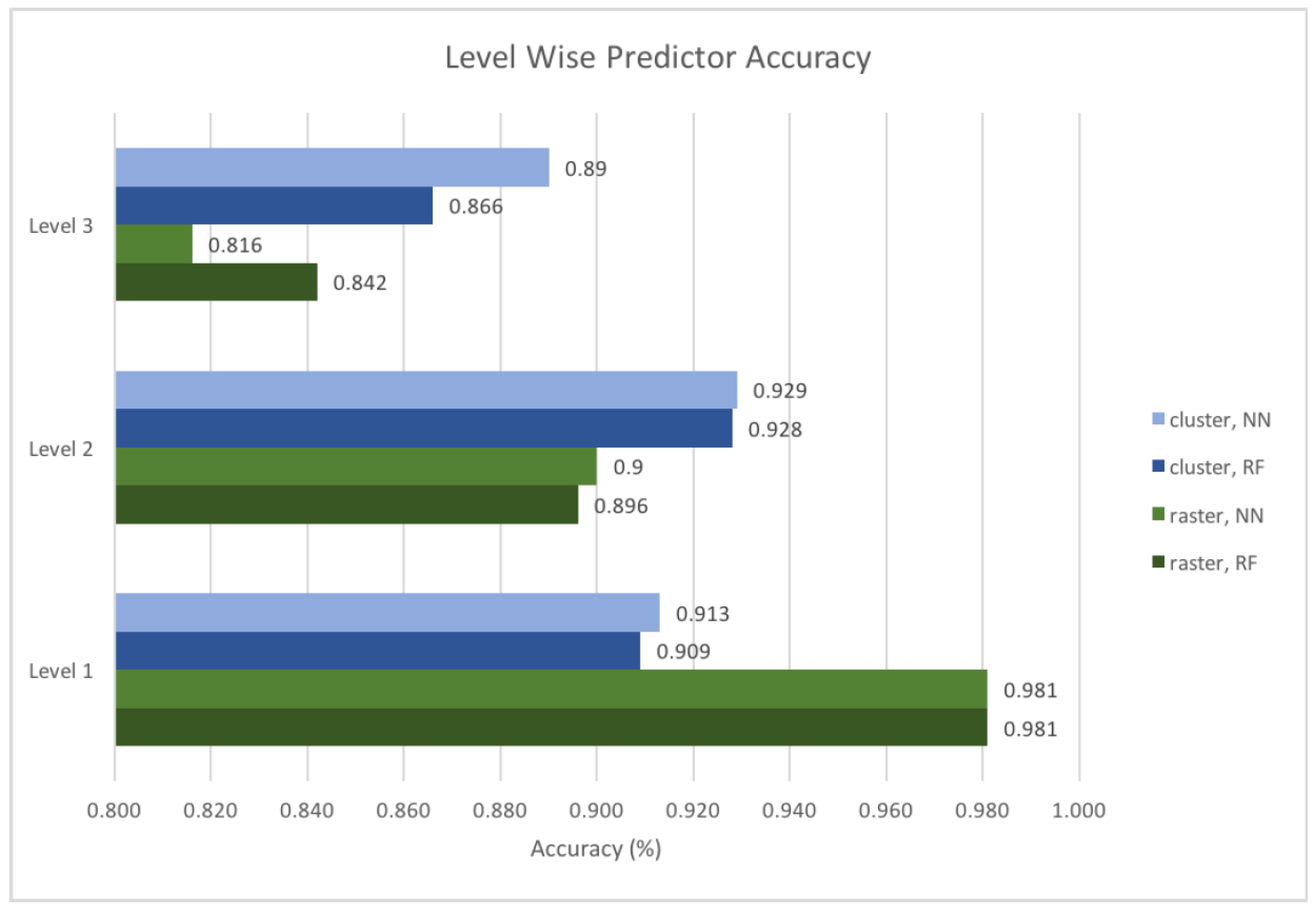
The predictor accuracy describes the ratio between the number of correctly predicted and the total number of samples in the case of the chosen machine learning approaches. As shown in Figure 2b, the predictors perform reasonably well, and achieve around 10% higher accuracy than the best baseline model. The best predictor accuracy of 75.5% is achieved when using a NN in combination with a clustered location input, followed by the performance of a random forest model with rastered input. The predictor accuracy can be broken down to each level of the hierarchy as demonstrated in Figure 3. Since the prediction system is hierarchical, the next place needs to be predicted correctly at every level to achieve a correct overall prediction (however, note that in Figure 3 we consider the prediction accuracy on each level individually). It can be observed that the NN and random forest models produce similar results when being provided with the same input. In general, the neural network performs similar or slightly better than the random forest in most cases, except for level three with the rastered input.

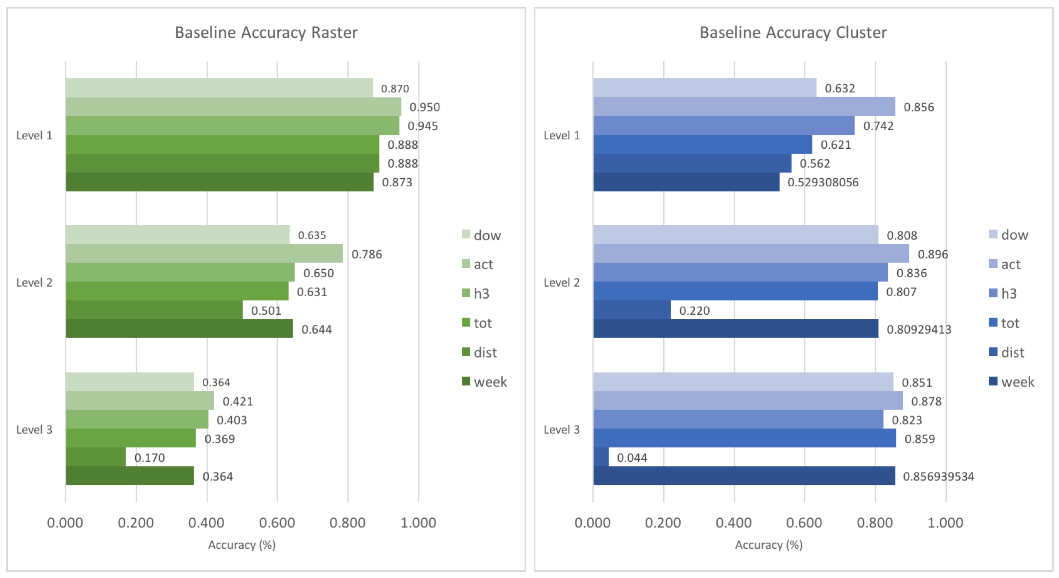
Figure 4 shows the same accuracies of the baseline features. It can be seen that especially the predictive power of the spatial context (denoted primarily by the distance feature dist) decreases faster with increasing spatial resolution than the others. This means that at higher spatial resolutions, the distance to a potential next place plays a minor role, most likely because these next places are closer to each other and do not differ much in terms of distance. On the other hand, temporal context such as the weekend indicator (week) show relatively more predictive power at higher spatial resolutions which can be explained as these features have a more discriminative value (e.g., on the weekends people will usually visit very different places than during the week). In the case of the raster-based approach, the prediction accuracy decreases for all features with increasing spatial resolution. This is in contrast to the cluster-based approach, where individual features reach higher prediction accuracies at higher spatial resolutions. The reason for this is to a large degree that in a raster-based approach space is divided at arbitrary boundaries, thus leading to a lot of wrong predictions.

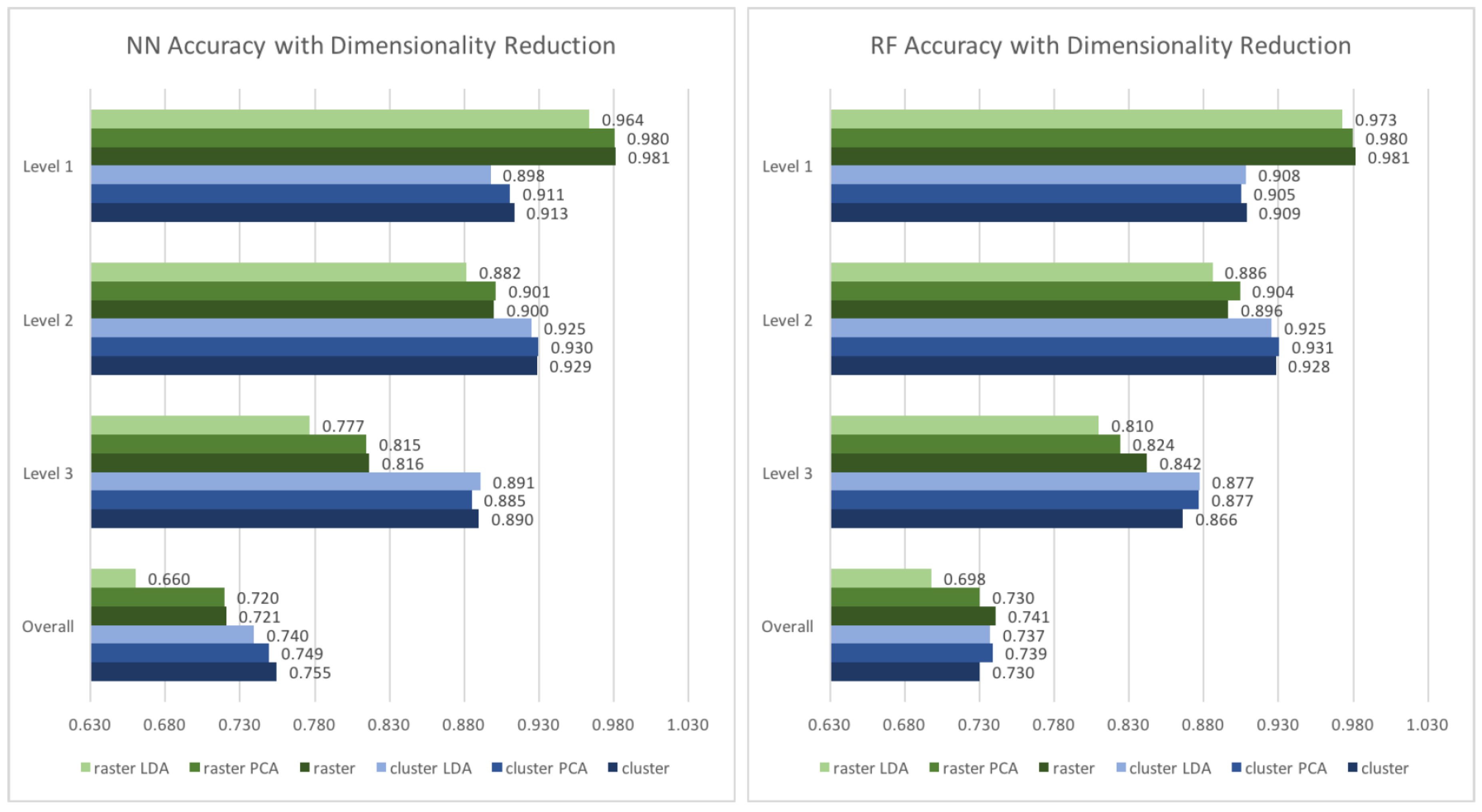
To reduce the number of dimensions, linear discriminant analysis (LDA) and principal component analysis (PCA), two different dimensionality reduction algorithms, were tested. As indicated in Figure 5, the dimensionality reduction method does not improve the prediction performance in most of our cases. Overall, the neural network performs better with the original input, while the results for the random forest model are slightly different: With the clustered input, it performs marginally better if LDA or PCA is applied. Nevertheless, the differences are of a degree (0.7–0.9%) which does not justify a general application of a dimensionality reduction method for the features used within this work.

Since there are some variations within levels of scale, the best configuration is chosen for each individual level.

Table 3. Next place prediction accuracies when using the best prediction model on each level. Even though there are some improvements of the prediction accuracy, the overall improvement is small, at the cost of a more complex prediction method involving different types of machine learning models.

	Level 1	Level 2	Level 3	Overall Accuracy	Improvement
Cluster	NN, original	RF, PCA	NN, LDA	75.7%	0.26%
Raster	RF, original	RF, PCA	RF, original	74.7%	0.64%

shows the best configuration for the clustered and the rastered inputs on each level of scale of prediction. For the clustered input, the prediction accuracy can be improved by 0.3%, while for the rastered input, the improvement can be up to 0.6%.

4.4. Deviation Measures

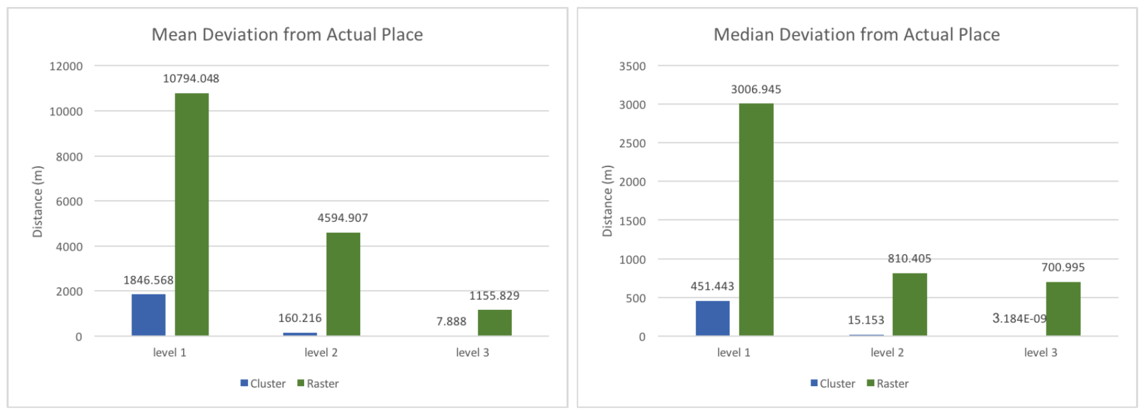
As explained in Section 3.1, we propose an optional step to predict exact coordinates rather than merely a cluster or cell id, as based on the level 3 prediction. For this purpose, we take the coordinates of the centroid of all locations visited by a single user within the predicted cluster as the prediction. The deviation of the distance between the predicted coordinates and the actual location (the ground truth) can be used as another indicator for rating the prediction quality. Figure 6 shows the mean and the median deviations of this distance. As expected, the deviations decrease with lower levels, because on the highest level the clusters resp. cells are of such size that even a correct location prediction can result in a substantial distance deviation. In general, both the mean as well as the median deviation is much smaller for the clustered input.

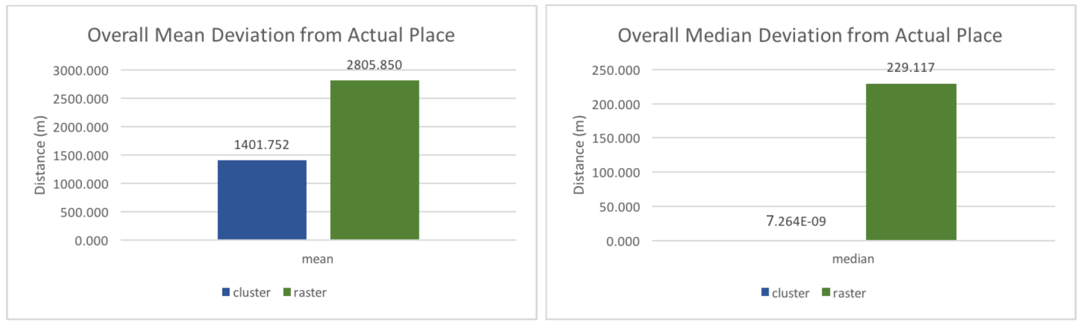
To calculate the overall distance deviation, the deviations from wrong predictions in level one, two, and three are collected, to which all the distance deviations from correct predictions in the third level are added. As shown in Figure 7, the mean and the median are much smaller for the clustered input, which indicates that the model’s performance is much better with this type of input. One can see that for 50% of the predictions, the distance deviation of the prediction is practically zero using the cluster model, and around 230 m using the raster-based approach. There are two reasons for this very exact prediction when using the clustered approach. First, many clusters contain exactly one location for a single user. As such, if the cluster id is predicted correctly, the resulting distance deviation is zero, as the user necessary needs to end up at exactly this location (note that while the sample is not used for training its location is represented in the clusters). Second, many level three clusters only contain one location, as they were constructed from level one or two clusters that contained less than 30 points. That means that each point forms its own cluster, and if the cluster is predicted correctly the resulting distance is zero. 22% and 78% of the clusters are represented as a single point in the second and the third level respectively, which means that chances are high that the distance deviation is zero, provided that the prediction is correct.

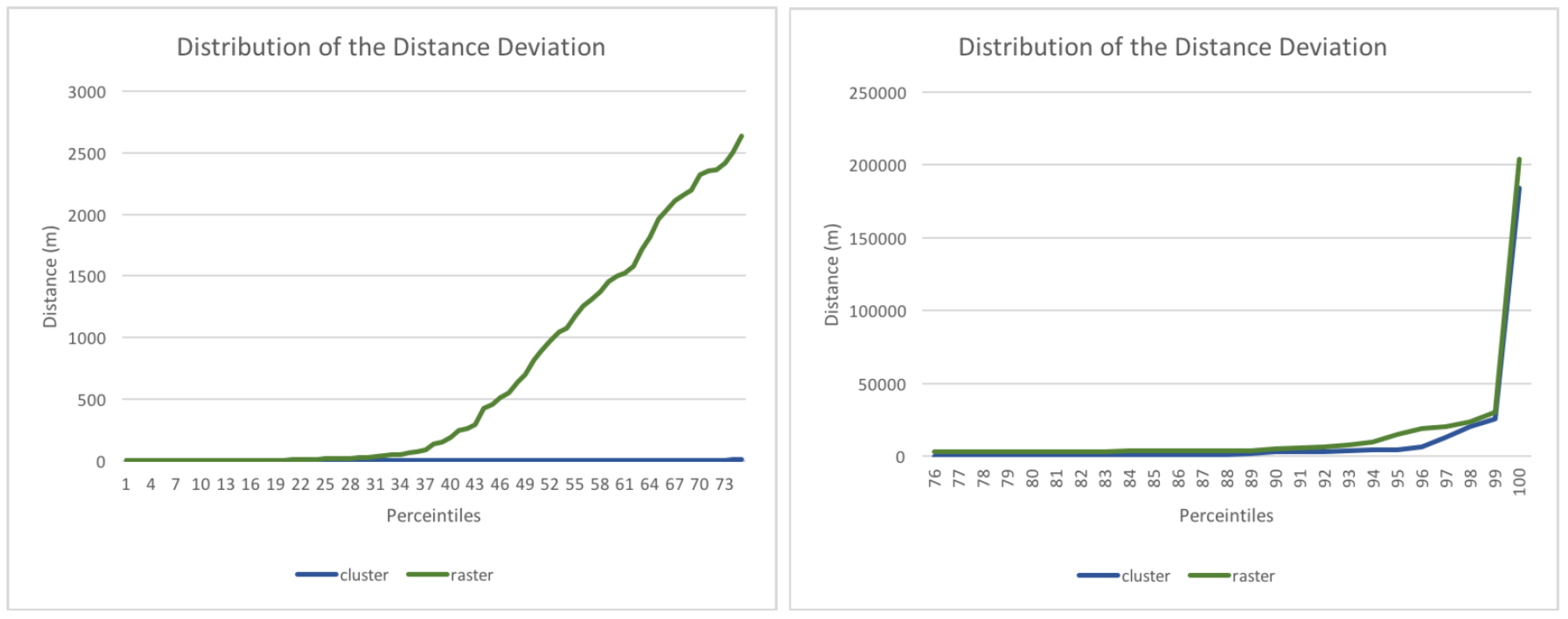
The large difference between the mean and median of the distance deviation can be explained by several outliers with huge distances. Figure 8 shows that in the first quartile the distributions of the clustered and rastered approaches are similar. Then, however, the distance deviation of the rastered input increases dramatically. The difference between the two inputs is significant in the last quartile as well, which proves that the clustered input is superior in terms of distance deviation. A drawback of the here proposed hierarchical approach is that if a cluster is wrongly predicted on the first level, it might lead to huge distance deviations. The last percent clearly shows this, as in this case level one clusters are predicted that are very far away from the actual location of the user.

4.5. User Accuracy

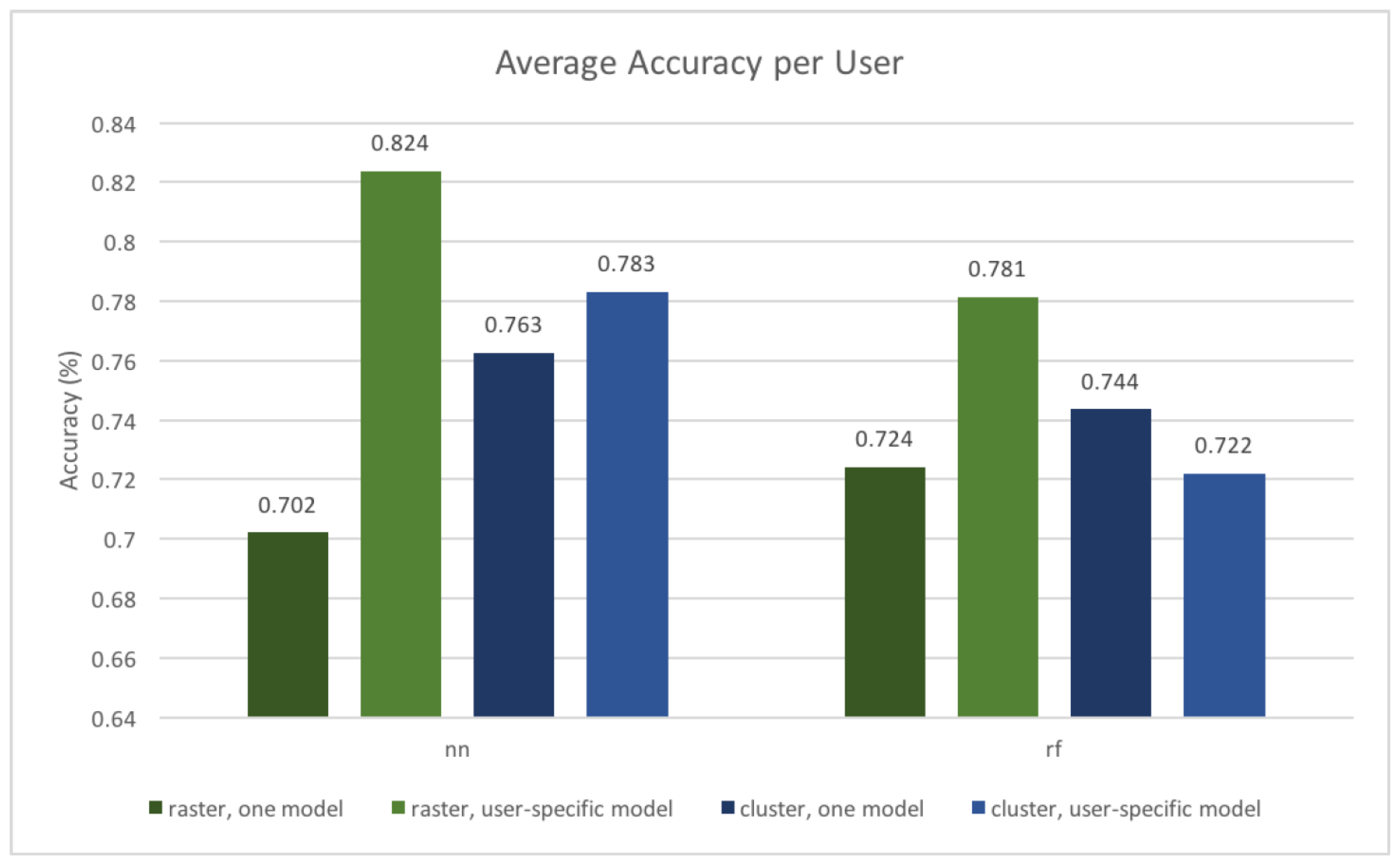
When analyzing the accuracy of predicting each user’s next places individually (but using a single model trained on data from all users), we found that only for three users the accuracy is less than 60% (using the neural network as a predictor of clustered locations). The weakest performance is for a user with a prediction accuracy of 15.3%, while the other two were in the range of 40–60%. We found that this user constantly visited numerous new places, which of course are difficult to correctly predict. To further elaborate on the user-specific accuracies, we trained the same models based on data from each single user alone (which is usually done for prediction models, but is an approach that suffers from the cold start problem). Figure 9 shows the resulting model accuracies.

As one can see, all models perform rather well with accuracies ranging between 70.2% and 82.4%. The neural network performs better with a user-specific model, which is not surprising since it is able to learn a user’s patterns better, without being influenced by other users. It is interesting to see that the user-independent model performs better in the case of a cluster-based approach with a random forest model (showing an improvement from 72.2% to 74.4%), while in all other cases the user-specific models show a higher accuracy. In general, the cluster-based methods show a smaller difference, which is likely due to the raster-based methods splitting at arbitrary boundaries, and thus leading to more wrong predictions when data from all users is used to train the model.

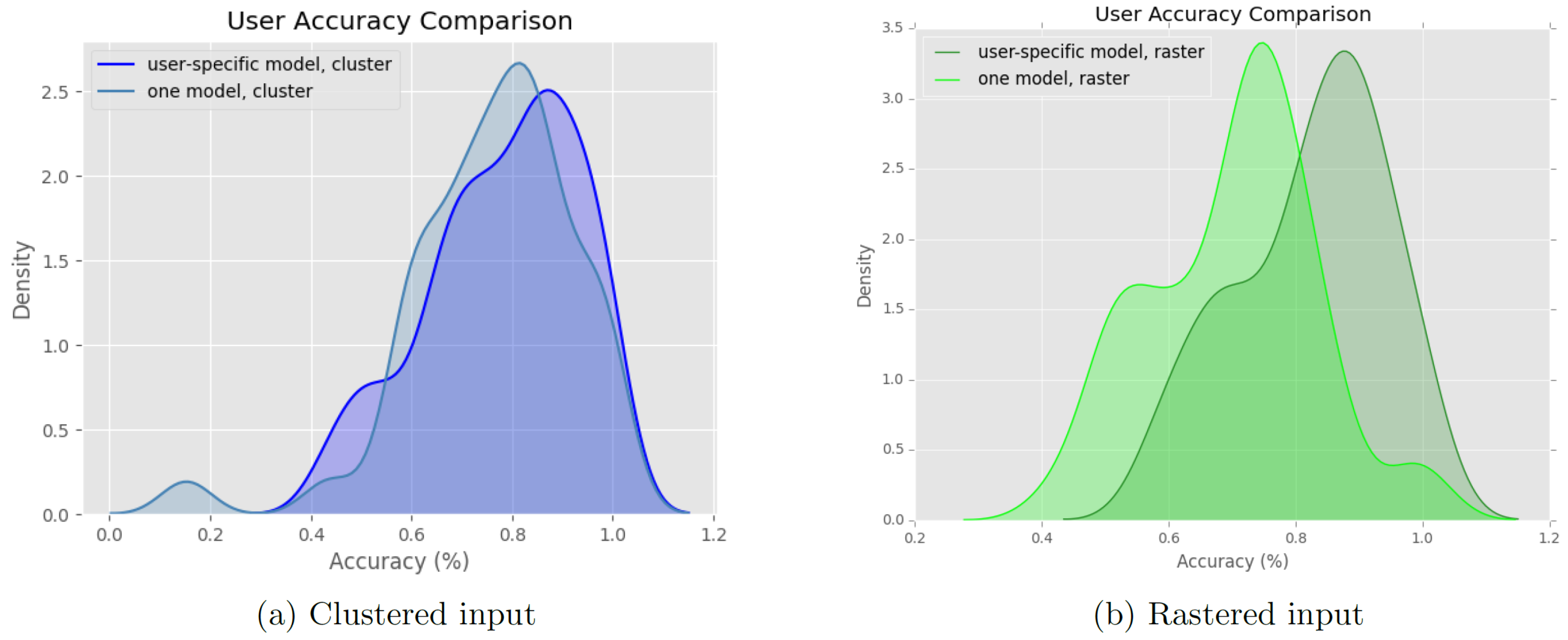
Figure 10 provides more insights into the differences between user-independent and user-specific models. The latter suffer from the cold start problem and are unable to predict previously non-visited locations (in most cases). We found that only for the rastered input there are clear differences between the user-independent and user-specific models (where the user-independent model has a lower prediction power than the user-specific ones). This is because the user-independent model is more likely to make wrong predictions if the locations are split at arbitrarily borders (i.e., split into arbitrary raster cells). The effect of these wrong predictions is minimized when only data from one user is used, as this user is more likely to stay at only a few (non-split) locations.

4.6. Feature Importance

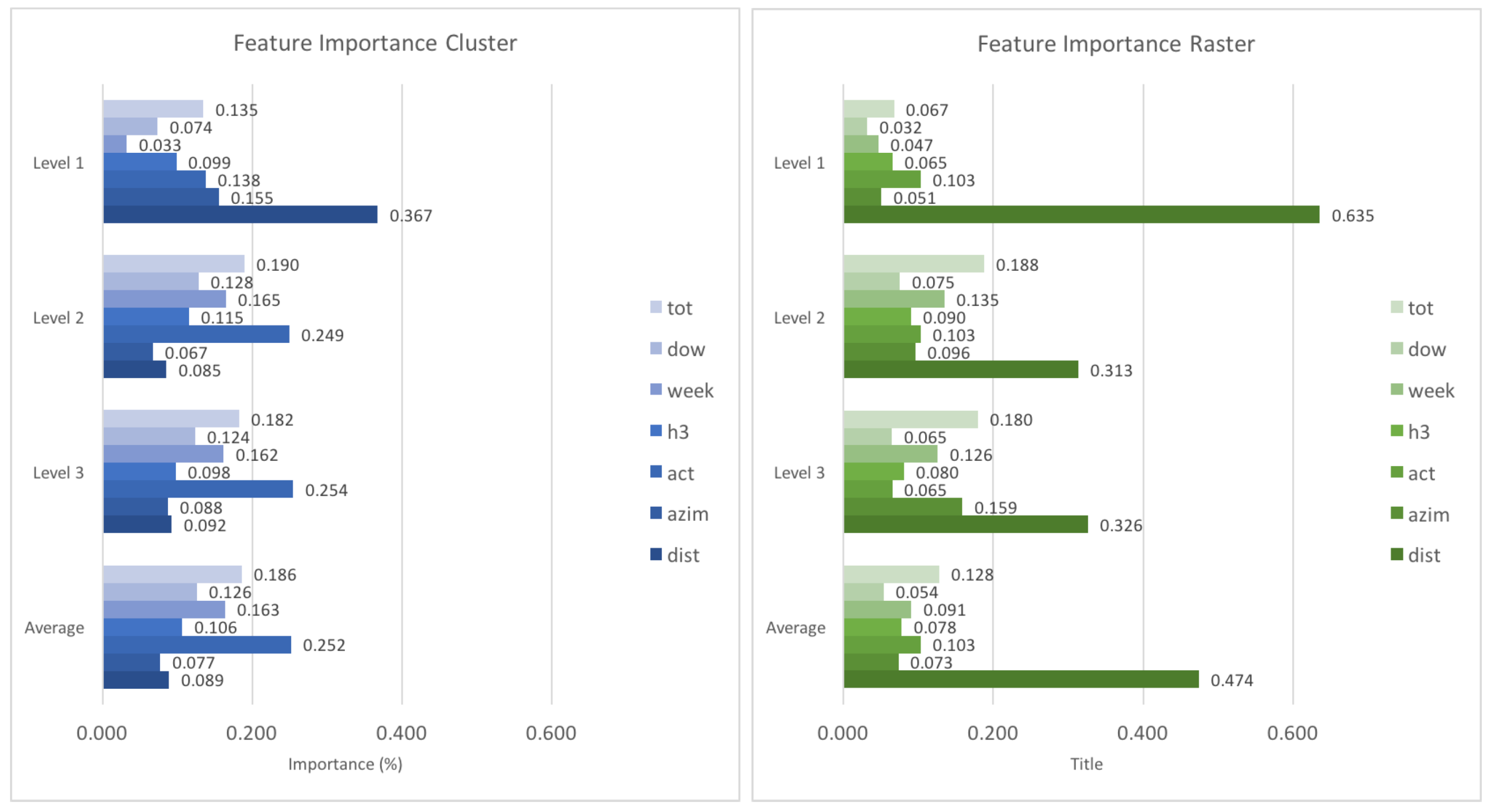
To assess the influence of different features on the prediction accuracy, we use the random forest to extract the relative feature importance on all levels of the prediction hierarchy. Figure 11 shows all resulting importance values. It can be seen that the distance is generally of high importance, in particular on level 1. The reason for this is that especially on higher levels of scale, people will either stay in the same cluster or cell, or travel to one which is relatively close. Interestingly, with an increase in spatial resolution, i.e., when going to lower levels of predictive scale, temporal characteristics of movement (location context) increase in importance. The increasing importance of the $week$ feature is especially interesting, which serves to distinguish between weekly and weekend patterns. The $act$ (similar routes) feature is generally important, which corresponds to the relatively strong performance of the respective baseline.

5. Discussion and Conclusions

In this paper, we analyzed the effects of various input features and modeling choices on the prediction accuracy in a next place prediction problem, given a historical dataset of a multitude of users. Our approach uses a hierarchical structure, where space is subdivided into either raster cells or location clusters. This space discretization is performed on three levels, each of which increases the fine-grainedness of the next place prediction. As the problem transforms into a label prediction problem, we can employ machine learning techniques such as NN or random forests, both of which are extensively tested in the course of this research. From the movement trajectories of the users, we generate a number of user- and location-centered spatio-temporal context features (to be used within the machine learning method), such as if a location was visited during a certain time, or if it is spatially close or is in the direction of current movement. The effects of these input features and modeling choices is compared to several baseline predictors, which use a simple forecast based on a single input feature.

We employ all model combinations on a real-world dataset collected via smartphone from approximately 700 users over the duration of six months. While the tracking accuracy is not always very high, staypoints (i.e., locations where someone stays for a certain amount of time) are recognized reliably. As our approach is largely based on the prediction of staypoint clusters, it is not highly sensitive to the GPS sampling frequency. In a similar spirit, as the model uses data from all users at all locations, individual missing trackpoints due to GPS signal loss are not critical while training the model. During the prediction phase, a higher number of trackpoints leads to a marginally better outcome, as they are used within the azimuth and similar routes features. However, these two features themselves are not highly sensitive to the number of trackpoints, as long as more than two are available. The prediction accuracy of the approaches presented here is generally in the order of 75%, across all spatial layers (e.g., for the first and most crude spatial division the prediction accuracy is usually higher, as many people simply stay in the same cell or cluster in which they were before). The baselines are lower than that, ranging from almost zero to 67.4% prediction accuracy. Finally, we propose and evaluate dimensionality reduction techniques and exact longitude/latitude prediction, as well as models for each user individually.

Using only one prediction model for all users has several advantages: there is more data to train the model, predictions can already be made for new users (without data), and predictions can generalize in the sense that previously non-visited locations can be predicted for any user. The analysis presented in Section 4.5 showed a negligible prediction accuracy loss when using a user-independent model in favor over a user-specific model. However, having only one prediction model for all users leads to a large number of possible locations, which either requires a huge model, or some hierarchical approach like the one presented here. In contrast to one-level systems (e.g., [19,41,45]), which either only predict a small number of locations or are restricted to a smaller area, our approach is able to predict one of a million cells resp. 29,270 clusters for any user (where an average user only visited 18 cells or 41 clusters on level three). We found that the hierarchical model worked well, and allowed the users to have varying numbers of visited locations, which were automatically incorporated at the various levels. However, the here presented hierarchical structure has still room for improvement. While the spatial resolution and the number of subdivision cells were chosen with typical mobility behavior in mind, this also means that an average user only visits 1.7 raster cells (out of 100) resp. 3.4 clusters (out of 30) on the first level, numbers which do not change greatly on the following levels. A potential improvement would be to adapt the number of cells and clusters on each level to the ones actually visited. This would make the prediction easier, while reducing the expressiveness of the model. However, since the prediction is refined on the following levels, this reduction could be acceptable.

Generally, both the neural network as well as the random forest demonstrate an acceptable performance. Our analysis yield that the random forest model performed marginally better with the rastered input, while the NN achieved a higher prediction accuracy on the clustered input. A similar take-away can be formulated for the baselines: They yield a higher prediction accuracy for the clustered input than for the rastered input. A prominent reason for this is that rasters divide space in a way that is not related to the input data, meaning that many locations that should logically be grouped are split. This makes it more difficult for the baselines, which always predict the most extreme location—if many locations are on the edge of this cell, a much larger share will be wrongly predicted than in the cluster-based approach. One can also see that while the random forest tends to perform better at higher spatial resolutions (level three), i.e., in general the NN working on larger (clustered) feature space incorporating both spatial and temporal features should be preferred at lower spatial resolutions, while on the scale of several 100 m a raster-based approach with random forests is a viable alternative.

In terms of exact coordinate predictions, the clustered approach performs much better. One has to consider that on average, clusters are much smaller in size compared to raster cells on the same level of scale, but even after normalizing the distance deviations (where the normalization factor was determined from the average distance of randomly predicted locations to the actual location) the longitude/latitude predictions derived from cluster locations are much more accurate than raster predictions. However, the rastered input still has the advantage that the clustering does not have to be performed for newly added location data and thus the model can simply be refined without changing its entire shape.

Interestingly, the seven different context features analyzed within this work performed very differently depending on the input type (rastered vs. clustered). On the first level, the distance feature is used prominently for the prediction. This makes sense, as most of the times people stay in the same raster cell or cluster, which is easily identified by the distance feature. On the lower levels, the distance becomes less important, as people frequently change to locations at farther distances. Generally, the temporal (location based) features are less important when working with the rastered input, as the arbitrary division of space splits up logically connected locations into different cells. The similar routes ($act$) feature shows a high prediction accuracy when used as a baseline, but is also very important for the NN and random forest models. This is interesting, as this is the only feature that incorporates information from past routes, which hints at the importance of not only using trackpoint histories (as in the azimuth feature), but take into account all previous routes. It could be an interesting future extension to increase the number of features which take previous routes into account, possibly combining these with temporal characteristics such as on which day of the week a certain route was traveled.

Table 4. Ranking of all features across the different levels and input methods.

	Clustered Input			Rastered Input
	Level 1	Level 2	Level 3	Level 1	Level 2	Level 3
1.	$dist$	$act$	$act$	$dist$	$dist$	$dist$
2.	$azim$	$tot$	$tot$	$act$	$tot$	$tot$
3.	$act$	$week$	$week$	$tot$	$week$	$azim$
4.	$tot$	$dow$	$dow$	$h3$	$act$	$week$

shows the importance of various features on different levels, both for the clustered as well as the rastered input. It can be seen that the spatial (user based) features play a big role mostly on higher levels, while temporal (location based) features such as $week$ or $dow$ become more important on lower levels. A second observation is that the distance keeps its importance for the rastered input, while it does not play a big role in the clustering case after level 1. However, the feature importance as given by the random forest resp. decision trees should be taken with caution, as it can show a bias towards variables with many categories and continuous variables (such as $dist$).

6. Outlook

An analysis as presented in this paper cannot cover all possible modeling choices and parameters. Particularly interesting avenues for future research are along the lines of determining the relationship between spatial resolution (as for example encoded in our hierarchical approach) and the importance of various temporal, spatial, or other features. This becomes increasingly relevant as mobility and movement prediction becomes more and more important with automated and autonomous transport systems, such as self-driving cars. A hierarchical approach could also use different prediction models and methods depending on the spatial resolution and the task at hand (cf. [9]), and incorporate an automated approach for determining the optimal number of levels and their spatial scales. Furthermore, our work could be extended by testing additional classification algorithms and methods.

In a similar spirit we found that more complex features, such as the similar routes one can provide a good basis for prediction. Not only would searching for such informative features make sense, but their structure could be embedded in the machine learning model directly. For example, recurrent neural networks use historical outputs as inputs for next predictions, making them well suited for continuous prediction tasks like the one discussed here. On the other hand, convolutional neural networks are successfully applied in computer vision tasks, which are inherently spatial as well. Adapting such networks to the problem of mobility and movement prediction could make elaborate feature engineering obsolete by letting the model find and learn relations without any help from a domain expert.

We compared several baselines against some of the most commonly used machine learning models, as we were interested in assessing the influence of various contextual factors at different spatial resolutions. However, it is left open how these models compare to other well-known models, such as support vector machines, hidden Markov models or conditional random fields. For a future continuation of this line of research, we envision a more thorough treatment of next place prediction, not only including various features and model parameters, but also a larger number of different machine learning approaches. This will further help giving researchers a more solid understanding for building next place prediction models.

As next place prediction is a potentially continuous task (e.g., in the case of autonomous mobility), it is important to design models in a way that they can constantly learn from incoming data streams. The here presented clustering approach is less suited to this, as clusters may have to be recomputed in case a new staypoint lies outside any of the known clusters. While the raster-based approach does not suffer from this issue, it has other drawbacks. A method that combines both approaches, while at the same time not suffering from a cold-start problem (in which prediction of new users without data is impossible) and being able to use data of all users in the system would be highly desirable.

Finally, the proposed method was evaluated and analyzed on a dataset consisting of 41 users tracked over approximately six months. While splitting the data into training, test and validation sets allowed us to study various modeling choices solely using this data, it would be interesting to see how the approach performs with different data, e.g., solely from mobile phone tracking using cell towers or more accurate GPS traces.