Article

An Open-Boundary Locally Weighted Dynamic Time Warping Method for Cropland Mapping

1
State Key Laboratory of Resources and Environmental Information System, Institute of Geographic Sciences and Natural Resources Research, Chinese Academy of Sciences, Beijing 100101, China
2
University of Chinese Academy of Sciences, Beijing 100049, China
3
Department of Geography and Anthropology, Louisiana State University, Baton Rouge, LA 70803, USA
*
Author to whom correspondence should be addressed.
ISPRS Int. J. Geo-Inf. 2018, 7(2), 75; https://doi.org/10.3390/ijgi7020075
Submission received: 28 December 2017 / Revised: 15 February 2018 / Accepted: 18 February 2018 / Published: 23 February 2018

Abstract

:
This paper proposes an open-boundary locally weighted dynamic time warping (OLWDTW) method using MODIS Normalized Difference Vegetation Index (NDVI) time-series data for cropland recognition. The method solves the problem of flexible planting times for crops in Southeast Asia, which has sufficient thermal and water conditions. For NDVI time series starting at the beginning of the year and terminating at the end of the year, the method can separate the non-growing season cycle and growing season cycle for crops. The non-growing season cycle may provide some useful information for crop recognition, such as soil conditions. However, the shape of the growing season’s NDVI time series for crops is the key to separating cropland from other land cover types because the shape contains all of the crop growth information. The principle of the OLWDTW method is to enhance the effects of the growing season cycle on the NDVI time series by adding a local weight to the growing season when comparing the similarity of time series based on the open-boundary dynamic time warping (DTW) method. Experiments with two satellite datasets located near the Khorat Plateau in the Lower Mekong Basin validate that OLWDTW effectively improves the precision of cropland recognition compared to a non-weighted open-boundary DTW method in terms of overall accuracy. The method’s classification accuracy on cropland exceeds the non-weighted open-boundary DTW by 5–7%. In future studies, an open-boundary self-adaption locally weighted DTW and a more effective combination rule for different crop types should be explored for the method’s best performance and highest extraction accuracy for cropland.

1. Introduction

Global agricultural production will likely need to increase in the future due to population growth, changing diets, and the rising importance of bioenergy [1]. Cropland mapping is an important part of land-use/land cover (LULC) mapping. Mapping cropland distribution [2,3] and monitoring crop growth status [4] as well as forecasting crop yield [5,6] using remote sensing data have been popular remote sensing applications. Timely and effective observation of the distribution of cropland in Southeast Asia is important for the food security of people living in the region. There have been recent studies focused on land cover mapping or crop mapping in Southeast Asia [3,7]. To obtain seasonal information on crops and separate rice paddy fields from dryland fields, time-series remote sensing data are usually used to extract cropland distribution information [8,9,10].
Time-series datasets for the Normalized Difference Vegetation Index (NDVI) or Enhanced Vegetation Index (EVI) have been used widely for cropland classification [11,12,13]. The datasets are provided by high revisit cycle frequency satellites such as NOAA/AVHRR, SPOT/VEGETATION, and Terra or Aqua/MODIS. Methods for time-series remote sensing data classification and their drawbacks and advantages for cropland extraction include:
  • Classifying ordered and stacked time-series data by SVM, random forest or other statistics-based supervised classification methods [14]. In these methods, the highly structured time-series information is usually ignored because this method does not treat Vegetation Index (VI) time-series data as a three-dimensional array in space.
  • Clustering method [15]. This method is generally used for classifying cropland for land-cover products. Some global land cover mapping products such as GlobCover use the clustering of multi-spectral remote sensing time-series data. However, this clustering method cannot identify the seasonal information of crops.
  • Phenology-based method [16]. Different crops have different growing phenology. This method first extracts phenology traits from time-series data such as the start and end of the growth season, then matches the phenology traits with specific crop types. Some phenology traits, such as growing season amplitude, length, and curve slope, are not necessarily calculated based on fixed cultivation times, so the method is also suitable for cropland extraction in Southeast Asia [17]. The essence of the phenology-based method is tracing critical points on VI curves.
  • Multi-phase analysis method. A method proposed by Xiao et al. [9] is a representative method using multi-phase analysis for rice paddy field extraction. This method traces the particular feature points on a VI time series counterpart with the corresponding category of crops for crop extraction. For example, the transplanting stage of a rice paddy could cause impounded surface water, which is a characteristic distinct to rice plantations. However, this method is only useful for crops with particular growth stages such as rice paddy fields.
  • Classifying with auxiliary data [18]. Some methods also used the remote sensing time-series data combined with auxiliary data such as meteorological data to classify cropland. This kind of method is similar to a decision tree, first using auxiliary data to divide a region then classifying it using remote sensing images inside the region.
  • Other picked updated methods [19,20,21]. Some methods using the Google Earth Engine for automated cropland mapping at large-scale [19]. Some methods using the data fusion technique for extraction of cropland [20,21].
  • Mining the time-series information. Different surface features have different remote sensing time series shapes. There are plenty of methods mining the shape of time series characteristics to classify land-cover as well as croplands, for example, time-series information mining based on statistical methods [22] or neural networks [23]. As a potential mining tool for time-series information and for extracting information provided by remote sensing time-series data, time series similarity measures have also been used for cropland classification or land-cover classification in recent years.
Various approaches to measuring similarity exist in the literature and many of them are used for remote sensing classification. Geerken et al. applied the Fourier filtered cycle similarity method to identify rangeland vegetation types [24]. DTW (Dynamic Time Warping) distance is a shape-based time series similarity measure method. The algorithm compares two time series and finds their optimal alignment, providing a dissimilarity measure as a result [25]. DTW is very good in dealing with temporal drift [26]. Petitjean et al. applied the DTW distance to K-means clustering for land-cover classification and developed an average method to fit a multi-spectral remote sensing time series to K-means clustering [27,28,29]. Our previous study applied the DTW distance to identify rice paddy fields [30]. Maus et al. improved the DTW method for land-use and land-cover mapping by adding a time-weighting to constrain warping distance between two time series and extended the single split year into multiple years. All of these efforts have tried to mine remote sensing time-series information and improve the classification accuracies of specific problems. However, all of these approaches have not considered counterpoises to some applications in remote sensing, such as some sections of the time series being more important than other sections for time series similarity measures. For example, when identifying crops, the similarities between the growing season cycles are more important than the similarities between non-growing season cycles.
In this paper, we propose an open-boundary locally weighted dynamic time warping (OLWDTW) method for cropland mapping, where rice cultivation and field crops are separated in the extraction process. OLWDTW is based on open-boundary dynamic time warping. We selected open-boundary dynamic time warping because it is suited for the flexible planting season condition of crops of Southeast Asia [30]. Without time constraints when comparing time series similarities, open-boundary dynamic time warping is able to align any phase excursion between two NDVI time series. For example, the growth cycle of rice lasts for about four months, and the growing season of the reference NDVI time series might be from July to November while the test pixel for the rice plantation might show growth from February to June. These two NDVI time series of rice are excessively warped in the offsets of the growing season section. Still, the open-boundary dynamic time warping method is able to align the section of the growing season curve as shown in Figure 1. However, excessive alignment of curves also causes problems, such as when the warping is too extreme, or the warping cost distance of the whole NDVI time series of the final distance surpasses the distance of the growing season section such that identification of crops is difficult [31]. In our study, by adding a weight on the section of the seasonal growing curve, we can weaken the effect of the less important comparison of similarities between non-growing season cycle sections on the NDVI time series as well as reduce the effects of excessive alignment. Similarity measures between the two curves mainly focus on the growing season section, thus improving the identification accuracy.
The rest of the paper is organized as follows. In Section 2, we introduced the materials we used for the experiments. The proposed OLWDTW is described in detail in Section 2. Section 3 shows the experiment results, accuracy validations, and comparisons with an ordinary DTW method on two satellite datasets. The advantages and some future work are also discussed in Section 3. The conclusion is provided in Section 4.

2. Materials and Methods

2.1. Study Area

Two sites were selected to test our method. Both are near the Khorat Plateau in the Lower Mekong Basin (LMB), as shown in Figure 2. The location of the first site is 16°37′ N and 102°28′ E. The first site extends about 1914.1 km2 and includes a total of 175 × 175 MODIS pixels. The location of the second test site is 15°17′ N and 102°59′ E, extending 5606.3 km2 and contains a total of 276 × 325 MODIS pixels. The reason for selecting these areas for testing our method is because we had the validation classification maps of these two sites, provided by the Land Development Department at the Office of Soil Resources Survey and Research, for manual interpretation.
Within the LMB, the Mekong Delta in Vietnam and the Khorat Plateau in Thailand are the two most important regions, together accounting for nearly 80% of the total LMB rice paddy production. The Khorat Plateau is located in the northeastern part of Thailand. On the Khorat Plateau, the soil is mostly sandy, making water retention almost impossible and resulting in generally dry conditions unfavorable for widespread cultivation. However, the Mekong River flows past much of the northern and eastern edge of the region, enabling local cultivation in several provinces. This region, with a total planted area of 5.5 million ha, generally grows one important crop each year, mostly grained rice, with a very small second crop. Given the undulating terrain, irrigation is limited, and the average size of rice farms is smaller than in other regions. Most of Thailand’s jasmine rice, or Hom Mali, is produced in this region [32].
According to the validation classification map provided by the Land Development Department at the Office of Soil Resources Survey and Research, the mean plot size of the rice paddies is 0.5 km2 in test site 1 and 1.46 km2 in test site 2. The mean plot size of the dryland crop in test site 1 is 0.14 km2 and 0.15 km2 in test site 2.

2.2. Satellite Data and Preprocessing

The study mainly used MODIS time-series data for classification. The MODIS data product was retrieved from the online Data Pool, courtesy of the NASA Land Processes Distributed Active Archive Center (LP DAAC), United States Geological Survey (USGS)/Earth Resources Observation and Science (EROS) Center; specifically, the MOD09Q1 data for 2015 were used. MOD09Q1 provides MODIS bands 1–2 surface reflectance at 250-m resolution. Landsat 8 OLI data were obtained for geometric correction. Landsat 8 OLI data were obtained from the USGS website (https://earthexplorer.usgs.gov/). We obtained high-quality imagery (cloud cover less than 10%) in the Path 128 Row 49 scene for 18 March 2015.
We obtained the two bands of the MOD09Q1 data using the MRT tool for NDVI calculated with Equation (1). Tiles h27v07 covered the two test sites of this study [33].
NDVI = ( ρ nir ρ red ) ( ρ nir + ρ red )
where ρ nir is the reflectance value of the NIR band of the MOD09Q1 data and Landsat 8 data and ρ red is the reflectance value of the red band of the MOD09Q1 data and Landsat 8 data.
To reduce the noise for better use of the NDVI time-series data, we used the adaptive S-G (Savitzky–Golay) filter in the TIMESAT software (version 3.1) [34] to reduce noise in the MODIS NDVI time-series data. The parameters in TIMESAT were set as follows: a window size of 4 for the filter, adaption strength of 2, and the number of envelope iterations was set to 3.

2.3. Open-Boundary Locally Weighted Dynamic Time Warping

2.3.1. Crop Identification Based on NDVI Time Series Similarity

Time-series data of continuous Earth observation-based estimates of vegetation have significantly improved our understanding of intra- and inter-annual variations in vegetation from a regional to global scale [35]. Application of remote sensing time-series data to classification based on NDVI time series similarity can be separated into two types. One is using the time series similarity measure for clustering, as in most of the work done by Petitjean. This method is more suitable to land-use and land-cover mapping [36]. Another approach is to first select a reference VI time series on the remote sensing images then use the time series similarity measure to obtain the similarity between the reference VI time series and the VI time series of every pixel. The more similarity there is between the reference and the pixel, the more likely it is that the pixel’s land cover type will be the same as the reference VI time series’ land cover type [31]. In this study, we used the second method to test our proposed algorithm because we only focused on the classification of croplands.

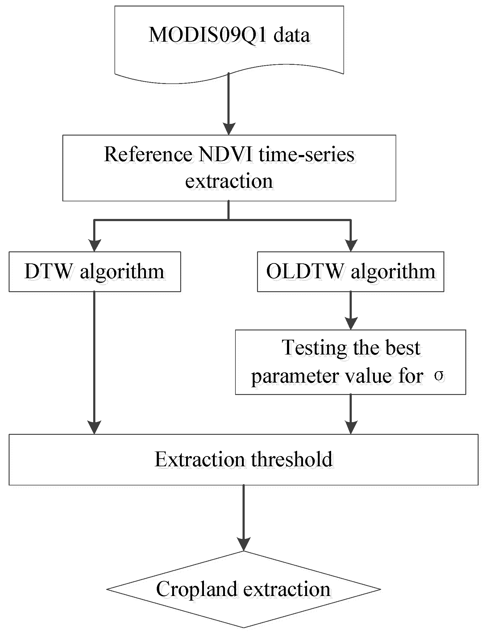
2.3.2. Review of Original Dynamic Time Warping

DTW uses a dynamic programming technique to find the minimal distance between two time series, where sequences are warped by stretching or shrinking the time dimension [37]. The DTW algorithm is described below.
Suppose that we have two time series, i.e., C = {c1, c2, …, cm} and Q = {q1, q2, …, qn}, with respective lengths of m and n. We construct an m × n matrix Am×n and define the distance between each element as aij = d(Ci, Qj) = ( C i Q j ) 2 . In the matrix Am×n, a warping path is set by a group of adjacent matrix elements, and notes for ω = {ω1, ω2, ..., ωk} and the kth element in ω are defined as ωk = (aij)k; this path must satisfy the following conditions:
  • Monotonicity constraint: ωk = aij, ωk+1 = ai’j’, then i’ ≥ i and j’ ≥ j
  • Endpoint constraint: ω1 = a11, ωK = amn
  • Continuity constraint: ωk = aij, ωk+1 = ai’j’; then i’ ≤ i + 1 and j’ ≤ j + 1.
Thus, DTW(C, Q) = min ( i = 1 K ω i ) . The DTW algorithm can be summarized by applying ideal dynamic programming to find the best (i.e., least bending) cost path, as shown in Equation (2):
{ d ( 1 , 1 ) = a 11 , d ( i , j ) = a ij + min { d ( i 1 , j 1 ) , d ( i , j 1 ) , d ( i 1 , j ) }
where i = 2, 3, …, m and represents the row index of the matrix and j = 2, 3, …, n and represents the column index of the matrix. D(i, j) is the minimum cumulative value of the warping paths.
The greater the distance between two time series, the more dissimilar the two time series are. The lower the distance between the two time series, the more similar the two time series are.

2.3.3. Local Weighting Added to the Seasonal Cycle Section

● General frame of the OLWDTW method
In the original version of DTW distance, the warping path is not limited by windows [31]. We call the original DTW (ODTW) algorithm the open-boundary DTW method. Although many applications use the window-restricted DTW for the best warping path search, we used the open-boundary DTW in this study and did not restrict the warping path.
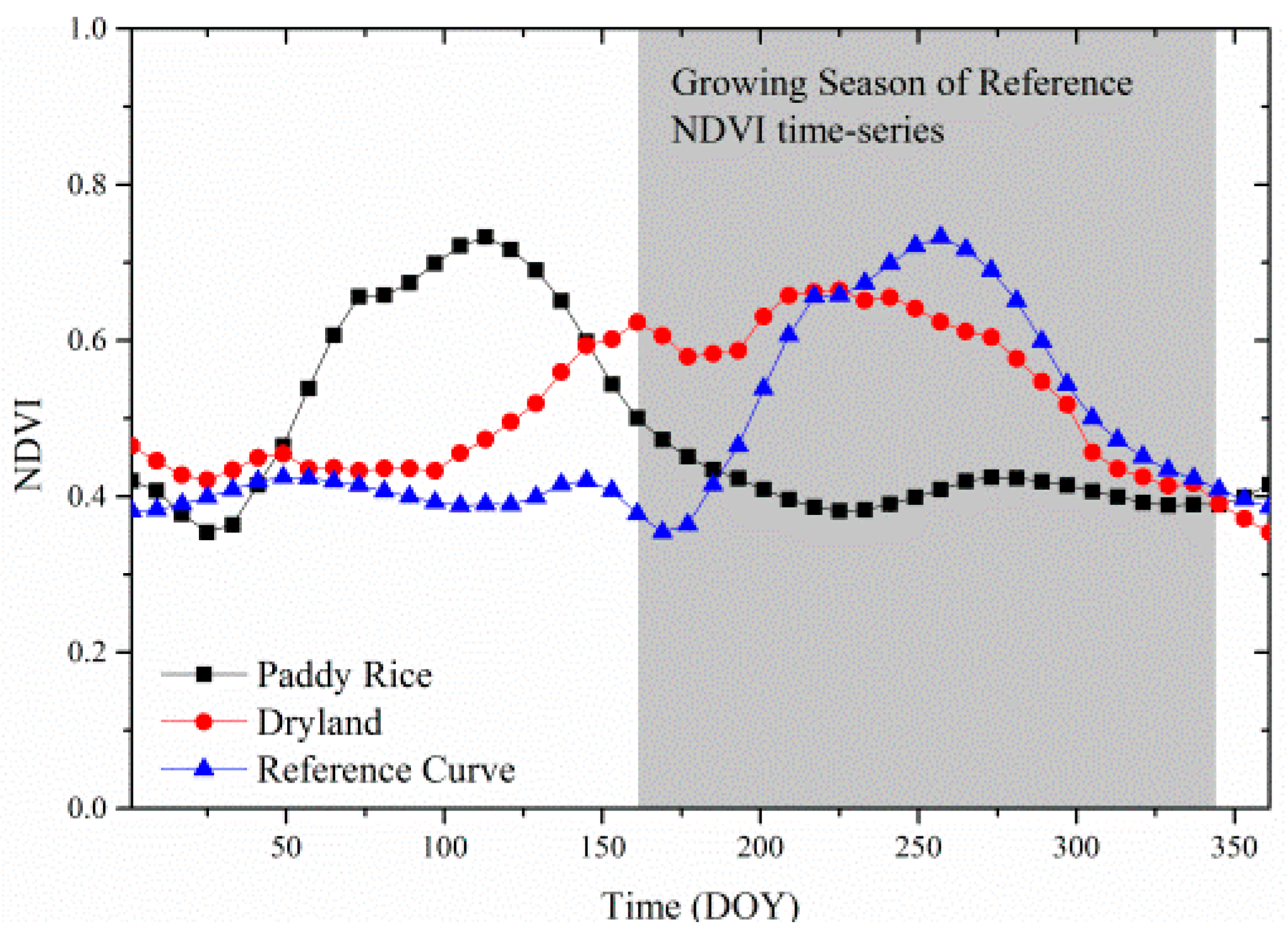
Sunlight, heat, and moisture conditions in Southeast Asia can affect when crops are planted. Identification of crops in remote sensing images of Southeast Asia should focus on the shape of the seasonal cycle rather than focusing on the beginning or the ending time of the seasonal cycle. For example, rice plantation could last from the 30th to 150th day of the year. It also could last from the 150th to 270th day. In either case, the seasonal growth cycle shape is similar. Enhancing the effect of the seasonal growth cycle when comparing the NDVI time series, while keeping the open-boundary characteristic of the original DTW algorithm, should help better recognize croplands. To enhance the effect of the seasonal cycle when comparing the NDVI cycle’s similarities, this locally weighted open-boundary DTW adds a coefficient σ to the section of the reference NDVI time series of crop types.
In Section 2.3.2, suppose time series C is the reference crop growth NDVI time series. C = {c1, c2, …, cm} and the growing season is from time i 1 to time i 2 , thus i 1 i i 2 . Add the coefficient σ to the section of the reference NDVI time series of crop types and Equation (3) becomes:
{ if   i 1 i i 2 then   D ( i , j ) = a ij + d ( i , j ) σ
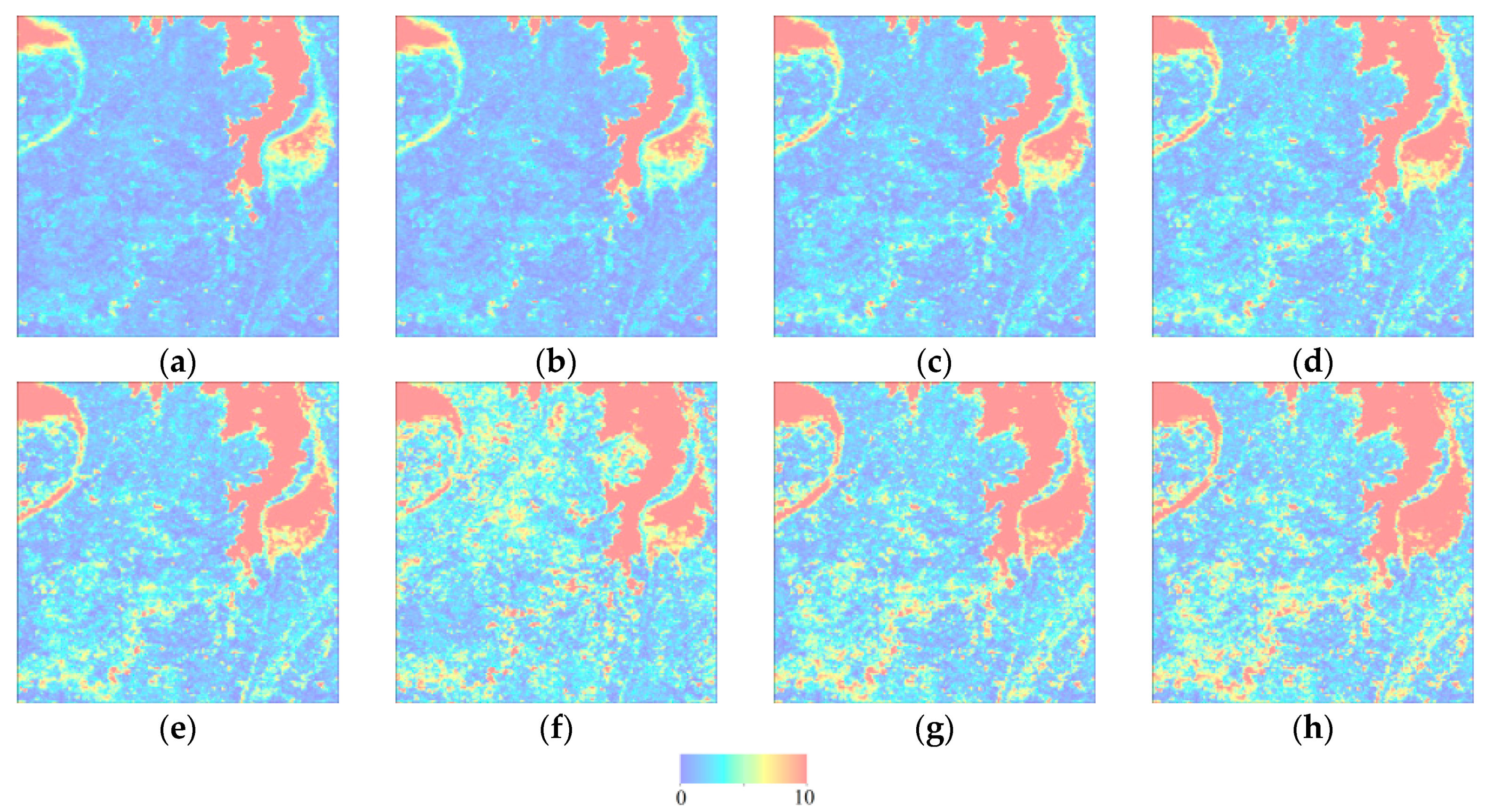
After running many tests using different values of σ, we found that for different crop types’ NDVI time series, the value of σ was different. The effectiveness of the OLWDTW method is illustrated by picking an NDVI time series from the satellite data and manually making a curve. As shown in Figure 3, the reference curve is the rice paddy cultivation field picked from the satellite data. The rice paddy curve is a man-made curve where the seasonal growth section on the curve from day 161 to day 345 is the same as the reference rice paddy curve picked from the satellite data. Using the original DTW algorithm comparing the distance between the reference rice paddy field curve with the manually made rice paddy curve and the dryland curve, the distance values are 0.5008 and 1.4333.
According to the reference rice paddy cultivation field, the growing season of a rice paddy field is from day 161 to day 345, so i 1 and i 2 
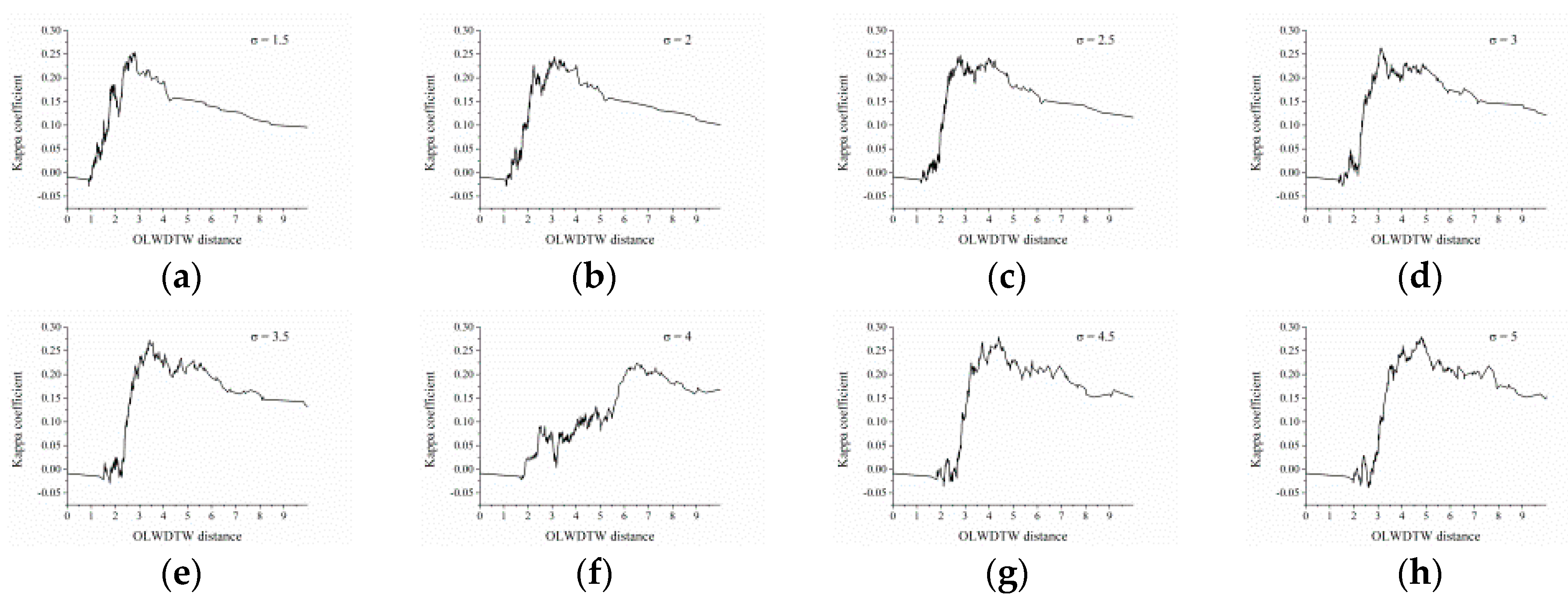
in Equation (3) are 20 and 43. Using the OLWDTW method to enhance the seasonal section on the curve according to Equation (3), we tested using different values of σ and the result is shown in Table 1. As the parameter σ grows, the value of OLWDTW distance are invariant between the reference curve with the rice paddy curve where the seasonal growth curve is the same as the reference curve. Not unexpectedly, the distance increases between the reference curve of the rice paddy field and the dryland crop field curve.
From the test above we can conclude that the open-boundary DTW is beneficial to cropland identification in flexible cropping conditions. The OLWDTW better distinguishes different crops. It seems to be that, as the value of σ increases, the rice paddy is increasingly better distinguished from dryland crops. However, in the real world, the seasonal growth cycles are not identical to the reference time series’ seasonal growth section cycle. In real-world testing we find that to make the best intra-class and inter-class distinction between crops and other land cover types, there exists an optimal σ value to distinguish cropland types.
● Parameter value selection for OLWDTW method
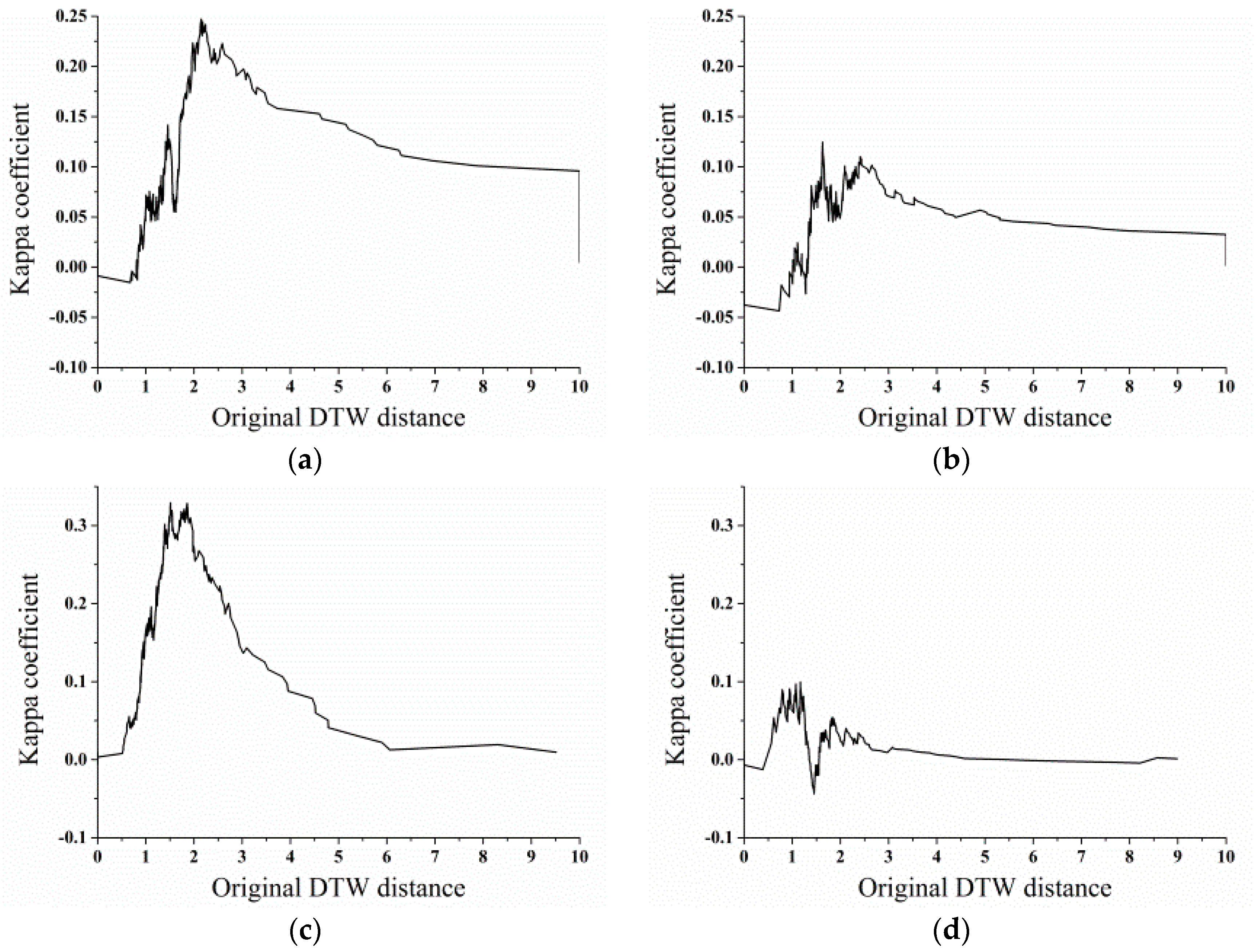
For the OLWDTW method, the major problem is selecting the σ 
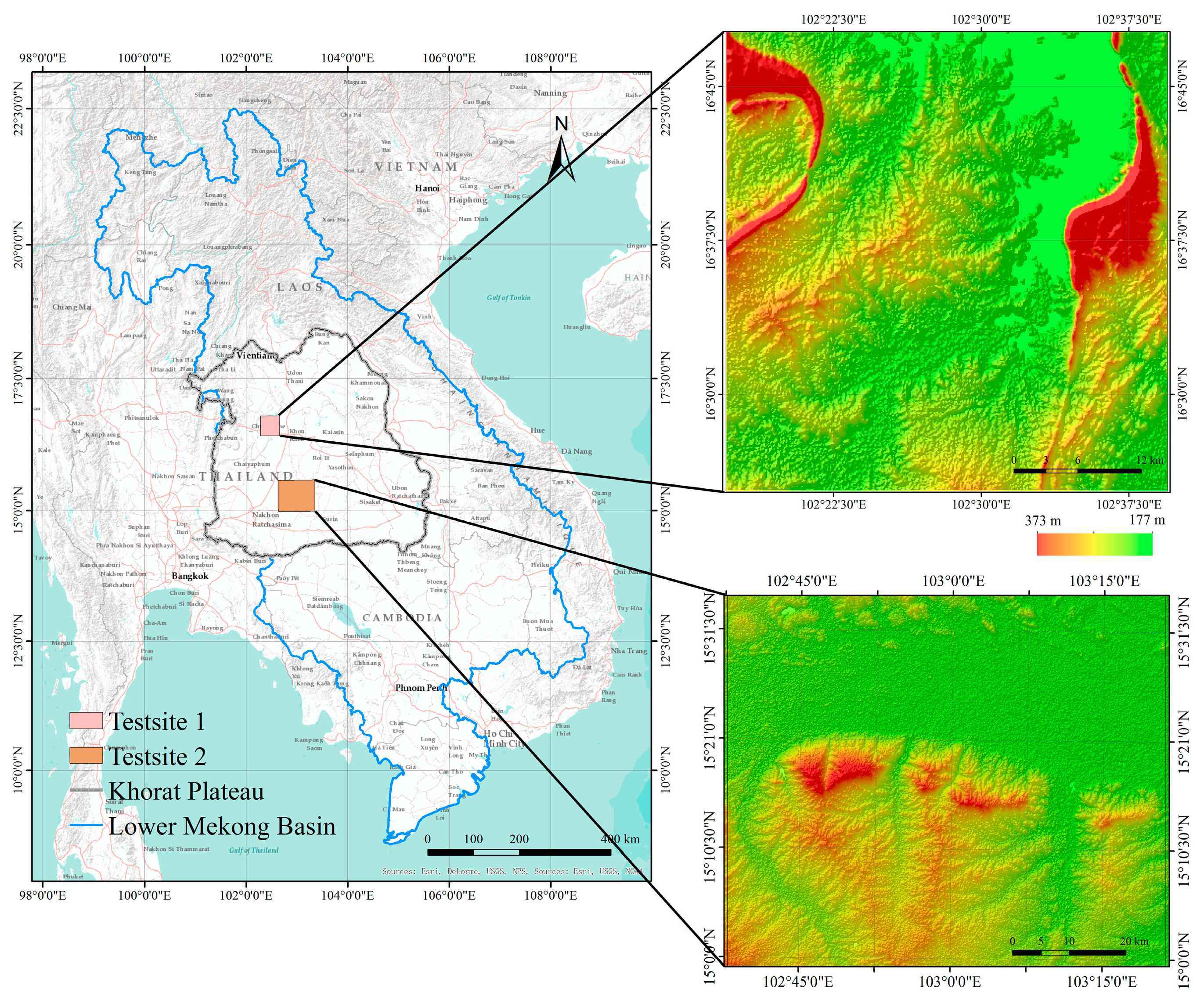
value to achieve the highest classification accuracy. In this paper, we repeatedly tested the performance of OLWDTW under different σ values for 300 sample points in test site 1 and 300 sample points in test site 2, using the sample points to obtain the distance of the pixel’s NDVI time series with the reference NDVI time series. The performance is evaluated by the kappa coefficient. This step is to obtain the value of σ and use this parameter to achieve the highest classification accuracy of cropland by the OLWDTW method. The kappa coefficient was defined as the proportion of agreements between paired observations, corrected for chance agreement as estimated from the marginal frequencies over the K response categories [38,39]. The equation to calculate the kappa coefficient is shown in Equation (4):
k = p 0 p c 1 p c
where p 0 is the observed agreement and p c is the chance agreement.
Calculation of the observed agreement p 0 is shown in Equation (5). Calculation of the chance agreement p c is shown in Equation (6):
p 0 = a + d n
p c = ( ( a + c ) × ( a + b ) n ) + ( ( b + d ) × ( c + d ) n ) n
where n is the total number of observations, a is the number of agreements of observation 1 and observation 2 on a positive category, b is the number of agreements of observation 1 and observation 2 on a negative category, c is the number of negative category of observation 1 but positive category on observation 2, d is the number of positive category of observation 1 but negative category on observation 2 and as shown in Table 2.
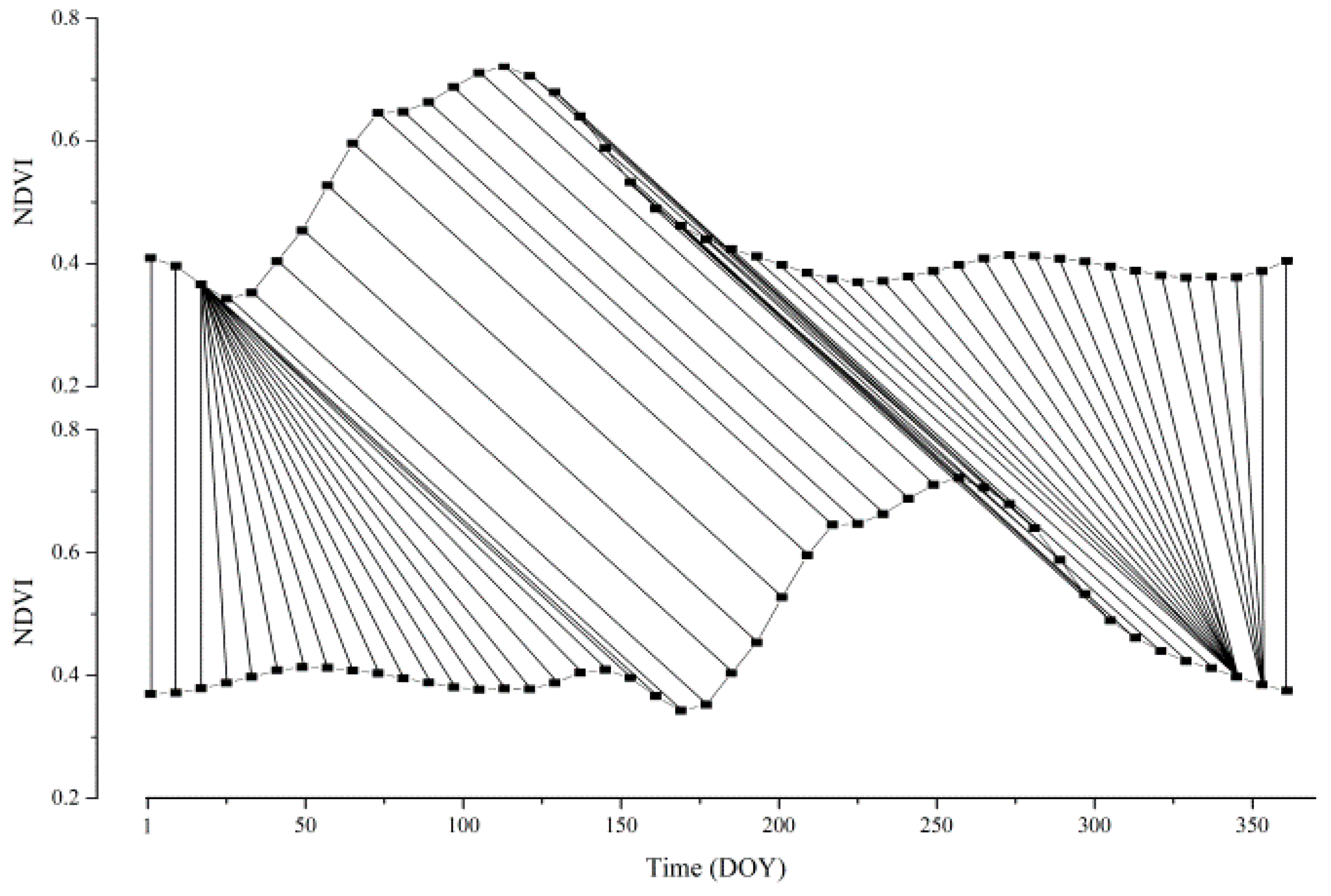
Before explaining how to select the parameter σ , we should first explain how to select the threshold on the similarity measure map to obtain the highest classification accuracy. The method is simple. It first compares the similarity between each pixel’s NDVI time series with the reference NDVI time series using the ODTW/OLWDTW distance method. The lower the value of the distance between a pixel’s NDVI time series with the reference NDVI time series, the more likely the pixel is to belong to the land cover type of the reference NDVI time series. The second step of our method is to select a threshold value. Those pixels with distance values higher than the threshold are considered to not belong to the cropland type of the reference NDVI time series. Those pixels with distance values lower than the threshold are considered to belong to the cropland type of the reference NDVI time series so that when we select the threshold value, it guarantees the highest kappa coefficient value. The threshold is obtained in three steps:
  • Arrange the randomly selected sample points by distance to the reference NDVI time series.
  • Calculate the kappa coefficient by hypothesizing the threshold from the first value arranged in the distance list to the last value of the distance.
  • Ensure the threshold value brings the highest kappa coefficient.
As shown in Table 3, assume that 10 sample points are randomly selected. They have two attributes. The first is the true classification of whether the pixel belongs to the crop type of the reference NDVI time series (“True classification” in the first column in Table 3). The second attribute is the distance between the pixels’ NDVI time series and the reference NDVI time series (“Distance value” in the second column in Table 3). Threshold is the distance value to be used. For example, if the threshold value is 0.99, then the threshold classification result value at 0.99 is 0 (“Threshold classification result” in the third column in Table 3) and the rest of the distance value is 1. Then the first row is correctly classified (the true classification result is 0 and the classification result with a threshold distance of 0.99 is 0), while the second row is misclassified because the true classification result is 0 and the classification result with distance value 0.99 is 1. Thus, the third row, sixth row, seventh row, ninth row and tenth row are correctly classified. The second row, fourth row, fifth row and eighth row are misclassified. Then according to Equation (4), the kappa coefficient value is 0. If the threshold value is 1.17, then the threshold classification result value of 0.99 and in 1.17 is 0 and the remaining distance value is 1. The kappa coefficient is 0.2 and so on. In Table 3, when the threshold distance value is 1.52, the kappa coefficient reached its highest value of 0.6 so the threshold we use is 1.52.
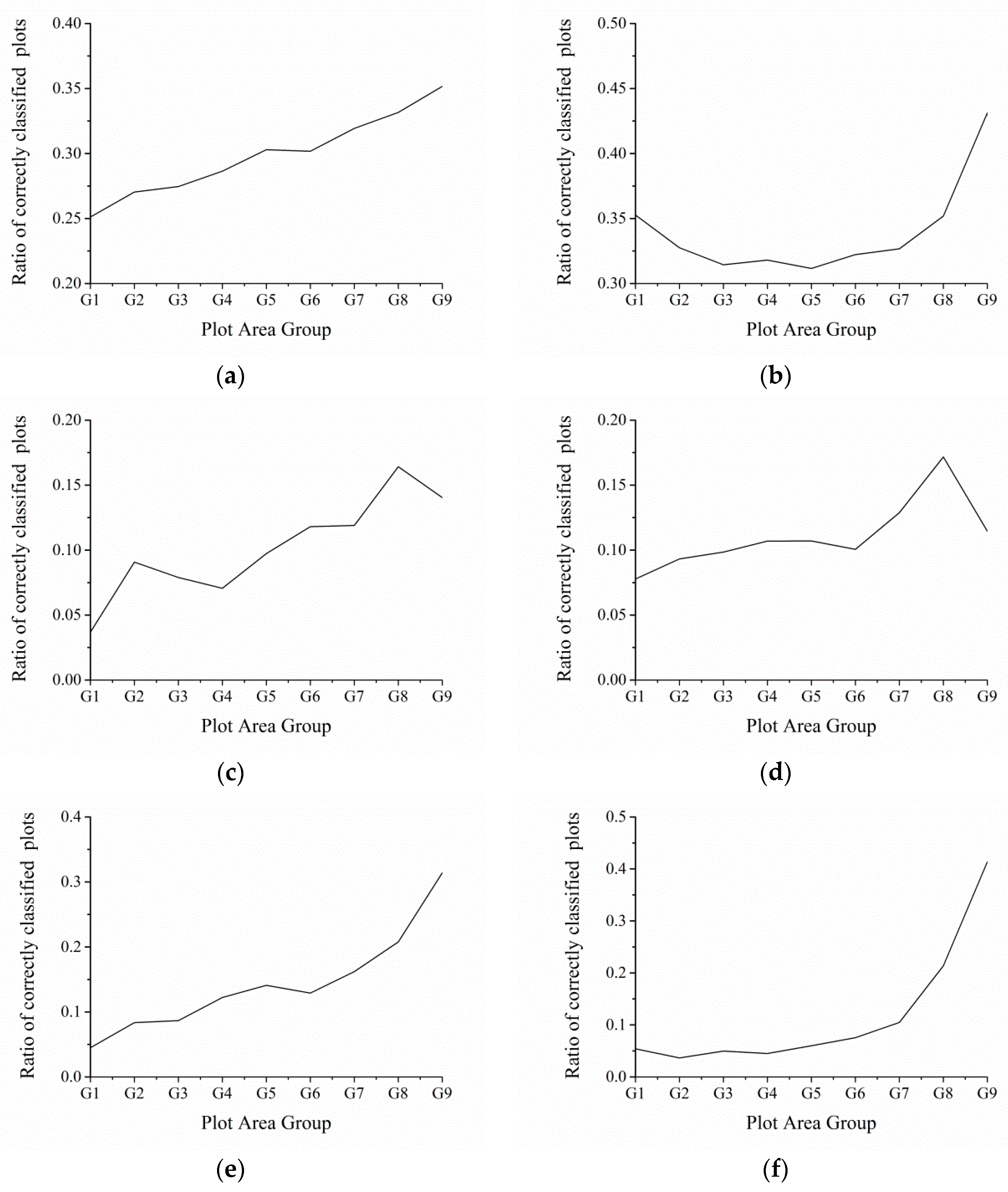
Obtaining the value of σ achieves the highest cropland classification accuracy using the OLWDTW method. We tested values from 1.5 to 5 and increased by 0.5. Selecting the highest kappa coefficient then selecting the value of σ resulted in the highest kappa coefficient.

3. Results and Discussion

The flow of the experiment to test OLWDTW is shown in Figure 4. First, we obtained the reference annual NDVI time series of rice paddy fields and dryland crops. Secondly, we used the DTW algorithm and OLWDTW algorithm to calculate the distance between each pixel’s NDVI time series with the reference NDVI time series. In terms of the OLWDTW method, a parameter value of σ was tested for the best extraction accuracy for cropland. Finally, we obtained the threshold of the time-series distance. The pixels with a time-series distance higher than the threshold are rejected because the NDVI time series are not similar to the reference NDVI time series.

3.1. Classification by Original DTW Method

To test the effectiveness of our method, we extracted the rice paddy field and dryland crop field in the two test sites and verified the extraction accuracy using the validation classification map. We first used 277 sample points on the validation classification map to obtain the reference annual NDVI time series of rice paddy fields and dryland fields.
We obtained the distance between each pixel’s NDVI time series and the reference NDVI time series using the original DTW distance. In order to obtain the highest classification accuracy, according to the threshold value selection described in Section 2.3.3, we obtained the threshold to extract the four crop types. We randomly selected 300 sample points from the validation classification map. Because the validation classification map only has the rice paddy and dryland crop types, the single cropping rice was combined with double cropping rice. The dryland crop 1 should be combined with dryland crop 2. We used a max-min operation to combine the four crop types, namely selecting the smaller value of the distance on a pixel. The two combined types of croplands were the rice paddy and dryland.
From the 300 randomly selected points, we observed that as the threshold of the original DTW distance grew, the kappa coefficient values changed. As shown in Figure 5, the kappa coefficient reached a peak value of 0.247 for the rice paddy type. The corresponding original DTW distance value was 2.15. The kappa coefficient reached a peak value of 0.123 for dryland crop cover. The corresponding original DTW distance value was 1.63. In test site 2, the kappa coefficient reached a peak value of 0.329 for rice paddy cover. The corresponding original DTW distance value was 1.51. The kappa coefficient reached a peak value of 0.099 for dryland crops. The corresponding original DTW distance value was 1.17. Thus, for test site 1, the threshold DTW distances to the extracted cropland types of rice paddy and dryland crop were 2.15 and 1.63. In test site 2, the threshold DTW distances to the extracted cropland types of rice paddy and dryland crop were 1.51 and 1.17.

3.2. Classification with the OLWDTW Method

3.2.1. Selecting σ Values

Using the method introduced in Section 2.3.3, we tested the optimal threshold to extract cropland by original DTW distance. Here we review the three steps for threshold selection using an example. Assuming that 100 points are randomly selected based on the validation map, the first step is to overlap the 100 points on the rice paddy class’ distance map produced by the ODTW method or OLWDTW method. As we know from the principle of the ODTW and OLWDTW methods, the smaller the value of the ODTW or OLWDTW distance, the more likely the pixel is to belong to rice paddies. We need to decide on the threshold of the distance value so that if the pixel’s ODTW or OLWDTW distance exceeds the threshold, it is judged to not belong to the rice paddy class because the remote sensing time series is dissimilar to the reference rice paddy remote sensing time series. By overlapping the 100 points on the rice paddy class’ distance map, we can obtain the distance value of the 100 points with the reference rice paddy remote sensing time series. In the second step, we arrange the 100 points by their distance values, as shown in the second column of Table 3. Now we obtain two attributes for the 100 randomly selected points, whether the points belong to rice paddies (from the validation map) and the distance value of the points’ remote sensing time series to the reference rice paddy remote sensing time series. In the third step, we test the threshold by selecting the threshold value from the first arranged point’s distance value to the last point’s distance value. In the final step, we take the threshold when the kappa coefficient reaches its highest value. Taking an extreme example, there is only one point among the 100 points where the rice paddy class and the ODTW or OLWDTW distance value of that point’s remote sensing time series to the reference rice paddy remote sensing time series is 0.01. The rest of the points’ distance values are greater than 0.01. We know that if we take the threshold as 0.01, the kappa coefficient reaches its peak, because when we take other distance values as the threshold, the kappa coefficient is lower than the peak. Similar to a practical application, the experiment was on all threshold values and calculated the kappa coefficient until it reached its peak.
For OLWDTW distance, the extraction accuracy for cropland is affected by a different enhance factor of the σ value. Therefore, before selecting threshold values, the enhance factor of the σ value should first be determined. As we introduced in Section 2.3.3, we tested the value of σ from 1.5 to 5 and increased by 0.5, selecting the highest kappa coefficient corresponding to the σ value as the final enhance factor value. The optimal enhance factor σ for OLWDTW distance was obtained by testing different kappa coefficients with different σ values for rice paddies in test site 1. OLWDTW distances with different σ for rice paddies are shown in Figure 6.
To evaluate which value of σ yielded the highest performance with the OLWDTW, the relationship of the kappa coefficient with OLWDTW at different σ values is shown in Figure 7. The method is similar to the method in which we determined the threshold values for the original DTW distance. Figure 7 shows the maximum kappa coefficient value under different enhance factor σ. Table 4 lists the specific values.
We picked a σ value of 4.5 and OLWDTW threshold of 4.39 to classify the rice paddy type in test site 1.
A similar operation was conducted with the the dryland crop in test site 1 and the rice paddy and dryland crop in test site 2. Using the 600 sample points in test site 1 and test site 2, the value of σ and the highest kappa coefficient of the corresponding OLWDTW distance were calculated. The highest kappa coefficient value the OLWDTW method could achieve with different σ values is shown in Table 5 and Table 6.
From Table 5 and Table 6, we obtain the most suitable enhance factor σ value and the corresponding extraction threshold. With the optimal threshold and enhance factor σ, cropland distribution is ready to be drawn by DTW and the OLWDTW method.

3.2.2. OLWDTW Distance

Using the enhance factor σ with the highest kappa coefficient value, we could obtain the OLWDTW distance in test site 1 and test site 2. According the steps conducted in Section 3.2.1, in test site 1, the enhance factor σ values for rice paddy and dryland crop were determined as 4.5 and 3. In test site 2, the enhance factor σ values for rice paddy and dryland crop 1 and dryland were determined as 1.5 and 5. In Figure 8, the OLWDTW distances with the selected enhance factor σ for each crop type are illustrated.
Using the threshold value to extract each cropland type would create separate crop distribution maps, and the separate crop distribution maps might overlap. The original DTW distance method generated overlapping layers, so we decided the final cropland type using the DTW distance. The lower DTW distance of the overlapping layer was decided as the final class type. For the OLWDTW distance, because different enhance factor σ values from overlapping layers produced uneven threshold values, we decided the final class of the overlapping layer by the layer with the highest kappa coefficient.

3.3. Cropland Classification and Accuracy Assessment

3.3.1. Cropland Distribution Mapping

The similarity measure of each pixel’s annual NDVI time series with the reference NDVI time series was obtained using the original DTW distance and the OLWDTW distance. The threshold we obtained from Section 3.1 and Section 3.2.1 was used to extract the two crop types in the two test sites. For the overlapping region, the lower DTW distance was decided as the final class type. Figure 9 shows the distribution of dryland and rice paddy in test 1 and test 2 classified by the ODTW and OLWDTW methods before combination and dealing with the overlapping region. For the OLWDTW distance, we decided the final class of the overlapping layer by the layer with the highest kappa coefficient. The final cropland distribution is shown in Figure 9.

3.3.2. Accuracy Assessment and Comparisons

We used validation classification maps provided by the Land Development Department at the Office of Soil Resources Survey and Research. The classification system of this dataset on level 1 includes five classes, namely urban and built-up land, agricultural land, forest land, water body and miscellaneous land. The classification system for level 2 of agricultural land and the area of each class is shown in Table 7.
We used the paddy field class to verify the classification of our rice paddy class’ accuracy. The field crop class in the validation classification map was used to verify the dryland crop class’ classification accuracy. Note that the annual growth patterns of perennial crops are more similar to woodland rather than dryland crops, so the field crops were used for validation of the dryland crops. The distribution of the paddy field class and dryland crop class in the validation classification map is shown in Figure 10.
We first quantitatively tested our extraction results. The areas of dryland crop and rice paddy extracted by the original DTW distance method and OLWDTW method and the validation land cover map are shown in Table 8.
We can see from Table 9 that in test site 1, the OLWDTW-extracted rice paddy area is slightly closer to the validation land cover map. But the dryland crop area is closer using the ODTW method. While the ODTW underestimated rice paddy area in test site 2 by 548.61 km2 the OLWDTW method provided a closer estimate, overestimating the area by 10.33 km2. We also used the validation classification map to verify the classification results of our method using a confusion matrix, as shown in Table 9, Table 10, Table 11 and Table 12.
The overall accuracies of the ODTW and OLWDTW classification results in test site 1 and test site 2 were 51.30%, 56.48%, 52.17% and 59.85%. The overall accuracy of OLWDTW exceeded the ODTW method by 5.18% and 7.68% in test 1 and test 2. The kappa coefficients of the two methods in the two test sites were 0.234, 0.297, 0.196 and 0.264. It can be seen from Figure 10 that the OLWDTW classification results of dryland crops in test site 1 and test site 2 are worse, but the overall accuracy tested by the validation map is accurate. This is because the proportion of dryland crop area is low. Therefore, the misclassification result of dryland crops did not have much if an effect on the overall classification accuracy. The classification results of OLWDTW were spatially more consistent with the validation classification map than the ODTW method in terms of the overall accuracy. In terms of the individual class, the producer’s accuracy and user’s accuracy of the rice paddy and dryland crop classes in test 1 and test 2 classified by the ODTW and OLWDTW methods are shown in Table 13.
As shown in Table 13, for rice paddy, the classification producer’s accuracy and user’s accuracy using the OLWDTW method are higher than the ODTW method in both test sites. In terms of dryland crops, the producer’s accuracy of the OLWDTW method is higher than the ODTW method in the two test sites, but the user’s accuracy of the OLWDTW method is lower than producer’s accuracy in the two test sites. In conclusion, overall classification accuracies of cropland obtained by the ODTW and OLWDTW methods in test site 1 were 51.30% and 56.48%. In test site 2, the overall classification accuracies of cropland obtained by ODTW and OLWDTW were 52.17% and 59.85%. In terms of the single crop type classification performance, the producer’s accuracy values of the rice paddy class obtained by ODTW and OLWDTW in test site 1 and test site 2 were 69.92%, 77.51%, 58.66% and 73.31%. User’s accuracy values of rice paddy obtained by ODTW and OLWDTW in test site 1 and test site 2 were 44.78%, 50.97%, 71.36% and 73.07%. The performance of OLWDTW in the classification of rice paddies was satisfactory. As for the dryland crop, the producer’s accuracy values of dryland crops obtained by ODTW and OLWDTW in test site 1 and test site 2 were 19.11%, 9.53%, 27.87% and 15.49%. The user’s accuracy values of dryland crops obtained by ODTW and OLWDTW in test site 1 and test site 2 were 27.27%, 28.52%, 20.01% and 24.76%.

3.4. Discussion

The DTW-based method has already received attention from researchers for recognizing similarity in remote sensing time-series data. However, the original DTW method gives the same weight to all the points in the time series. Our research proves that properly enhancing the weighting factor of growth season sections in the annual NDVI time series can help improve the classification accuracy of identifying cropland. It is shown in the experiment results that OLWDTW achieved a higher overall accuracy in cropland and rice paddy classification than the original DTW method. The OLWDTW resulted in higher overall accuracy on cropland classification than the ODTW distance value because the OLWDTW method is more logically and practically suitable for crop extraction. When the original DTW distance method was applied to the extraction of crops, the annual remote sensing time series were equally weighted for the similarity measure. However, the shape of remote sensing time series in the growing period of crops was more important for crop recognition. Therefore, adding a proper weight on the growth section of the annual remote sensing time series when extracting crop distributions using the ODTW method can improve the classification accuracy. This paper presents this method and experiment for deciding the proper weight values. The two experiments proved that OLWDTW is superior to the ODTW method in terms of extracting cropland distributions. However, some problems also appeared in the experiment results. The user’s accuracy of dryland crop when using the OLWDTW method had a lower value than the extraction results of the original DTW method.
We tested the proposed OLWDTW method in two test sites in Khorat Plateau, near the Mekong River. As shown in Figure 8, we examined the classification accuracy of the OLWDTW method and compared it with the classification accuracy of ODTW with a quantitative method. It can be seen from the extracted area validation that the OLWDTW performs better on the extraction of rice paddy fields. However, OLWDTW underestimated the area of dryland crops in the two test sites. Quantitative comparison with the area extracted by the ODTW method showed that the ODTW performed better when extracting dryland crops in test site 1, but OLWDTW performed better than ODTW in test site 2. Spatial validation of the performance of OLWDTW was also conducted. The spatial validation results of the OLWDTW method were also compared with the ODTW method. The result shows that the overall accuracy of OLWDTW exceeded the ODTW method by 5.18% and 7.68% in test 1 and test 2. In terms of the single crop type classification performance, the performance of OLWDTW in the classification of rice paddies was more satisfactory than the ODTW method. As for the dryland crop, OLWDTW performed better than the ODTW method in terms of the producer’s accuracy in the two test sites. However, the user’s accuracy of dryland crops obtained by OLWDTW was lower than the ODTW method. The better performance on the producer’s accuracy but worse performance on the user’s accuracy when extracting dryland crops with OLWDTW, as well as the underestimated area of dryland crops, means that the dryland crops extracted using the OLWDTW method were more correct than the results of the ODTW method. The worse performance on the user’s accuracy when extracting dryland crops was caused by many dryland crop plateaus being replaced by the rice paddy class’ plateau because the kappa coefficient of the dryland crop class was lower than that of the rice paddy class. This led to many misclassifications of dryland crop with the OLWDTW method. In order to get the highest overall accuracy with OLWDTW, we directly replaced dryland crops with rice paddy fields. This caused the problem of underestimating the area of dryland crops. This is a hint that the method for combining overlapping regions of the OLWDTW method needs to be changed and improved.
The validation classification map is a manually interpreted map. Therefore, it is fragmented, reflecting the small plot size of dryland crops and rice paddies. The fragmented plot size of the validation classification map led to a low overall classification accuracy for the ODTW and OLWDTW methods based on the 250-m MODIS time-series data, particularly for the dryland crops. We have illustrated the plot size provided by validation classification map in Section 2.1. It can be seen that the plot size of dryland crops is lower than that of the rice paddies. This could be a reason for the lower classification accuracy of dryland crops. In order to test the effect on classification accuracy of plot size in the validation classification map, we analyzed the correlation between the classification accuracy of the OLWDTW method with the plot size of the validation classification map. First, we divided the plot size into nine groups according to the area: (0 km2–0.01 km2), (0.01 km2–0.02 km2), (0.02 km2–0.03 km2), (0.03 km2–0.04 km2), (0.04 km2–0.065 km2), (0.065 km2–0.1 km2), (0.1 km2–0.5 km2), (0.5 km2–1 km2), and (1 km2–1000 km2). Each group had roughly the same number of plots. Second, we calculated statistics for the overall accuracy, rice paddy classification accuracy, and dryland crop classification accuracy in each plot size group. The statistical method was to count the mean plot numbers in each group of correctly classified results and misclassified results. For example, we calculating the overall classification accuracy of cropland in the first group. Suppose there is a total of 2000 plots among the first group, 1500 plots were misclassified and 500 plots were correctly classified, then the mean number of misclassified plots in the first group would be 0.75 and the mean number of correctly classification plots in the first group would be 0.25. Using this method, we can clearly determine the relationship between plot size and classification accuracy as shown in Figure 11, which demonstrates that the trend of the ratio of correctly classified plots increases as the plot sizes become larger. This is because MODIS NDVI time-series data have a low to moderate spatial resolution. If the plot sizes were smaller than MODIS NDVI pixels, mixed pixels would exist and create a chaotic shape beyond the recognition capabilities of the OLWDTW method. According to the validation classification map, the mean plot size of the rice paddies was 0.5 km2 in test site 1 and 1.46 km2 in test site 2. The mean plot size of the dryland crop in test site 1 was 0.14 km2 and 0.15 km2 in test site 2. A total of 11.84% of dryland crop plots in test site 1 were smaller than the MODIS pixel size, while only 2.82 percent of rice paddy sizes in test site 1 were lower than the MODIS pixel size. A total of 10.75 percent of dryland crop plots in test site 2 were smaller than the MODIS pixel size. Only 0.86 percent of dryland crop plots in test site 2 were smaller than the MODIS pixel size. The smaller plot sizes explain the lower classification accuracy of dryland crops compared to rice paddies.
Proper selection of a weighting factor value σ is important for the application of the OLWDTW distance method. In this paper, before introducing the selection of value σ, we discussed an avenue to obtain the threshold for the ODTW method. In the process of selecting a threshold for the ODTW method, a sufficient quantity of sample points was required. In this paper, we randomly selected the rice paddies or dryland crop points on the validation map. However, in a realistic condition, the sample points should be obtained by a field survey or by sampling a high-resolution remote sensing image. We suggest using randomly distributed sampling data on the map. Mixed pixels should also be included in the sampling points because in a realistic situation, mixed pixels are exists The method to select the threshold value for ODTW also provides a novel method for the threshold selection scheme in the time-series similarity measure-based approaches using remote sensing classification. Our research proves that the weighting factor value σ is not fixed for one curve in different regions. Therefore, we should carefully select abundant and evenly distributed sampling points for local weight values when classifying large areas of cropland.
Because our method is based on threshold extraction, after the cut-off of the threshold OLWDTW distance operation, different classes might produce overlapping regions. For the original DTW distance method, we can simply decide on the class that has a lower DTW distance value. However, according to our test, the same curve’s enhance factor is not identical in different testing locations. The OLWDTW-based time series similarity is not easy to unify with scales of the distance value using different enhance factor values. For the OLWDTW method, the major problem was to dealing with the overlapping regions of different classes. The OLWDTW method obtained higher overall classification accuracy for the cropland and rice paddy types, but obtained lower user’s classification accuracy on dryland crops. This was caused by the immature combination algorithm. Future work should improve on the problem of combining the overlapping regions. The current method for dealing with the overlapping region with the OLWDTW method is to replace crops with a lower kappa coefficient with crops with a higher kappa coefficient. This is based on the global classification accuracy. A possible solution to improve the overall accuracy is to develop a local classification accuracy and decide which crop type to retain using the local classification accuracy rather than the global accuracy. This is an information combination method. Local classification accuracy could be based on the entropy of fuzzy classification results, as studied by Fauvel et al. [40]. The entropy-based local classification accuracy would not be affected by the different weighting factors.

4. Conclusions

This article applied an open-boundary locally weighted dynamic time warping distance method developed for the recognition of cropland in Southeast Asia. The OLWDTW distance algorithm was developed based on the DTW distance. An enhancement factor was added to the original DTW among the growth season section of the annual NDVI time series that allowed for strengthening the affection of the growth season section when comparing the annual NDVI time series’ similarities. In the study area within the Lower Mekong Delta in Southeast Asia, the method was proven to achieve higher overall accuracy for mapping cropland distribution. Although the overall accuracy of cropland classification was higher than the original DTW distance, the classification accuracy of dryland crops was worse than the original DTW distance. This was caused by the small plot size of dryland crops and an inappropriate method for dealing with the overlapping region.
Two test areas were selected to verify the approach. The overall accuracy of cropland extraction improved by about 5% and 7% in the two test sites compared to ODTW. The results highlight the potential of OLWDTW to improve the classification accuracy of rice paddies, but for dryland crops further work is needed to obtain a higher classification accuracy. We expect that the OLWDTW algorithm will be used for large-scale cropland classification of remote sensing time-series data after a better technique is developed to deal with overlapping regions of croplands. However, classifying one kind of crop, especially rice paddies, over large areas is feasible in the current version.

Acknowledgments

This research was supported by the National Natural Science Foundation of China under grants 41661144030, 41471335, 41561144012, 41671422, 41501430; the Innovation Project of LREIS under grant O88RA303YA; and the National Science-Technology Support Plan Projects under grant 2013BAD05B03.

Author Contributions

Gaohuan Liu conceived the study. Xudong Guan performed the data analysis and wrote the paper. Chong Huang and Qingsheng Liu supervised and provided logistical support to the research. Xuelian Meng provided feedback on the study design and modified the manuscript. Chunsheng Wu and Xiare Pati helped in the data processing. Zhuoran Chen and Qiang Wang improved the program for the OLWDTW method. All authors reviewed and approved the manuscript.

Conflicts of Interest

The authors declare no conflict of interest.

References

  1. Kuenzer, C.; Knauer, K. Remote sensing of rice crop areas. Int. J. Remote Sens. 2013, 34, 2101–2139. [Google Scholar] [CrossRef]
  2. Pittman, K.; Hansen, M.C.; Becker-Reshef, I.; Potapov, P.V.; Justice, C.O. Estimating global cropland extent with multi-year modis data. Remote Sens. 2010, 2, 1844–1863. [Google Scholar] [CrossRef]
  3. Xiao, X.; Boles, S.; Frolking, S.; Li, C.; Babu, J.Y.; Salas, W.; Moore, B. Mapping paddy rice agriculture in south and southeast Asia using multi-temporal MODIS images. Remote Sens. Environ. 2006, 100, 95–113. [Google Scholar] [CrossRef]
  4. Cheng, T.; Yang, Z.W.; Inoue, Y.; Zhu, Y.; Cao, W.X. Preface: Recent advances in remote sensing for crop growth monitoring. Remote Sens. 2016, 8, 116. [Google Scholar] [CrossRef]
  5. Idso, S.B.; Jackson, R.D.; Reginato, R.J. Remote-sensing of crop yields. Science 1977, 196, 19–25. [Google Scholar] [CrossRef] [PubMed]
  6. Azzari, G.; Jain, M.; Lobell, D.B. Towards fine resolution global maps of crop yields: Testing multiple methods and satellites in three countries. Remote Sens. Environ. 2017, 202, 129–141. [Google Scholar] [CrossRef]
  7. Nguyen, D.B.; Clauss, K.; Cao, S.M.; Naeimi, V.; Kuenzer, C.; Wagner, W. Mapping rice seasonality in the Mekong delta with multi-year envisat ASAR WSM data. Remote Sens. 2015, 7, 15868–15893. [Google Scholar] [CrossRef] [Green Version]
  8. Sakamoto, T.; Yokozawa, M.; Toritani, H.; Shibayama, M.; Ishitsuka, N.; Ohno, H. A crop phenology detection method using time-series MODIS data. Remote Sens. Environ. 2005, 96, 366–374. [Google Scholar] [CrossRef]
  9. Xiao, X.M.; Boles, S.; Liu, J.Y.; Zhuang, D.F.; Frolking, S.; Li, C.S.; Salas, W.; Moore, B. Mapping paddy rice agriculture in southern China using multi-temporal MODIS images. Remote Sens. Environ. 2005, 95, 480–492. [Google Scholar] [CrossRef]
  10. Blaes, X.; Vanhalle, L.; Defourny, P. Efficiency of crop identification based on optical and SAR image time series. Remote Sens. Environ. 2005, 96, 352–365. [Google Scholar] [CrossRef]
  11. Moody, A.; Johnson, D.M. Land-surface phenologies from AVHRR using the discrete fourier transform. Remote Sens. Environ. 2001, 75, 305–323. [Google Scholar] [CrossRef]
  12. Murakami, T.; Ogawa, S.; Ishitsuka, N.; Kumagai, K.; Saito, G. Crop discrimination with multitemporal SPOT/HRV data in the saga plains, Japan. Int. J. Remote Sens. 2001, 22, 1335–1348. [Google Scholar] [CrossRef]
  13. Fensholt, R.; Proud, S.R. Evaluation of earth observation based global long term vegetation trends—Comparing GIMMS and MODIS global NDVI time series. Remote Sens. Environ. 2012, 119, 131–147. [Google Scholar] [CrossRef]
  14. Gong, P.; Wang, J.; Yu, L.; Zhao, Y.C.; Zhao, Y.Y.; Liang, L.; Niu, Z.G.; Huang, X.M.; Fu, H.H.; Liu, S.; et al. Finer resolution observation and monitoring of global land cover: First mapping results with Landsat TM and ETM+ data. Int. J. Remote Sens. 2013, 34, 2607–2654. [Google Scholar] [CrossRef]
  15. Liao, T.W. Clustering of time series data—A survey. Pattern Recognit. 2005, 38, 1857–1874. [Google Scholar] [CrossRef]
  16. Pena-Barragan, J.M.; Ngugi, M.K.; Plant, R.E.; Six, J. Object-based crop identification using multiple vegetation indices, textural features and crop phenology. Remote Sens. Environ. 2011, 115, 1301–1316. [Google Scholar] [CrossRef]
  17. Sakamoto, T.; Van Nguyen, N.; Kotera, A.; Ohno, H.; Ishitsuka, N.; Yokozawa, M. Detecting temporal changes in the extent of annual flooding within the Cambodia and the Vietnamese Mekong delta from MODIS time-series imagery. Remote Sens. Environ. 2007, 109, 295–313. [Google Scholar] [CrossRef]
  18. Rembold, F.; Atzberger, C.; Savin, I.; Rojas, O. Using low resolution satellite imagery for yield prediction and yield anomaly detection. Remote Sens. 2013, 5, 1704–1733. [Google Scholar] [CrossRef] [Green Version]
  19. Xiong, J.; Thenkabail, P.S.; Gumma, M.K.; Teluguntla, P.; Poehnelt, J.; Congalton, R.G.; Yadav, K.; Thau, D. Automated cropland mapping of continental Africa using google earth engine cloud computing. ISPRS J. Photogramm. Remote Sens. 2017, 126, 225–244. [Google Scholar] [CrossRef]
  20. Xiong, J.; Thenkabail, P.; Tilton, J.; Gumma, M.; Teluguntla, P.; Oliphant, A.; Congalton, R.; Yadav, K.; Gorelick, N. Nominal 30-m cropland extent map of continental Africa by integrating pixel-based and object-based algorithms using Sentinel-2 and Landsat-8 data on google earth engine. Remote Sens. 2017, 9, 1065. [Google Scholar] [CrossRef]
  21. Gumma, M.K.; Thenkabail, P.S.; Teluguntla, P.; Rao, M.N.; Mohammed, I.A.; Whitbread, A.M. Mapping rice-fallow cropland areas for short-season grain legumes intensification in South Asia using MODIS 250 m time-series data. Int. J. Digit. Earth 2016, 9, 981–1003. [Google Scholar] [CrossRef] [Green Version]
  22. Tan, P.; Lymburner, L.; Thankappan, M.; Lewis, A. Mapping cropping practices using MODIS time series: Harnessing the data explosion. J. Indian Soc. Remote Sens. 2011, 39, 365–372. [Google Scholar] [CrossRef]
  23. Bagan, H.; Wang, Q.; Yang, Y.; Yasuoka, Y.; Bao, Y. Land cover classification using moderate resolution imaging spectrometer-enhanced vegetation index time-series data and self-organizing map neural network in inner Mongolia, China. J. Appl. Remote Sens. 2007, 1, 013545. [Google Scholar] [CrossRef]
  24. Geerken, R.; Zaitchik, B.; Evans, J.P. Classifying rangeland vegetation type and coverage from NDVI time series using fourier filtered cycle similarity. Int. J. Remote Sens. 2005, 26, 5535–5554. [Google Scholar] [CrossRef]
  25. Gorecki, T.; Luczak, M. Multivariate time series classification with parametric derivative dynamic time warping. Expert Syst. Appl. 2015, 42, 2305–2312. [Google Scholar] [CrossRef]
  26. Aghabozorgi, S.; Shirkhorshidi, A.S.; Teh Ying, W. Time-series clustering—A decade review. Inf. Syst. 2015, 53, 16–38. [Google Scholar] [CrossRef]
  27. Petitjean, F.; Inglada, J.; Gancarski, P. Satellite image time series analysis under time warping. IEEE Trans. Geosci. Remote Sens. 2012, 50, 3081–3095. [Google Scholar] [CrossRef]
  28. Petitjean, F.; Kurtz, C.; Passat, N.; Gancarski, P. Spatio-temporal reasoning for the classification of satellite image time series. Pattern Recognit. Lett. 2012, 33, 1805–1815. [Google Scholar] [CrossRef]
  29. Weber, J.; Petitjean, F.; Ganarski, P. Towards efficient satellite image time series analysis: Combination of dynamic time warping and quasi-flat zones. In Proceedings of the 2012 IEEE International Geoscience and Remote Sensing Symposium, Munich, Germany, 22–27 July 2012; pp. 4387–4390. [Google Scholar]
  30. Guan, X.D.; Huang, C.; Liu, G.H.; Meng, X.L.; Liu, Q.S. Mapping rice cropping systems in Vietnam using an NDVI-based time-series similarity measurement based on DTW distance. Remote Sens. 2016, 8, 19. [Google Scholar] [CrossRef]
  31. Maus, V.; Câmara, G.; Cartaxo, R.; Sanchez, A.; Ramos, F.M.; Queiroz, G.R.d. A time-weighted dynamic time warping method for land-use and land-cover mapping. IEEE J. Sel. Top. Appl. Earth Obs. Remote Sens. 2016, 9, 3729–3739. [Google Scholar] [CrossRef]
  32. Cosslett, T.L.; Cosslett, P.D. Introduction. In Sustainable Development of Rice and Water Resources in Mainland Southeast Asia and Mekong River Basin; Springer: Singapore, 2018; pp. 1–4. [Google Scholar]
  33. U.S. Department of the Interior; U.S. Geological Survey. MOD09Q1|LP DAAC: NASA Land Data Products and Services. Available online: https://lpdaac.usgs.gov/dataset_discovery/modis/modis_products_table/mod09q1_v006 (accessed on 14 February 2016).
  34. Jönsson, P.; Eklundh, L. Timesat—A program for analyzing time-series of satellite sensor data. Comput. Geosci. 2004, 30, 833–845. [Google Scholar] [CrossRef]
  35. Fensholt, R.; Rasmussen, K.; Nielsen, T.T.; Mbow, C. Evaluation of earth observation based long term vegetation trends—Intercomparing NDVI time series trend analysis consistency of Sahel from AVHRR GIMMS, TERRA MODIS and SPOT VGT data. Remote Sens. Environ. 2009, 113, 1886–1898. [Google Scholar] [CrossRef]
  36. Petitjean, F.; Ketterlin, A.; Gancarski, P. A global averaging method for dynamic time warping, with applications to clustering. Pattern Recognit. 2011, 44, 678–693. [Google Scholar] [CrossRef]
  37. Sakoe, H.; Chiba, S. Dynamic-programming algorithm optimization for spoken word recognition. IEEE Trans. Acoust. Speech Signal Process. 1978, 26, 43–49. [Google Scholar] [CrossRef]
  38. Viera, A.J.; Garrett, J.M. Understanding interobserver agreement: The kappa statistic. Fam. Med. 2005, 37, 360–363. [Google Scholar] [PubMed]
  39. Kraemer, H.C. Extension of the kappa coefficient. Biometrics 1980, 36, 207–216. [Google Scholar] [CrossRef] [PubMed]
  40. Fauvel, M.; Chanussot, J.; Benediktsson, J.A. Decision fusion for the classification of urban remote sensing images. IEEE Trans. Geosci. Remote Sens. 2006, 44, 2828–2838. [Google Scholar] [CrossRef]
Figure 1. Warping path of two curves yielded by the open-boundary dynamic time warping method. The two curves’ growth seasons are staggered, but they are the same crop type. The open-boundary dynamic time warping (DTW) method is able to align these two curves’ growing season sections.
Ijgi 07 00075 g001
Figure 2. Location of the two test sites.
Ijgi 07 00075 g002
Figure 3. Three curves illustrating the effectiveness of the open-boundary locally weighted dynamic time warping (OLWDTW) method. The rice paddy curve is a man-made curve where the growing season section’s shape is identical to the reference curve. The dryland curve and reference curve are extracted from satellite time-series data.
Ijgi 07 00075 g003
Figure 4. Flow chart of the experiment. To test whether the OLWDTW algorithm is more accurate than the original DTW algorithm for extracting cropland distribution, the experiment was conducted as follows. First, obtain the reference annual Normalized Difference Vegetation Index (NDVI) time series of rice paddy fields and dryland crops. Secondly, use the DTW algorithm and OLWDTW algorithm to calculate the distance between each pixel’s NDVI time series with the reference NDVI time series. A testing parameter value of σ was used for optimal extraction accuracy and finally, obtaining the threshold to extract cropland.
Ijgi 07 00075 g004
Figure 5. Relationship between the threshold values of the original DTW distance with the kappa coefficient. This step obtains the optimal threshold to extract crop types. The pattern is obtained by 300 randomly generated points: (a) is the rice paddy in test site 1; (b) is the dryland crop in test site 1; (c) is the rice paddy in test site 2; and (d) is the dryland crop in test site 2.
Ijgi 07 00075 g005
Figure 6. OLWDTW distance of single-cropped rice paddy cover in test site 1 with different enhance factor σ values: (a) σ = 1.5; (b) σ = 2; (c) σ = 2.5; (d) σ = 3; (e) σ = 3.5; (f) σ = 4; (g) σ = 4.5; (h) σ = 5.
Ijgi 07 00075 g006
Figure 7. Kappa coefficient testing with different threshold values for OLWDTW distance with enhance factor σ: (a) σ = 1.5; (b) σ = 2; (c) σ = 2.5; (d) σ = 3; (e) σ = 3.5; (f) σ = 4; (g) σ = 4.5; (h) σ = 5.
Ijgi 07 00075 g007
Figure 8. OLWDTW distance with the best selected value of σ in the two test sites: (a) is the single cropping rice paddy in test site 1; (b) is the double cropping rice paddy in test site 1; (c) is the dryland crop 1 in test site 1; and (d) is the dryland crop 2 in test site 1.
Ijgi 07 00075 g008
Figure 9. Cropland classification result using the original DTW distance and OLWDTW distance with the optimal enhance factor σ: (a) is the cropland distribution in test site 1 classified by original DTW distance; (b) is the cropland distribution in test site 1 classified by OLWDTW distance; (c) is the cropland distribution in test site 2 classified by original DTW distance; and (d) is the cropland distribution in test site 2 classified by OLWDTW distance.
Ijgi 07 00075 g009
Figure 10. Cropland classification result from the original DTW distance and OLWDTW distance with the optimal enhance factor σ: (a) is the validation classification map of cropland in test site 1; (b) is the validation classification map of cropland in test site 2.
Ijgi 07 00075 g010
Figure 11. Relationship between the OLWDTW classification accuracy and the plot size: (a) is the mean number of correctly classified plots in each group in test site 1; (b) is the mean number of correctly classified plots in each group in test site 2; (c) is the mean number of correctly classified dryland crop plots in each group in test site 1; (d) is the mean number of correctly classified dryland crop plots in each group in test site 2; (e) is the mean number of correctly classified rice paddy plots in each group in test site 1; and (f) is the mean number of correctly classified rice paddy plots in each group in test site 2.
Ijgi 07 00075 g011
Table 1. Calculated OLWDTW distances between the reference curve and rice paddy curve and dryland crop curve with different σ values.
σ ValueRice PaddyDryland Crop
10.5011.433
1.50.5011.859
20.5012.284
2.50.5012.710
30.5013.136
Table 2. Symbol to calculate the kappa coefficient.
Observe 1Observe 2
PositiveNegative
Positiveab
Negativecd
Table 3. Demonstration of the selection of the threshold value.
True ClassificationDistance ValueThreshold Classification ResultKappa Coefficient
00.990/10
01.170/10.2
11.310/10.4
01.480/10.2
01.520/10.6
11.530/10.4
11.60/10.2
01.770/10.4
12.040/10.2
13.190/10
Table 4. Kappa coefficient and the corresponding OLWDTW distance under different enhance factor σ values of single-cropped rice paddies in test site 1.
σ1.522.533.544.55
Maximum kappa coefficient0.2380.2440.2470.2630.2720.2240.2790.279
OLWDTW distance value2.803.112.793.133.426.524.394.79
Table 5. Maximum kappa coefficient and the corresponding OLWDTW distance under different enhance factor σ values in test site 1.
Test Site 1Rice PaddyDryland Crop
σMKC 1DTV 2MKCDTV
1.50.2542.8010.1162.897
20.2443.1110.1202.745
2.50.2472.7960.1523.246
30.2633.1300.1623.519
3.50.2723.4170.1484.022
40.2246.5190.1444.417
4.50.2794.4000.1325.121
50.2794.7980.1305.663
1 Maximum kappa coefficient; 2 Distance threshold value.
Table 6. Maximum kappa coefficient and the corresponding OLWDTW distance under different enhance factor σ values in test site 2.
Test Site 2Rice PaddyDryland Crop
σMKCDTVMKCDTV
1.50.3743.1390.1241.362
20.3502.3420.1181.648
2.50.3422.7790.1281.777
30.3353.2460.1401.816
3.50.3493.8060.1472.306
40.3384.1830.1472.552
4.50.3285.0470.1472.799
50.3325.2700.1542.632
Table 7. Classification system for level 2 of agricultural land and the area of each class.
CodeCategoryArea in Site 1 (km2)Area in Site 2 (km2)
A1Paddy field609.423082.65
A2Field crop328.39691.83
A3Perennial crop 150.99448.50
A4Orchard5.8914.38
A5Horticulture0.811.39
A6Shifting cultivation00
A7Pasture and farm house2.4623.19
A8Aquatic plant0.010
A9Aquacultural land0.325.18
1 Perennial crops are woody economic crops such as oil palm, eucalyptus, teak, casuarina, and eagle wood.
Table 8. Area of rice paddies and dryland crop extracted by the ODTW and OLWDTW methods and the corresponding area on the validation land cover map.
Test SiteMethodRice Paddy (km2)Dryland Crop (km2)
Test site 1ODTW951.63230.19
OLWDTW926.74109.67
Validation map609.43328.39
Test site 2ODTW2534.04963.55
OLWDTW3092.98432.74
Validation map3082.65691.83
Table 9. Confusion matrix of the original dynamic time warping (ODTW) method in test site 1.
Class/Area (km2)Other ClassField CropRice PaddyTotal
Other class343.1645.98294.78683.93
Field crop34.8962.76230.74328.39
Rice paddy61.87121.44426.11609.43
Total439.93230.19951.631621.74
Table 10. Confusion matrix of the OLWDTW method in test site 1.
Class/Area (km2)Other ClassField CropRice PaddyTotal
Other class412.2936.91234.73683.93
Field crop77.4831.29219.62328.39
Rice paddy95.5541.48472.39609.43
Total585.32109.68926.741621.74
Table 11. Confusion matrix of the ODTW method in test site 2.
Class/Area (km2)Other ClassField CropRice PaddyTotal
Other class690.27220.26473.911384.43
Field crop247.17192.81251.85691.83
Rice paddy723.88550.481808.293082.65
Total1661.32963.552534.045158.91
Table 12. Confusion matrix of the OLWDTW method in test site 2.
Class/Area (km2)Other ClassField CropRice PaddyTotal
Other class720.22107.89556.321384.43
Field crop308.07107.14276.61691.83
Rice paddy604.90217.712260.043082.65
Total1633.20432.743092.985158.91
Table 13. Producer’s accuracy and user’s accuracy of the rice paddy and dryland crop classes in test sites 1 and 2 classified by the ODTW and OLWDTW methods.
Crop TypeIndicator (%)Test Site 1Test Site 2
ODTWOLWDTWODTWOLWDTW
Rice paddyProducer’s accuracy69.9277.5158.6673.31
User’s Accuracy44.7850.9771.3673.07
Dryland cropProducer’s accuracy19.119.5327.8715.49
User’s Accuracy27.2728.5220.0124.76

