Classification of PolSAR Images by Stacked Random Forests


Computer Vision & Remote Sensing, Technische Universität Berlin, Berlin 10587, Germany
*
Author to whom correspondence should be addressed.
ISPRS Int. J. Geo-Inf. 2018, 7(2), 74; https://doi.org/10.3390/ijgi7020074
Submission received: 30 January 2018
/
Revised: 16 February 2018
/
Accepted: 18 February 2018
/
Published: 23 February 2018
(This article belongs to the Special Issue Machine Learning for Geospatial Data Analysis)
Abstract
:This paper proposes the use of Stacked Random Forests (SRF) for the classification of Polarimetric Synthetic Aperture Radar images. SRF apply several Random Forest instances in a sequence where each individual uses the class estimate of its predecessor as an additional feature. To this aim, the internal node tests are designed to work not only directly on the complex-valued image data, but also on spatially varying probability distributions and thus allow a seamless integration of RFs within the stacking framework. Experimental results show that the classification performance is consistently improved by the proposed approach, i.e., the achieved accuracy is increased by and for one fully- and one dual-polarimetric dataset. This increase only comes at the cost of a linear increased training and prediction time, which is rather limited as the method converges quickly.
1. Introduction
As active air- or space-borne sensor Synthetic Aperture Radar (SAR) transmits microwaves and records the backscattered echo. It is independent of daylight, only marginally influenced by weather conditions, and is able to penetrate clouds, dust, and to some degree and, depending on the used wavelength, even vegetation. Those unique properties render it complementary to optical and hyperspectral sensors. Polarimetric SAR (PolSAR) uses different polarisations during emission and reception leading to multi-channel images such as the one shown on the left of Figure 1 (a small detail of a larger seen acquired by the E-SAR sensor of the German Aerospace Center (DLR) (see Section 4.1)). The change of polarization in orientation as well as degree depends on several surface properties including moisture, roughness, as well as object geometry. Consequently, the recorded data contains valuable cues about physical processes as well as semantic object classes on the illuminated ground. Nowadays, there are many modern sensors that acquire PolSAR data, i.e., images that contain complex-valued vectors in each pixel (see Section 2).
The increasing amount of these data makes manual interpretation infeasible and justifies the need for methods of automatic analysis of PolSAR images. One of the most important examples of typical applications is the creation of semantic maps, i.e., the assignment of a semantic label to each pixel within the image(s) (an example is shown on the right of Figure 1 with semantic classes as introduced in Section 4.1). If the goal is fully automatic interpretation, this task is addressed by supervised machine learning methods that aim to change the internal parameters of a generic model in such a way that the system provides (on average) the correct label when given a training sample, i.e., a sample for which the true class is known. On the one hand, there are several works that approach this problem by modelling the relationship between the data and the class by probabilistic distributions (or mixtures thereof) (e.g., [1,2,3]) On the other hand, there are discriminative approaches as they have been shown to be easier trained and more robust as generative models. These methods usually extract (often hand-crafted and class-specific) image features, which focus on class-relevant aspects of the data and apply typical classifiers such as Support Vector Machines (SVMs, e.g., in [4]), Multi-Layer Perceptrons (MLPs, e.g., in [5]), or Random Forests (RFs, e.g., in [6]). This feature extraction step is highly non-trivial. It involves hand-crafting and preselecting operators that are discriminative for a specific classification task and thus requires expert knowledge. While there is a large set of features available that capture polarimetric (e.g., [7]) or textural (e.g., [8]) information, it is still an ongoing field of research as to which combination leads to the best results.
A few approaches avoid the extraction of real-valued features by adapting the involved classifier to work directly on the complex-valued PolSAR data, e.g., by using complex-valued MLPs [9] or SVMs with kernels defined over the complex-domain [10]. Other methods rely on quasi-exhaustive feature sets that at least potentially contain all information necessary to solve a given classification problem. As the high dimensionality of those feature sets is usually problematic for most modern classifiers, a common preprocessing step is to reduce the set by dimensionality reduction techniques such as principal component analysis [11], independent component analysis [12], or linear discriminant analysis [13]. Other methods apply classifiers that are able to handle high-dimensional and partially undescriptive feature sets. One example are Random Forests (RFs), which are not prone to the curse of dimensionality due to their inbuilt feature selection. A recent review of RFs in the context of classifying remotely sensed data in general and PolSAR images in particular can be found e.g., in [14].
In [15], hundreds of real-valued features are computed based on a given PolSAR image and used as input for an RF which uses only the most descriptive ones to solve the specific classification task. In [16], this approach is extended by the extraction of thousands of simple features. Boosted decision stumps select a relevant feature subset and apply it for the task of land cover classification from optical images. While those methods are less likely to be biased towards specific classification tasks, the large amount of features consumes a huge amount of memory and computation time.
Feature learning techniques avoid the precomputation of features by including feature extraction into the optimization problem of the classifier. A well known example are Convolutional Networks (ConvNets), which—in the case of PolSAR data—are either applied to simple real-valued features (e.g., [17]), or adapted to the complex domain (e.g., [18,19]). Another example of modern feature learning approaches are RFs that are tailored towards the labelling of images: while standard RFs are—as all multi-purpose classifiers—defined over the space of n-dimensional vectors, i.e., , these specific RF variants are applied to image or feature patches (i.e., elements of with patch size w and c channels) [15,20,21]. Recently, these RFs have been adapted to work directly on the complex-valued data of PolSAR images by defining the internal node tests over the space of image patches containing Hermitian matrices [22].
RFs are a specific instance of Ensemble Learning, i.e., the general approach to create multiple (suboptimal) classifiers and to combine their output instead of striving to create a single optimal model. RFs consist of multiple (mostly binary) decision trees that are independently trained and used for prediction. Each of the trees will provide its own estimate of the target variable, e.g., a class label or class posterior. Those individual estimates are subsequently fused, mostly by simple majority vote (in the case of a single label) or averaging (in the case of a posterior distribution).
In this work, we extend the work in [22] by applying a second Ensemble technique: Stacking (sometimes also called blending, stacked generalization [23], stacked regression [24], or super learning [25]). Stacking usually consists of two steps: the first stage involves the training of multiple base learners (the socalled Tier-1 models) similar to the individual decision trees within the RF framework. However, in contrast to RFs, their individual output is not fused by simple averaging. Instead, they are used as input feature to another classifier (the socalled Tier-2 model) during the second stage. On the one hand, the Tier-2 model applies a more sophisticated fusion rule than simple averaging by learning when to ignore which of the Tier-1 models. On the other hand, consistent errors of the Tier-1 models might actually provide descriptive information about the true class, which can subsequently be exploited by the Tier-2 model. Stacking, originally proposed in 1992 [23], has been shown to be an asymptotically optimal learning model [25] and was the winning method of the Netflix Grand Prize in 2009 [26]. The work of [15] uses a two stage framework very similar to stacking: the first stage applies an RF to low-level image features for pixel-wise image labeling. The outcome of this stage is used together with the original image data for a semantic segmentation process. The second stage applies an RF for a segment-wise classification and uses spectral (e.g., textural properties of the segments), geometric (e.g., shape properties of the segments), as well as semantic features—the latter defined as the class distribution within a segment as estimated by the RF of the first stage.
We slightly differ from the original formulation of stacking in two major points: first, we do not train multiple Tier-1 models, but only train one single RFs, in particular, the RF variant proposed in [22], as it can directly be applied to PolSAR data and is sufficiently efficient as well as accurate. As a probabilistic model, it provides a class posterior as output, which contains a high level of semantic information. This class posterior is subsequently used by the Tier-2 model as input additionally to the original image data. As a Tier-2 model, we use the same RF framework as for the Tier-1 model with the extension that the internal node tests can either be applied to the PolSAR image data as before (see Section 3.1), or to the class posterior (see Section 3.3). The second difference is that this procedure is repeated multiple times, i.e., an RF at the i-th level obtains the original image data as well as the posterior estimate of the RF at level . In this way, the posterior is more and more refined as the RFs learn which previous decisions are consistent with the reference labels of the training data and which parts still need refinement. The left side of the second column in Figure 1 shows the uncertainty of the RF at the first level in its classification decision. While red indicates the existence of a dominant class (i.e., a class with significant higher probability than all other classes), blue illustrates high uncertainty (i.e., the existence of at least one other class with similar probability to the class with maximum probability). The ride part of this figure illustrates the uncertainty of the RF in the 9th level and shows that the final RF is significantly more certain in its decision then the initial RF. The third column of Figure 1 shows the corresponding label maps of the two RFs. The left side contains many misclassifications in particular at object boundaries. Many of those errors have been corrected in the label map on the ride side, which appears much smoother, more consistent, and less noisy (Figure 3 provides larger versions of those images).
The following Section 2 briefly repeats the basics of PolSAR images as needed to follow the explanations of the polarimetric node tests of the RF introduced in [22] and briefly explained in Section 3.1. Section 3.3 discusses the proposed stacking techniques, in particular it introduces the family of node test functions designed to analyse the spatial structure of the posterior estimates. Section 4 evaluates the proposed method on two very different PolSAR datasets and discusses the influence of stacking on the classification result. Section 5 concludes the paper by summarizing its main findings and providing an outlook to future work.
2. PolSAR Data
Synthetic Aperture Radar (SAR) records amplitude and phase of an emitted microwave that was backscattered on the ground. Polarimetric SAR uses microwaves in different polarizations and measures the scattering matrix [27], which, for the case of linear polarization, is given by Equation (1), where H and V denote horizontal and vertical polarization, respectively:
In the mono-static case, the cross-polarimetric components are identical (up to noise) and the scattering matrix can be represented as three-dimensional target vector :
The echo of multiple scatterers within a single resolution cell causes local interference of the individual echoes, which leads to a fluctuation of the measured intensity, i.e., the so-called speckle effect. For a sufficiently large number of scatterers in a resolution cell, the target vectors are distributed according to a complex-variate zero-mean Gaussian distribution [28], which is fully described by its covariance matrix (where denotes conjugate transpose). The expectation is usually approximated as (weighted) spatial average within a small local window.
Polarimetric Distances
The Random Forests used in this paper (see Section 3) rely neither on predefined statistical models nor on predefined features but are directly applied to the local covariance matrices. The node tests perform pixel-wise comparisons that are based on a distance measure . In case of PolSAR images, this distance is defined over the space of Hermitian matrices and (with , where k is the number of polarimetric channels).
One of the most common examples is the Wishart distance (Equation (3), where , , and denote matrix determinant, trace, and inverse, respectively), i.e., the (normalized) logarithm of the probability density function of the Wishart distribution [29], which is based on the fact that the sample covariance matrices of complex-Normal distributed target vectors follow this distribution. This measure is not a distance metric as it is not symmetric, not subadditive, and the minimum value is not constant but depends on . Symmetry can be enforced by averaging the distance values with swapped arguments (Equation (4), [30]). Other measures are based on stochastic tests that aim to determine whether the two matrices are drawn from identical distributions. Examples are the Bartlet distance (Equation (5), [31,32]), the revised Wishart distance (Equation (6), [32]), and its symmetric version (Equation (7)).
Polarimetric covariances are Hermitian matrices that form a Riemannian manifold. The shortest path between two points on this manifold can be computed by the geodesic distance (Equation (8), where is the Frobenius norm, [33]). Another example is the log-Euclidean distance (Equation (9), [34]), which is less computationally expensive but still invariant with respect to similarity transformations:
3. Stacked Random Forests
Random Forest (RF, [35,36]) are ensembles of multiple, usually binary decision trees. Single decision trees have many advantages as, for example, being applicable to different kinds of data, having high interpretability, and—despite being based on rather simple algorithms—performing well on many different classification as well as regression tasks. Their disadvantages, however, let them fall out of favor, mainly due to their high variance and their tendency to easily overfit the data. RFs aim at keeping the advantages, while avoiding those limitations.
The core idea is to apply a random process during the training procedure of the individual trees. This leads to similarly accurate trees that will agree on the correct estimate of the target variable (e.g., class label) for most samples. However, since they will also be slightly different, their mistakes will not be consistent. In this case, a certain fraction of the trees will agree on the right answer, while the others disagree about the wrong answers. Consequently, the correct answer obtains the majority of all votes on average. For an in-depth discussion of Decision Trees, Random Forests, and Ensemble Learning, the interested reader is referred to e.g., [15,20].
The following Section 3.1 provides a brief explanation of random decision trees as defined in [22], while the stacking procedure is discussed in Section 3.3.
3.1. Tree Creation and Training
A tree in an RF is a graph consisting of a single root node as well as multiple internal and terminal nodes (leafs). In a supervised framework, trees are created based on a training set of N samples with known value of the corresponding target variable , e.g., a class label (i.e., ).
The training data is resampled into T bags () for each of the T trees within the RF (Bagging, [37]). The corresponding data enters each tree at the root node. Each internal node applies a binary test to every sample and propagates it either to the left or right child node depending on the test outcome. If certain stopping criteria are met (e.g., reaching the maximum tree height), this recursive procedure stops and a terminal node is created. This leaf then estimates the value of the target variable based on the samples that reached it.
If an RF serves as general purpose classifier, the samples are usually assumed to be a real-valued feature vector, i.e., . In this case, node tests are mostly defined as axis-align splits, i.e., “,” where is the i-th component of and the threshold is determined by a variety of methods (see, e.g., [38] for an overview).
For images more sophisticated, node tests have been proposed that are defined on image patches and analyse the local spatial structure [21,39] by computing distances between (e.g., color) intensities between random pairs of pixels. This idea is applied to PolSAR images in [22], where image patches contain Hermitian matrices, i.e., (with w as the spatial patch size and k is the number of channels of the PolSAR image). Each node test samples either one, two, or four regions of size inside a patch (where ). An operator selects one covariance matrix from each region, e.g., by taking the center value or the region element with minimal/maximal span. These matrices are subsequently compared to each other by Equations (10)–(12) by means of a distance measure d between Hermitian matrices (see Section 2 for examples):
Each internal node creates multiple such tests by randomly selecting the number of regions, region position and size, the operator, as well as the distance measure. All of the resulting split candidates are evaluated by the drop of impurity (measured by the Gini impurity (Equation (14)) of the corresponding local class posteriors), i.e., the information gain obtained by splitting the current set of samples into two subsets subsets , (with and ) for the left and right child node , with :
3.2. Prediction
During prediction, each query sample starts at the root node of every tree. Every internal node applies the node tests defined during tree creation and, depending on the test outcome, the sample is shifted to the left or right child node. It will reach exactly one terminal node in every tree t, which stores the class posterior as estimated during tree training. The final class posterior of the Random Forest is obtained by averaging the estimates of the individual trees:
3.3. Stacking
The basic principle of stacking as used in this work is illustrated in Figure 2. At the first level (i.e., the 0-level), an RF is trained as described in Section 3.1. It has only access on the image data, i.e., on the sample covariance matrices in each pixel, as well as to the reference data. Once this RF is created and trained, it is applied to the training data and predicts the class posterior for each sample, i.e., for each pixel within the image. This completes the first level.
An RF in a level l (with ) has access to the image data and the reference data, but also to the class posterior as estimated by the RF at level . This enables it to refine the class decisions and possibly correct errors made by the RF of the previous level. In the case of the correct label, it will learn to trust the decision of its predecessor if the data (and the posterior) have certain properties. In the case of an incorrect label, it will aim to learn how to correct it. One intuitive example of this effect are pixels showing double bounce backscattering. Due to the geometric structure of buildings, double bounce happens very frequently within urban areas. It does rarely happen at roads, fields, or shrublands (with few possible exceptions, e.g., power poles on the agricultural fields, etc.). However, it also happens frequently within a forest due to the stems of the trees. The RF of the first stage might have learnt that double bounce scattering is a strong indication of urban areas and consequently labels a forest pixel as belonging to a city. The RF in the next stage now has the chance to correct that by recognizing that isolated double bounce pixels labelled as city but surrounded by forest are rarely correct but mostly belong to the forest class. Thus, the combination of spectral and semantic information leads to an improvement.
In order to enable the RF to analyze the local class posterior estimate, similar node tests as defined in Section 3.1 for PolSAR data have to be designed for patches of class posteriors, i.e., where each pixel in the sample contains a probability distribution describing that this pixel belongs to a class . As before (see Section 3.1, Equations (10)–(12)), each node test randomly samples several regions within a patch and selects one of the pixels based on an operator (for example, by taking the center value or the region element with minimal/maximal margin defined in Equation (25)). These probability distributions are then compared by a proper distance measure d. Distances that are directly defined over real-valued vectors in general or probability distributions in particular are suitable, such as histogram intersection (Equation (16)), the city-block distance (Equation (17)), the Euclidean distance (Equation (18)), the Kullback–Leibler divergence (Equation (19)), the Bhattacharyya distance (Equation (20)), and the Matusita distance (Equation (21)):
Of course, it is also possible to compute simple properties of the posteriors and compare them. Examples are the dominant and second strongest class, which can be tested for identity by (Equation (24), where is the Kronecker delta). Other examples are the margin (Equation (25)), i.e., the distance between the probability of the two strongest classes, the entropy (Equation (26)), or the Gini index (Equation (27)) of the posterior, as well as the probability of misclassification (Equation (28)). These real-valued characteristics can be simply compared by the signed distance (Equation (29)) between them:
While node tests as discussed in Section 3.1 allow the analysis of local spectral and textural properties within the image space, the usage of the distance measures above allow the node tests to analyse the local structure of the label space within a probabilistic framework. In this way, not only the final classification decision of the RF of the previous level can be taken into account, but also its certainty into the label as well as their spatial distributions. Thus, the resulting RFs are able to analyse spectral, spatial, as well as semantic information to a high degree.
Each node generates multiple split candidates by randomly selecting which feature should be taken into account as well as how many and which regions should be considered and which distance measures should be used. From all the generated tests, the one with the highest drop of impurity (Equation (13)) is selected and applied in order to propagate the current samples further up the trees.
In order to avoid overfitting of the stacked RFs, incomplete training data is used at each level. Instead, a certain amount of samples is randomly drawn from the training area of each class. The semantic features, however, i.e., the class posterior are computed for the whole training regions so that they are available for the RFs at higher levels.
4. Experiments
4.1. Data
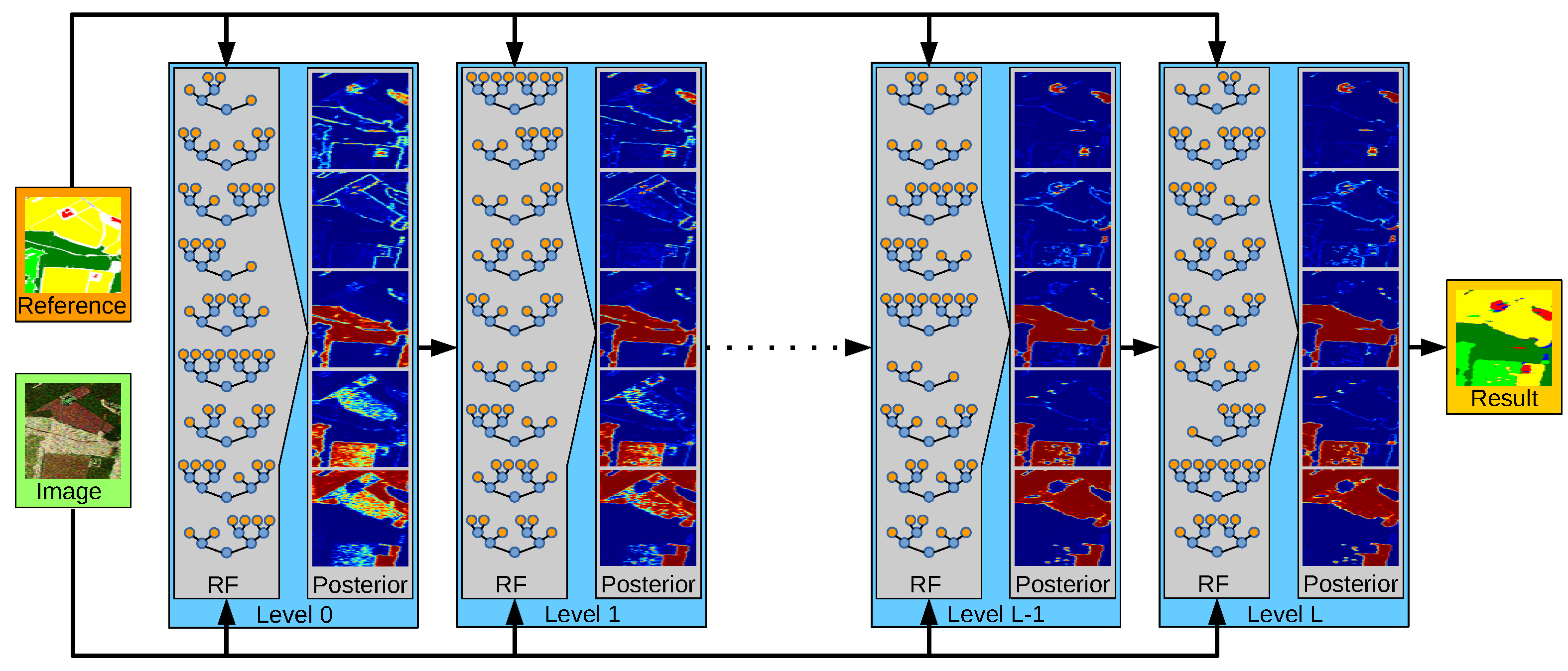
Two very different datasets are used to evaluate the proposed method. A color representation of the first dataset is shown in Figure 3a. It is a fully polarimetric image of pixels acquired over Oberpfaffenhofen, Germany by the E-SAR sensor (DLR, L-band) with a resolution of approximately 1.5 m. The area contains man made as well as natural structures. The annotation was acquired manually and consists of five different classes: City (red), Road (blue), Forest (dark green), Shrubland (light green), and Field (yellow) (see Figure 3b).
A dual-polarimetric image (i.e., and ) of pixels acquired over central Berlin, Germany, by TerraSAR-X (DLR, X-band, spotlight mode) with a resolution of approximately 1 m serves as a second dataset. Figure 6a shows the corresponding color representation. It shows a dense urban area but also contains a river and a large park area. It is manually labelled into six different categories, which are illustrated in Figure 6b, namely Building (red), Road (cyan), Railway (yellow), Forest (dark green), Lawn (light green), and Water (blue).
The following experiments are carried out on both datasets individually by dividing the image into five different parts. While the training data (20,000 pixels) are randomly sampled from four stripes, the fifth stripe is used for testing only and thus provides an unbiased estimate of the balanced accuracy, i.e., the average detection rate per class, which is well suited for imbalanced data sets and allows an easy interpretation of the results. The final balanced accuracy estimate is estimated as average over all folds. All quantitative as well as qualitative results in the following Section 4.2 are estimated on the test data of the individual folds.
4.2. Results
Figure 3c shows the label map composed by the individual test sets of all rounds obtained by the RF at level 0. This RF has only access to the image data itself and, of course, the labels of the training data during tree creation and training. It achieved a balanced accuracy of , which is already quite acceptable—a similar RF but based on a large set of real-valued pre-computed polarimetric features achieved [22]. However, the label fluctuates in some areas (e.g., within the central forest area) leading to noisy semantic maps, while other areas are consistently assigned with an incorrect label. Particular borders between different semantic classes are frequently misclassified. Figure 4 shows one of the problematic areas in greater detail (the corresponding image and reference data are shown in Figure 1). Apparently, the RF of this level associates edges within the image as being either city or road, leading to incorrect class assignments at the boundary between fields, forest, and shrubland (visible in the semantic maps within the first row of Figure 4). The second and third row of Figure 4 show the negative entropy and margin of the estimated class posterior and thus illustrate the degree of certainty of the classifier in its decision ranging from completely uncertain (margin equals zero, negative entropy equals −1, both shown in blue) to completely certain (margin equals one, negative entropy equals zero, both shown in dark red). The majority of the forest and field pixels show a high degree of certainty, while, in particular, the misclassified regions show a high degree of uncertainty. The remaining rows of Figure 4 illustrate the class posteriors for City, Street, Forest, Shrubland, and Field, respectively. The columns of Figure 4 show the progress of the learning through the individual levels of stacking. For space reasons, only levels 0, 1, 2, 5, and 9 are shown in ascending order in the corresponding columns. The largest changes occur within the first few levels. Using the semantic information provided by its predecessors as well as the original image data, each RF at a higher level is able to correct some of the remaining mistakes and to gain certainty in decisions already being correct. In particular, RFs of higher levels learnt that edges within the image only correspond to city or road if other criteria (e.g., certain context properties) are fulfilled as well. The large field area at the top of the image, which is confused with a big part as field in level 0 is now correctly classified as field. However, not all errors are corrected. An example is the large field area at the bottom of the image, which stays falsely classified as shrubland and the RFs gain even more certainty on this false decision. Nevertheless, overall, the classification improved significantly, which is also illustrated in Figure 3d, which shows the semantic map obtained by the RF of the last level and thus states the final output of the proposed method.
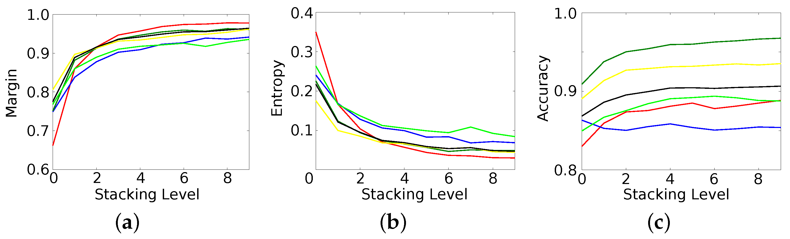
Figure 5 summarizes these results in a more quantitative manner by showing the progress of margin (Figure 5a), entropy (Figure 5b), and classification accuracy (Figure 5c) for the individual classes (same color coding as in the label maps above) as well as the average over all classes (in black). The classification accuracy does monotonically increase over all stacking levels starting at for level 0 and ending at at level 9. While there is a significant change in accuracy for the first levels, it starts to saturate quickly after roughly four levels. Interestingly, the different classes show quite different results. All classes benefit from stacking with streets as the single exception. The street class loses in accuracy, which drops from to at level 1 but stays then more or less constant. All other classes increase in accuracy but not to the same extent, while, for example, the accuracy of the field class appears to saturate already after level 2, with the forest class continuously slightly improving even at the last iteration.
Although the accuracy seems to quickly saturate, which means that the correct class obtained the maximal probability within the estimated posterior, the certainty of the RFs continuously improving as Figure 5a,b show. The changes, however, are larger at the first stacking levels and decrease significantly at higher levels. The reason why certainty saturates slower than accuracy is that accuracy only depends on the estimation of the correct class label. This requires that the correct label obtains a probability higher than the probability of all other labels. Once this happens, there won’t be any changes anymore. The certainty, however, can continue to increase until the winning label has consumed the complete probability mass of the distribution, i.e., has probability one while all other classes have probability zero.
Figure 6 shows the results of the proposed method on the second dataset. Despite the differences between both datasets (i.e., air- vs. spaceborne, fully polarimetric vs. dual-polarimetric, rural area vs. dense inner city area, etc.), the overall behaviour of the method is very similar in both cases. Classification accuracy (Figure 7c) increases monotonically for the different stacking levels. The RF at level 0 achieved an accuracy of (Figure 6c), while the semantic map of RF at the last level (Figure 6d) is correct. An RF based on real-valued, pre-computed features achieves only [22]. All classes benefit from stacking but again to a various degree. While river and railway, for example, could only gain and , respectively, forest and street improved by and , respectively. The largest changes occur at the first levels of stacking, while most classes only improve marginally with respect to accuracy after level 4. The certainty of the classifier (Figure 7a,b), however, continuously increases with more stacking levels. The final classification map contains significantly less label noise and shows smoother object boundaries.
5. Conclusions
This paper proposes using RFs within the stacking meta-learning framework for the classification of PolSAR data. It thus combines two ensemble learning strategies, i.e., the well established approach to average the output of several base learners (the individual trees within the RF) on the one hand, and, on the other hand, the lesser known but very successful method of stacking, i.e., including the estimates of the base learners as features for a subsequent model. The usage of the RF allows a seamless integration of both techniques: it not only provides a probabilistic estimate, i.e., the class posterior, which serves as optimal semantic feature, but also allows using this new feature without changing the overall framework simply by designed node tests that are defined over spatial-semantic probability distributions.
The performance on both datasets and for all classes are consistently improved over the different stacking levels, i.e., the results of each level are at least as good but mostly better than the results of the preceding level. The final results are more accurate by a significant margin, contain considerably less label noise, show smoother object boundaries, and have a higher degree of certainty of the classifier in its decision. Furthermore, the method itself converges, which makes a manual tuning of the number of stacking levels obsolete. The largest improvements happen within the first couple of levels, while performance saturates quickly (e.g., after four levels). This keeps the additional computational load at a limit and justifies the gain in performance.
It should be noted that this gain in accuracy comes basically for free, i.e., only at the cost of an increased training and prediction time—both increase (roughly) linear with the number of levels. However, neither more (e.g., more training samples) nor different (e.g., different sensors) data is needed. Furthermore, the same framework is used in all levels, i.e., the proposed method does not require several training and/or preprocessing procedures for different classifiers. Instead, no preprocessing and no explicit feature computation are performed, but the proposed stacked RF is directly applied to the local sample covariance matrices of the PolSAR data as well as to the probabilistic class estimates of previous levels.
Future work will focus on exploiting more information generated by the preceding RFs. The path a sample takes through each tree can serve as a powerful descriptor of local texture and thus complements to some extent the spectral and semantic properties used in this work. Furthermore, the estimated label maps provide not only local, but also more global context, which is currently ignored but can easily be included by node tests that sample large and more distant regions. Finally, the computational load of the stacking procedure can be decreased by more efficient node tests and by the fact that RFs in the first levels do not necessarily need to provide highly accurate estimations.
A second line of future work addresses the applicability of the proposed Stacked Random Forests to other types of remotely sensed data. This only requires an adaption of the applied node tests to the different data domains. In general, every image-based classification problem that can be solved by RFs sufficiently accurate should benefit from the proposed stacking framework.
Author Contributions
Olaf Hellwich contributed to the conception of the study, helped to perform the analysis with constructive discussions, and reviewed the manuscript. Ronny Hänsch contributed the central idea, implemented the methodology, performed the experimental validation, and wrote the manuscript.
Conflicts of Interest
The authors declare no conflict of interest.
References
- Tison, C.; Nicolas, J.M.; Tupin, F.; Maitre, H. A new statistical model for Markovian classification of urban areas in high-resolution SAR images. IEEE Trans. Geosci. Remote Sens. 2004, 42, 2046–2057. [Google Scholar] [CrossRef]
- Krylov, V.A.; Moser, G.; Serpico, S.B.; Zerubia, J. Supervised High-Resolution Dual-Polarization SAR Image Classification by Finite Mixtures and Copulas. IEEE J. Sel. Top. Signal Process. 2011, 5, 554–566. [Google Scholar] [CrossRef] [Green Version]
- Nicolas, J.M.; Tupin, F. Statistical models for SAR amplitude data: A unified vision through Mellin transform and Meijer functions. In Proceedings of the 2016 24th European Signal Processing Conference (EUSIPCO), Budapest, Hungary, 28 August–2 September 2016; pp. 518–522. [Google Scholar]
- Mantero, P.; Moser, G.; Serpico, S.B. Partially Supervised classification of remote sensing images through SVM-based probability density estimation. IEEE Trans. Geosci. Remote Sens. 2005, 43, 559–570. [Google Scholar] [CrossRef]
- Bruzzone, L.; Marconcini, M.; Wegmuller, U.; Wiesmann, A. An advanced system for the automatic classification of multitemporal SAR images. IEEE Trans. Geosci. Remote Sens. 2004, 42, 1321–1334. [Google Scholar] [CrossRef]
- Hänsch, R.; Hellwich, O. Random Forests for building detection in polarimetric SAR data. In Proceedings of the 2010 IEEE International Geoscience and Remote Sensing Symposium (IGARSS), Honolulu, HI, USA, 25–30 July 2010; pp. 460–463. [Google Scholar]
- Cloude, S.R.; Pottier, E. A review of target decomposition theorems in radar polarimetry. IEEE Trans. Geosci. Remote Sens. 1996, 34, 498–518. [Google Scholar] [CrossRef]
- He, C.; Li, S.; Liao, Z.; Liao, M. Texture Classification of PolSAR Data Based on Sparse Coding of Wavelet Polarization Textons. IEEE Trans. Geosci. Remote Sens. 2013, 51, 4576–4590. [Google Scholar] [CrossRef]
- Hänsch, R. Complex-Valued Multi-Layer Perceptrons—An Application to Polarimetric SAR Data. Photogramm. Eng. Remote Sens. 2010, 9, 1081–1088. [Google Scholar] [CrossRef]
- Moser, G.; Serpico, S.B. Kernel-based classification in complex-valued feature spaces for polarimetric SAR data. In Proceedings of the 2014 IEEE Geoscience and Remote Sensing Symposium (IGARSS), Quebec City, QC, Canada, 13–18 July 2014; pp. 1257–1260. [Google Scholar]
- Licciardi, G.; Avezzano, R.G.; Frate, F.D.; Schiavon, G.; Chanussot, J. A novel approach to polarimetric SAR data processing based on Nonlinear PCA. Pattern Recognit. 2014, 47, 1953–1967. [Google Scholar] [CrossRef]
- Tao, M.; Zhou, F.; Liu, Y.; Zhang, Z. Tensorial Independent Component Analysis-Based Feature Extraction for Polarimetric SAR Data Classification. IEEE Trans. Geosci. Remote Sens. 2015, 53, 2481–2495. [Google Scholar] [CrossRef]
- He, C.; Zhuo, T.; Ou, D.; Liu, M.; Liao, M. Nonlinear Compressed Sensing-Based LDA Topic Model for Polarimetric SAR Image Classification. IEEE J. Sel. Top. Appl. Earth Observ. Remote Sens. 2014, 7, 972–982. [Google Scholar] [CrossRef]
- Belgiu, M.; Dragut, L. Random Forest in remote sensing: A review of applications and future directions. J. Photogramm. Remote Sens. 2016, 114, 24–31. [Google Scholar] [CrossRef]
- Hänsch, R. Generic Object Categorization in PolSAR Images-and Beyond. Ph.D. Thesis, Technical University of Berlin, Berlin, Germany, 2014. [Google Scholar]
- Tokarczyk, P.; Wegner, J.D.; Walk, S.; Schindler, K. Features, Color Spaces, and Boosting: New Insights on Semantic Classification of Remote Sensing Images. IEEE Trans. Geosci. Remote Sens. 2015, 53, 280–295. [Google Scholar] [CrossRef]
- Zhou, Y.; Wang, H.; Xu, F.; Jin, Y.Q. Polarimetric SAR Image Classification Using Deep Convolutional Neural Networks. IEEE Geosci. Remote Sens. Lett. 2016, 13, 1935–1939. [Google Scholar] [CrossRef]
- Hänsch, R.; Hellwich, O. Complex-Valued Convolutional Neural Networks for Object Detection in PolSAR data. In Proceedings of the 8th European Conference on Synthetic Aperture Radar, Aachen, Germany, 7–10 June 2010; pp. 1–4. [Google Scholar]
- Zhang, Z.; Wang, H.; Xu, F.; Jin, Y.Q. Complex-Valued Convolutional Neural Network and Its Application in Polarimetric SAR Image Classification. IEEE Trans. Geosci. Remote Sens. 2017, PP, 1–12. [Google Scholar] [CrossRef]
- Criminisi, A.; Shotton, J. Decision Forests for Computer Vision and Medical Image Analysis; Springer: London, UK, 2013. [Google Scholar]
- Fröhlich, B.; Rodner, E.; Denzler, J. Semantic Segmentation with Millions of Features: Integrating Multiple Cues in a Combined Random Forest Approach. In Proceedings of the 11th Asian Conference on Computer Vision, Daejeon, Korea, 5–9 November 2012; pp. 218–231. [Google Scholar]
- Hänsch, R.; Hellwich, O. Skipping the real world: Classification of PolSAR images without explicit feature extraction. J. Photogramm. Remote Sens. 2017. [Google Scholar] [CrossRef]
- Wolpert, D.H. Stacked Generalization. Neural Netw. 1992, 5, 241–259. [Google Scholar] [CrossRef]
- Breiman, L. Stacked regressions. Mach. Learn. 1996, 24, 49–64. [Google Scholar] [CrossRef]
- van der Laan, M.J.; Polley, E.C.; Hubbard, A.E. Super Learner; U.C. Berkeley Division of Biostatistics Working Paper Series. Working Paper 222; U.C. Berkeley: Berkeley, CA, USA, 2007. [Google Scholar]
- Töscher, A.; Jahrer, M.; Bell, R.M. The BigChaos Solution to the Netflix Grand Prize. Netflix Prize Doc. 2009, 81, 1–10. [Google Scholar]
- Lee, J.S.; Pottier, E. Polarimetric Radar Imaging: From Basics to Applications; Taylor & Francis: London, UK, 2009. [Google Scholar]
- Goodman, N.R. Statistical analysis based on a certain multivariate complex Gaussian distribution (an introduction). Ann. Math. Stat. 1963, 34, 152–177. [Google Scholar] [CrossRef]
- Lee, J.S.; Grunes, M.R.; Kwok, R. Classification of multilook polarimetric SAR imagery based on complex Wishart distribution. Int. J. Remote Sens. 1994, 15, 229–231. [Google Scholar] [CrossRef]
- Anfinsen, S.N.; Jenssen, R.; Eltoft, T. Spectral clustering of polarimetric SAR data with Wishart-derived distance measures. In Proceedings of the 7th POLinSAR, Frascati, Italy, 22–26 January 2007. [Google Scholar]
- Conradsen, K.; Nielsen, A.A.; Schou, J.; Skriver, H. A test statistic in the complex Wishart distribution and its application to change detection in polarimetric SAR data. IEEE Trans. Geosci. Remote Sens. 2003, 41, 4–19. [Google Scholar] [CrossRef]
- Kersten, P.R.; Lee, J.S.; Ainsworth, T.L. Unsupervised classification of polarimetric synthetic aperture radar images using fuzzy clustering and EM clustering. IEEE Trans. Geosci. Remote Sens. 2005, 43, 519–527. [Google Scholar] [CrossRef]
- Barbaresco, F. Interactions between symmetric cone and information geometries: Bruhat-Tits and Siegel spaces models for high resolution autoregressive doppler imagery. Emerg. Trends Visual Comput. 2009, 124–163. [Google Scholar] [CrossRef]
- Arsigny, V.; Fillard, P.; Pennec, X.; Ayache, N. Log-Euclidean metrics for fast and simple calculus on diffusion tensors. Magn. Reson. Med. 2006, 56, 411–421. [Google Scholar] [CrossRef] [PubMed]
- Ho, T.K. The random subspace method for constructing decision forests. IEEE Trans. Pattern Anal. Mach. Intell. 1998, 20, 832–844. [Google Scholar]
- Breiman, L. Random Forests. Mach. Learn. 2001, 45, 5–32. [Google Scholar] [CrossRef]
- Breiman, L. Bagging predictors. Mach. Learn. 1996, 24, 123–140. [Google Scholar] [CrossRef]
- Hänsch, R.; Hellwich, O. Evaluation of tree creation methods within Random Forests for classification of PolSAR images. In Proceedings of the 2015 IEEE International Geoscience and Remote Sensing Symposium (IGARSS), Milan, Italy, 26–31 July 2015; pp. 361–364. [Google Scholar]
- Lepetit, V.; Fua, P. Keypoint Recognition Using Randomized Trees. IEEE Trans. Pattern Anal. Mach. Intell. 2006, 28, 1465–1479. [Google Scholar] [CrossRef] [PubMed]
Figure 1.
We propose stacking of Random Forests for the pixel-wise classification of PolSAR data, which gradually increases the correctness of the label map as well as the certainty of the classifier in its decisions. From left to right: detail of a PolSAR image; certainty of the RF illustrated as margin of the class posterior of the first (left side) and the last (right side) level; obtained classification maps at the first (left side) and the last (right side) level; reference data (colors denote different classes, see Figure 3b).
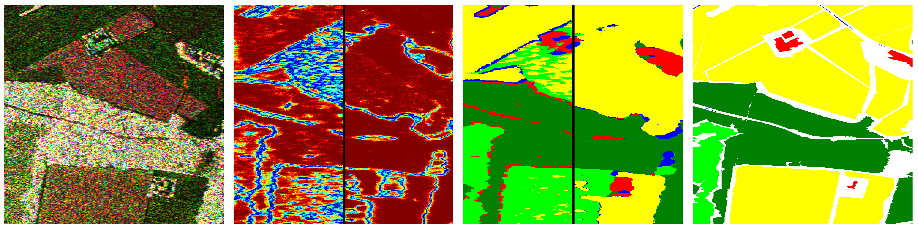
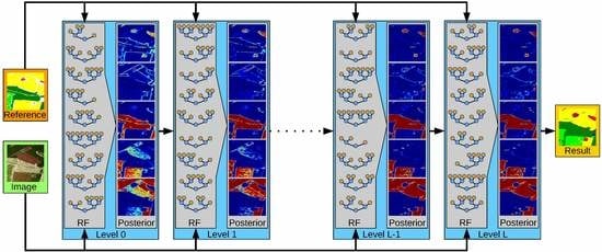
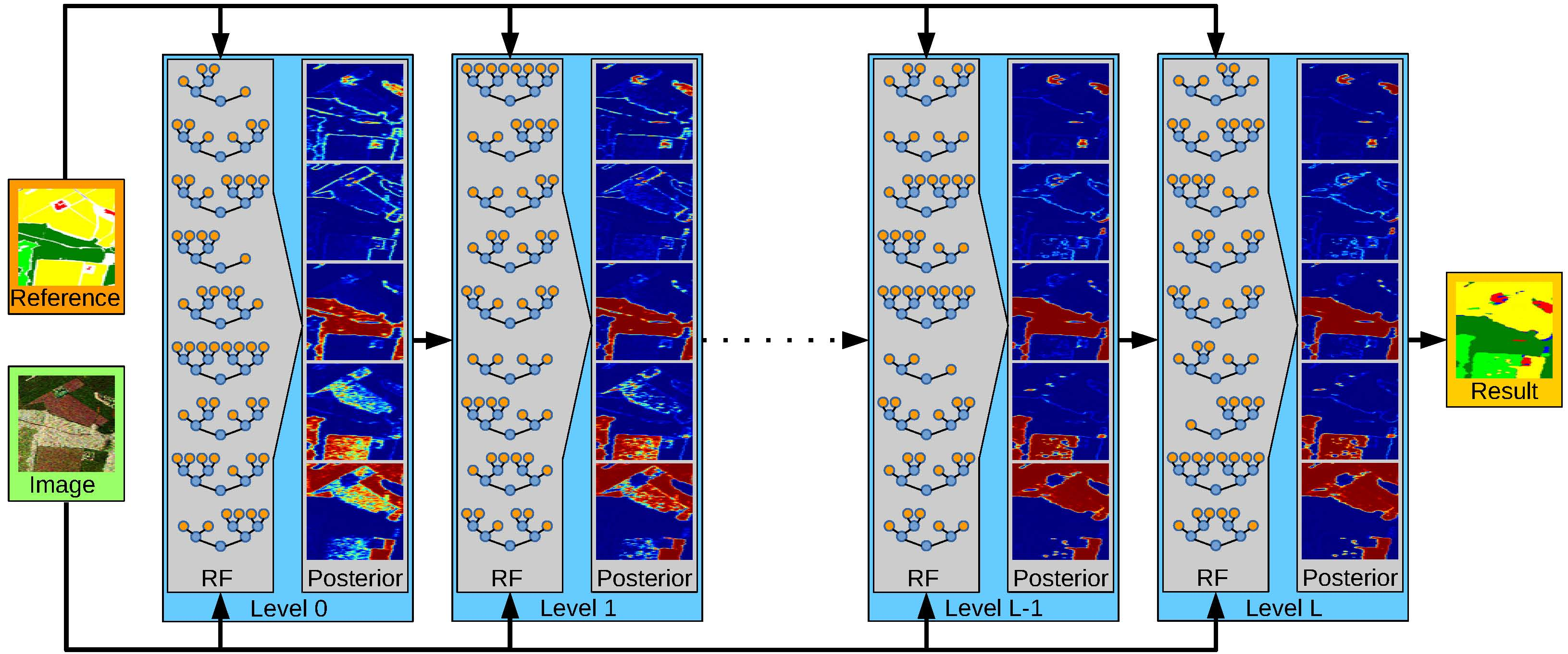
Figure 2.
The proposed stacking framework trains an RF at level 0 based on the image data and the reference data, while subsequent RFs use the estimated class posterior as additional feature. This allows a continuous refinement of the class decision and thus leads to more accurate semantic maps.
Figure 2.
The proposed stacking framework trains an RF at level 0 based on the image data and the reference data, while subsequent RFs use the estimated class posterior as additional feature. This allows a continuous refinement of the class decision and thus leads to more accurate semantic maps.

Figure 3.
Input data and results of the Oberpfaffenhofen dataset. (a) Image Data (E-SAR, DLR, L-Band); (b) Reference Data: City (red), Road (blue), Forest (dark green), Shrubland (light green), Field (yellow), unlabelled pixels in white; (c) Classification map obtained by the RF at Level 0; (d) Classification map obtained by the RF at Level 9.

Figure 4.
Detail of the Oberpfaffenhofen dataset (Image and reference data are shown in Figure 1). The columns illustrate levels 0, 1, 2, 5, and 9 of stacking. From top to bottom: label map (same color code as in Figure 3b); entropy; margin; class posterior of city, street, forest, shrubland, field.
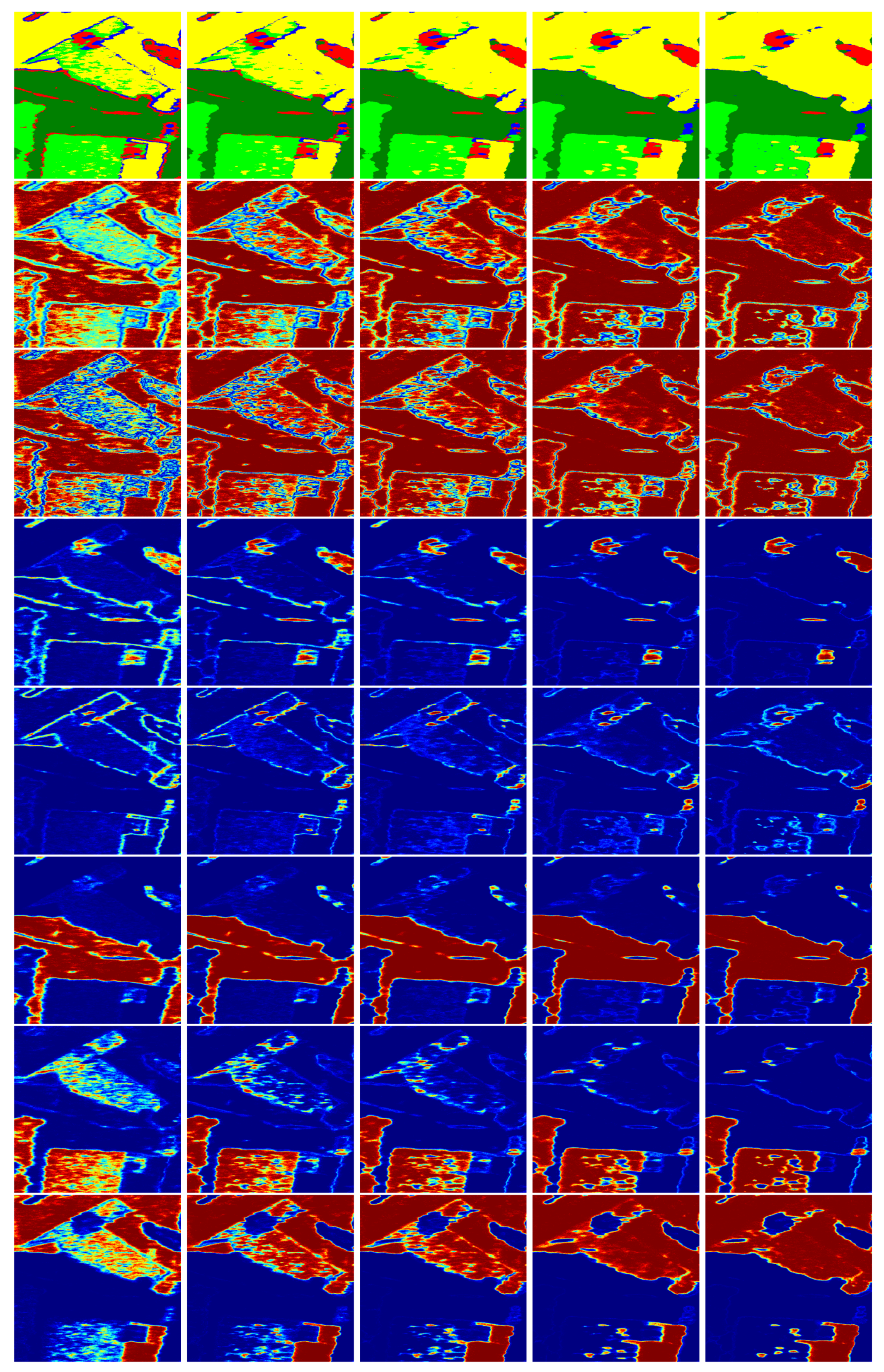
Figure 5.
Results over the different stacking levels on the Oberpfaffenhofen dataset. Colors denote different classes (see Figure 3b), black denotes the average over all classes. (a) Margin; (b) Entropy; (c) Accuracy.
Figure 5.
Results over the different stacking levels on the Oberpfaffenhofen dataset. Colors denote different classes (see Figure 3b), black denotes the average over all classes. (a) Margin; (b) Entropy; (c) Accuracy.

Figure 6.
Input data and results of the Berlin dataset. (a) Image Data (TerraSAR-X, DLR, X-Band); (b) Reference Data: Building (red), Road (cyan), Railway (yellow), Forest (dark green), Lawn (light green), Water (blue), unlabelled pixels in white; (c) Classification map obtained by the RF at Level 0; (d) Classification map obtained by the RF at Level 9.

Figure 7.
Results over the different stacking levels on the Berlin dataset. Colors denote different classes (see Figure 6b), black denotes the average over all classes. (a) Margin; (b) Entropy; (c) Accuracy.
Figure 7.
Results over the different stacking levels on the Berlin dataset. Colors denote different classes (see Figure 6b), black denotes the average over all classes. (a) Margin; (b) Entropy; (c) Accuracy.

© 2018 by the authors. Licensee MDPI, Basel, Switzerland. This article is an open access article distributed under the terms and conditions of the Creative Commons Attribution (CC BY) license (http://creativecommons.org/licenses/by/4.0/).
Share and Cite
MDPI and ACS Style
Hänsch, R.; Hellwich, O. Classification of PolSAR Images by Stacked Random Forests. ISPRS Int. J. Geo-Inf. 2018, 7, 74. https://doi.org/10.3390/ijgi7020074
AMA Style
Hänsch R, Hellwich O. Classification of PolSAR Images by Stacked Random Forests. ISPRS International Journal of Geo-Information. 2018; 7(2):74. https://doi.org/10.3390/ijgi7020074
Chicago/Turabian StyleHänsch, Ronny, and Olaf Hellwich. 2018. "Classification of PolSAR Images by Stacked Random Forests" ISPRS International Journal of Geo-Information 7, no. 2: 74. https://doi.org/10.3390/ijgi7020074
Note that from the first issue of 2016, this journal uses article numbers instead of page numbers. See further details here.