Modeling Spatial Interactions between Areas to Assess the Burglary Risk

Abstract

It is generally acknowledged that the urban environment presents different types of risk factors, but how the structural effects of areas influence the risk levels in neighboring areas has been less widely investigated. This research assesses the local effects of burglary contributory factors on burglary over small areas in a large metropolitan region. A comparative framework is developed for analyzing the effects of geographic dependence on burglary rates, and for assessing how such dependence conditions the community context and the urban land use. A local indicators spatial autocorrelation analysis assesses burglaries over five years (2011–2015) to identify risk clusters. Thereafter, effects of different variables (e.g., unemployment, building density) on burglary frequency are estimated in a series of regression models while controlling for changes in the risk levels of nearby surrounding areas. Results uncover strong evidence that the configuration of the surroundings influences risk. After controlling for area-based interaction, patterns are identified that contrast with the previous literature, such as lower burglary frequency in areas with higher tenancy in social housing units. Together the findings demonstrate that the spatial arrangement of areas is as crucial as contextual crime factors, particularly when assessing the risk for small areas.

1. Introduction

Crime analysts have commonly applied the ecological tradition to explain burglary concentrations in terms of socioeconomic and political structures [1]. The connection of unstable institutions and crime within areas is well established in the literature, but the extent to which crime is influenced by instability and crime problems of nearby surrounding areas has often been overlooked [2,3]. This omission detaches the crime analysis from practice because human mobility and interaction, and the decay of these with increasing distance, together induce changes to the distribution of risk factors [1]. In contrast, unilateral focus on risk within areas assumes that areas with uniform characteristics are equivalent and does not assess whether or not their neighbors are similar, akin to closing off crime scenes and assessing only the evidence found within each scene.

With exceptions, such as during the analysis of whole countries, or when assessing areas that have been sampled randomly with no respect to their geographic interconnectivity, mobility and interaction have significant implications to the measured observations [4]. One way to envision the fallacy of overlooking spatial interaction is through the hypothetical exchange of locations for two areas, one located in crime-prone zone, and the other on a crime-free zone. Since such a locational shift is bound to affect the resultant crime levels for both zones, it follows that interaction between areas can drive the overall crime statistics. Consistently, crime analysts often draw links from crime factors that stem from broader area-based processes, such as economic inflation, regional borrowing, and social stratification whose influences extend beyond areas [5]. However, few studies have investigated how localized criminogenic places coexist [5].

The necessity of investigating the nature and intensity of spatial relationships in this study is motivated, among other aspects, by the fact that routine activities cause formations of origin-crime paths that are spatially unconstrained. Transportation systems interconnecting small areas, cities and regions enable residents to leave their census delineated areas to work, shop, or visit friends each day [6], large numbers of people aggregate at different public places and/or for different events [7,8,9], and individuals are released from prisons to settle in geographically distributed areas [10]. Phenomena such as these often generate shifts in crime opportunities. Thus, while the structural compositions of areas are meaningful for explaining crime, the interaction occurring during routine activities is also highly relevant [11,12].

This crime investigation contributes knowledge about the implication of socio-structural effects for generation of burglary. More importantly, it also investigates risk effects that are due to spatial arrangement of areas. Burglary is convenient for this analytical design because previous studies have often focused on other volume crimes such as theft and violence [13,14,15]. Unlike with these crimes, offender–target investigation for burglary does not involve uncertainty of mobile targets. This allows a more focused analysis.

2. Area-Based Burglary Influences

Studies have applied theoretical frameworks for understanding crime, such as “collective efficacy” and “social disorganization” [13,16,17]. These theories attribute area-based risk clusters to two main causes: (a) variation in the ability of communities to exercise informal safety mechanisms; and (b) adverse aspects of areas that discourage individuals from intervening for the common good [15,17]. Therefore, vulnerable target environments allow offenders to establish a “comfort zone” that expands with increasing successes [18,19,20]. This results in clusters at specific areas [2,13,21,22], within specific household types and locations [23,24,25], and during specific times of the day or days of the week [21,26]. Environmental criminologists investigate such crime patterns by tracking offender journeys to crime [27,28]. However, offender-specific datasets are usually not detailed enough to provide all clues about offender interactions and how these lead to crime concentrations [28].

The increasing ability to conduct micro-level studies has led analysts to draw more information from attributes of the target areas as conditions for burglars’ choices. This line of investigation pursues the area-based socioeconomic and land-use factors which are likely to promote or hinder the development of crime [2]. Sociological studies have investigated links between burglary and concentrated disadvantage [22,25], high population density [29,30], disadvantage [1,20,25], and residential instability [31,32,33], and many significant associations have been found. In an extensive study of 352 U.S. cities over 30 years, Hipp [34] discovered that the level of economic stratification had significant implications for burglary. Cities which combined different economic levels in the same areas experienced higher risk levels that cities with uniform economies. However, cities with high socioeconomic stratification suffered high burglary rates irrespective of the economic configurations. Further evidence shows that the inability of residents to exercise informal social control can cause crime effects from the surrounding areas to be felt [13]. It was additionally discovered that the likelihood for victimization by burglary was higher in areas where affluent households bordered deprived households than in areas where affluent households were surrounded by surrounded by equally affluent households [35].

Structural aspects of the built environment have also been investigated. For instance, Ward and his colleagues [25] discovered that areas with high accessibility by the road network experienced a low burglary risk, while areas with higher affluence suffered higher rates despite good connectivity. The authors attributed this observation to the rational balance of risks and benefits by offenders. The prospect of increased profitability is likely to direct burglars to select a hunting area comprising affluent households than disadvantaged ones. It has also been proposed that certain urban land use features, such as commercial places and permeable roads (i.e., crime generators) attract large numbers of people for noble reasons, but nevertheless provide offending opportunities [2,8,10,19]. Many urban places also include crime attractors, such as drug markets, lending places, pawnbrokers, red-light districts that to lead to high crime concentrations because they host illegal activities and attract willing participants, with motivated offenders and vulnerable targets among these [8,10,36,37,38].

The discoveries above suggest that crimes result from both the risk factors available in areas and from nearby influences. Unfortunately, many of the studies highlighted above have assumed either that home–crime paths of burglars are randomly distributed or that no spatial constraint such as distance or connectivity of areas is present [2]. Little work has been done to discover whether interconnectivity generates more crime opportunities in certain places than others [2,10,38]. Because crime influences transect the boundaries of census tracts, reliable risk estimation must take into account the interaction that occurs among groups of areas. The analysis of this paper provides one of the early investigations into area-based interactions and patterns of officially reported burglaries by exploring two questions:

• To what extent does the spatial arrangement of areas mediate the structural influence on an area’s internal burglary risk?
• How do risk factors of interconnected areas affect the cumulative burglary frequency?

The rest of this paper is structured as follows. First we present the study area and methods. Results are presented thereafter, as well as a discussion of the implications. The paper concludes with policy recommendations.

3. Materials and Methods

3.1. Study Area

The focus of this study is the metropolitan region of Greater London, the largest urban area of the UK and the most populous in the European Union [39]. This area was chosen for three main reasons. First, the London region is a busy commercial environment with different types of crime generators, rising house prices, and accelerating rates of crime [40,41,42]. It therefore offers an ideal scene for investigating area-based crime influences. Secondly, high socio-economic inequality characterizes the London region. The gap between the London rich and poor is one of the largest in Europe, with Inner London being the most economically unequal region of England [40]. On the one hand, certain areas on the east, north and north-west of London were classified by the UK indices of multiple deprivation as the most deprived in all of England [43]. On the other hand, the collective value of properties in ten boroughs in London’s downtown outstrips the combined value of properties in Wales, Northern Ireland, and Scotland [44]. Such pronounced economic inequality is bound to affect crime levels. Finally, the London authorities have made different types of highly detailed datasets freely available for research, a factor that is bound to promote future comparative investigations of this kind.

3.2. Data and Variables

The study data were obtained from various sources. The dependent variable is continuous and denotes the number of burglaries per hectare. It makes use of 425,393 police-recorded burglary events that occurred throughout the Greater London, UK region over five years (2011–2015).

The analysis employs 12 independent variables. A number of socioeconomic indicators were drawn from the ONS census data for 2011 as guided by the previous literature [1,12,35,36,45]. The first four variables correspond to conditions of areas where social problems are likely to arise and affect informal controls over crime [14,17]. Different proportions of households were measured with respect to; (1) unemployment (UNEMP); (2) no automobile (NOAUTO); (3) no central heating (NOHEAT); and (4) living on social housing units (SOCHSE). Three additional variables control for factors that can directly aggravate the burglary behavior, consistent with previous studies [15,17,35]; (5) the value of mortgage lending for post code sectors (MORTAGE) was obtained from the ONS and averaged over the four quarters of 2014. We employed area-weighted means to extract values for the analysis units. Values correspond to the proportions of data in originating areas that intersect target areas, assuming a uniform distribution of values within areas. For example, if the originating area has a mortgage lending value of 5 million £ and it constitutes a half of the target area, it contributes 2.5 million as the area-weighted mean value to the target area. (6) House prices (HSEPRICE) were obtained from the ONS at the geography of analysis areas; and (7) the presence of payday lending shops, mortgage brokers, and pawnbrokers (LENDERS) was determined using actual locations of these facilities. LENDERS quantifies the potential for criminogenesis because such facilities create adequate grounds for burglary [46,47,48]. The variable, LENDERS was constructed by searching the yellow pages and querying unique locations of operational facilities using the Google mapping application. A weighted exposure was measured over the road network and employed the official roads data of the Ordnance Survey. This applies inverse distance weights using the shortest path route by road from an area’s population-weighted centroid to the location of facilities. The weights employs the difference between the pre-defined threshold distance value (1 km) and the distance value of each facility to an area’s centroid over the maximum value, summed for all observations within 1 km.

Two variables correspond to affluent areas and crime mitigating influence, employing the ONS census data for the analysis areas; (8) INCOME is the total median household income per year, averaged over five years (2008–2013); and (9) HOMEOWN represents the proportion of residential properties that are owned outright. Finally, three variables signal opportunities for offender–target interaction [1,17,30,48,49]; (10) POPDENS is a variable measuring population density, i.e., the number of persons per 100 m²; (11) DIST2CITY represents proximity to the City of London. It employs inverse distance weights using the shortest path from each area’s centroid to the City. This measure was adjusted for the decreasing distance of areas to the city center. It represents the difference between the maximum recorded distance and the area’s distance, weighted by the maximum distance value, i.e., 1 − [(d_max − d_ij)/d_max]); (12) BUILDDENS is the number of buildings per hectare and employs the Ordnance Survey’s latest official release of building footprints (July, 2015).

3.3. Methods

This study is focused on examining effects of burglary between small interlinked areas. Spatial interaction was hence conceptualized as a measure of contiguity for observation areas (n = 4,835). While differences between various contiguity-based weighting schemes were not substantial, the binary-weighted measure (0 = not neighbor, 1= neighbor) was found to be effective for avoiding artificial clustering, as consistent with previous observations [6,50,51,52]. First, local burglary clusters were investigated against different types of burglary-influencing factors using bivariate local indicators of spatial autocorrelation (LISA; [51]). Bivariate LISA assesses local correlations involving the cross-product of standardized values for one variable (e.g., burglary rates) and those of averaged neighboring values of another variable (e.g., unemployment rates) [53]. The statistic reports significant clusters (p < 0.05) of four types: high-high (areas of high clusters surrounded by areas of high clusters), low-low (areas of low clusters surrounded by areas of low clusters), high-low (areas of high clusters surrounded by areas of low clusters) and low-high (areas of low clusters surrounded by areas of high clusters) [51,52].

Additionally, four regression models were estimated for the burglary data; an ordinary least squares (OLS) model and three spatial models (i.e., spatial lag model—SLM, spatial error model—SEM, and spatial Durbin model—SDM). The latter three models controlled for distinct aspects of spatial interaction. On the one hand, based on the hypothesis that risk probabilities in an area are influenced by risk probabilities in its nearby surrounding areas [54], the SLM adopted the following nonlinear adjustment to ordinary least-squares estimation:

$$ln(y)=\mathsf{\rho }Wln(y)+{\displaystyle \sum _{i=1}^{12}{X}_i{\mathsf{\beta }}_i+\mathsf{\epsilon },\mathsf{\epsilon }~N(0,{\mathsf{\sigma }}^{2}I),}$$

(1)

where y is the natural log of burglary rates (i.e., events per ha.) and X is a 12 by n design matrix of the 12 predictor variables listed in

Table 1. Description of predictor variables for the regression models of burglary (n = 4,835).

	Variable Description 1	Alias 2	Min.	Mean	Max.	S.D.
1.	Unemployment	UNEMP	0.008	0.082	0.297	0.046
2.	No automobile in household	NOAUTO	0.027	0.400	0.863	0.185
3.	No heating system	NOHEAT	0.000	0.027	0.135	0.016
4.	On social housing	SOCHSE	0.000	0.235	0.909	0.202
5.	Mortgage lending (£)	MORTGAGE	2,790,728	241,021,712	687,895,559	104,665,763
6.	House price (£)	HSEPRICE	93,000	335,119	2,910,350	214,504
7.	Payday lenders (inverse dist.)	LENDERS	0.000	0.084	2.968	0.267
8.	Average household income (£)	INCOME	23,062	36,698	79,404	6,819
9.	Homeownership	HOMEOWN	0.032	0.511	0.974	0.220
10.	Population density (persons per 100 m.)	POPDENS	0.012	0.959	6.824	0.612
11.	Distance to the City	DIST2CITY	0.000	0.598	1.000	0.208
12.	Building density (buildings per ha.)	BUILDDENS	0.290	5.426	15.823	2.304

Notes: ¹ Regression models employ standardized predictor variables; ² Variable names are represented by aliases in the subsequent reference.

. The parameters β_i, ε, σ², and I correspond respectively to the regression coefficients, the vector of residuals, residual variance, and the identity matrix (i.e., the n × n diagonal matrix of 1s). ρ quantifies the spatial autocorrelation using an n × n spatial matrix of binary contiguity-based weights, W.

The SDM extends the SLM to include effects of burglary-contributory factors in the surrounding area [55]. Hence, the SDM has an additional parameter of the auto-regressive process for each spatially lagged predictor and takes the following form:

$$ln(y)=\mathsf{\rho }\mathit{W}ln(y)+{\displaystyle \sum _{i=1}^{12}{X}_i{\mathsf{\beta }}_i+WX\gamma +\mathsf{\epsilon },\mathsf{\epsilon }~N(0,{\mathsf{\sigma }}^2\mathit{I}),}$$

(2)

where γ is a (12 × 1) parameter measuring the marginal impact of variation in nearby areas on burglary. Estimation of the two spatial models, SLM and SDM takes into account spill-over effects, unless observations are randomly distributed in space (i.e., ρ = 0). These correspond to three types of equilibrium effects modeled using Bayesian Markov’s Chain Monte Carlo (MCMC) simulation approach [50]; (1) direct impact measures effects of contextual variables on the burglary risk in the immediate location, as well as effects of feedback that cascades through the surrounding areas and returns to the area where the adjustment process was initiated; (2) indirect impacts denote effects of contextual variables in the immediate area on the burglary risk of all its neighbors; (3) total impacts is the sum of direct and indirect impacts [54].

The final spatial model, the SEM, is estimated under the hypothesis that burglary variation is induced by unknown or omitted factors. It hence models the spatial autocorrelation of residuals:

$$ln(y)={\displaystyle \sum _{i=1}^{12}{X}_i{\mathsf{\beta }}_i+\mathsf{\upsilon },\mathsf{\upsilon }=\lambda W\mu +\mathsf{\epsilon },\mathsf{\epsilon }~N(0,{\mathsf{\sigma }}^{2}I),}$$

(3)

where υ is a spatially correlated error term and λ is the coefficient of spatial dependence. The SEM does not model equilibrium effects. This is because the matrix elements which link the spatial effects parameter, λ with the regression coefficients, β are usually zero [54].

Tests for the clustering of model residuals employed the Moran’s I coefficient and standard deviation. Goodness of fit tests assessed the Akaike Information Criteria (AIC) and R² values of competing models. Additionally, likelihood ratio statistics tested the benefit of modeling spatial effects over applying a non-spatial linear regression to the burglary data.

4. Results

This section presents the identified burglary risk measurement in terms of crime concentration patterns, spatial clusters and correlations.

4.1. Exploratory Analysis

Areas experienced an average of 4.694 burglaries per hectare and significant variation in the burglary rates (min. = 0, max. = 35.986, S.D. = 3.529). The highest burglary rate, 36 crimes per hectare, was recorded for an area located near the City of London. In contrast, two areas located further away from the City registered no burglary over five years. Observing these areas, one notices that aspects of the nearby surrounding had significant influence on risk (Figure 1). The most burglary prone area (labeled “i”) has two distinctive features. First, its neighbors also suffered high victimization. Secondly, it has a high building density, and buildings in the surrounding areas are also clustered. The burglary-free areas, labelled “j” and “k” in Figure 1 are both surrounded by areas that also experienced few burglaries. It seemed that the strategic location of area k near docking facilities and the river Thames protected it from the burglary influence emanating from areas on the eastern side. Because of this extraneous influence, the comparison of safe versus risky places proceeds with reference to the areas, i and j.

The two areas i and j have several distinct features both in terms of their own characteristics and the configurations of their neighbors (Figure 2). The latter is more affluent, with higher levels of household income, homeownership, and house prices, and it is surrounded by areas that are less affluent than itself. In contrast, the neighbors of area j are clearly more affluent (Figure 2D,H, and J), and this may have reduced the attraction of this area for burglary. Both areas, i and j are comparable in their mortgage status and the absence of payday lenders, but area i has a significantly higher exposure to payday lending emergent from its neighbors on the north-west. Finally, i is more densely populated than j, and it is also surrounded by densely populated areas. Cumulatively, these characteristics may have caused the area, i to become a more likely target for burglary than the corresponding area, j.

Table 1 presents the descriptive statistics for predictor variables. Mortgage lending had the highest mean value and the lack of central heating was the least valued. Exposure to payday lending and pawnbroker facilities was the most varied across areas, with a larger value for the standard deviation (i.e., 0.267) than for the mean (i.e., 0.084) of the variable, LENDERS. Variation was also tremendous for the proportion of households on social housing (mean = 0.235, S.D. = 0.202), and the population density (mean = 0.959, S.D. = 0.612). Overall, all the predictor variables registered a significant amount of variation, partly because of heterogeneity of the metropolitan region and also due to the large number of observation areas. This led to the question of whether such variation would impact the variation in burglary concentrations. The disparity in values across variables also called for scaling of the predictor variables prior to regression analyses to make the coefficients estimates more legible.

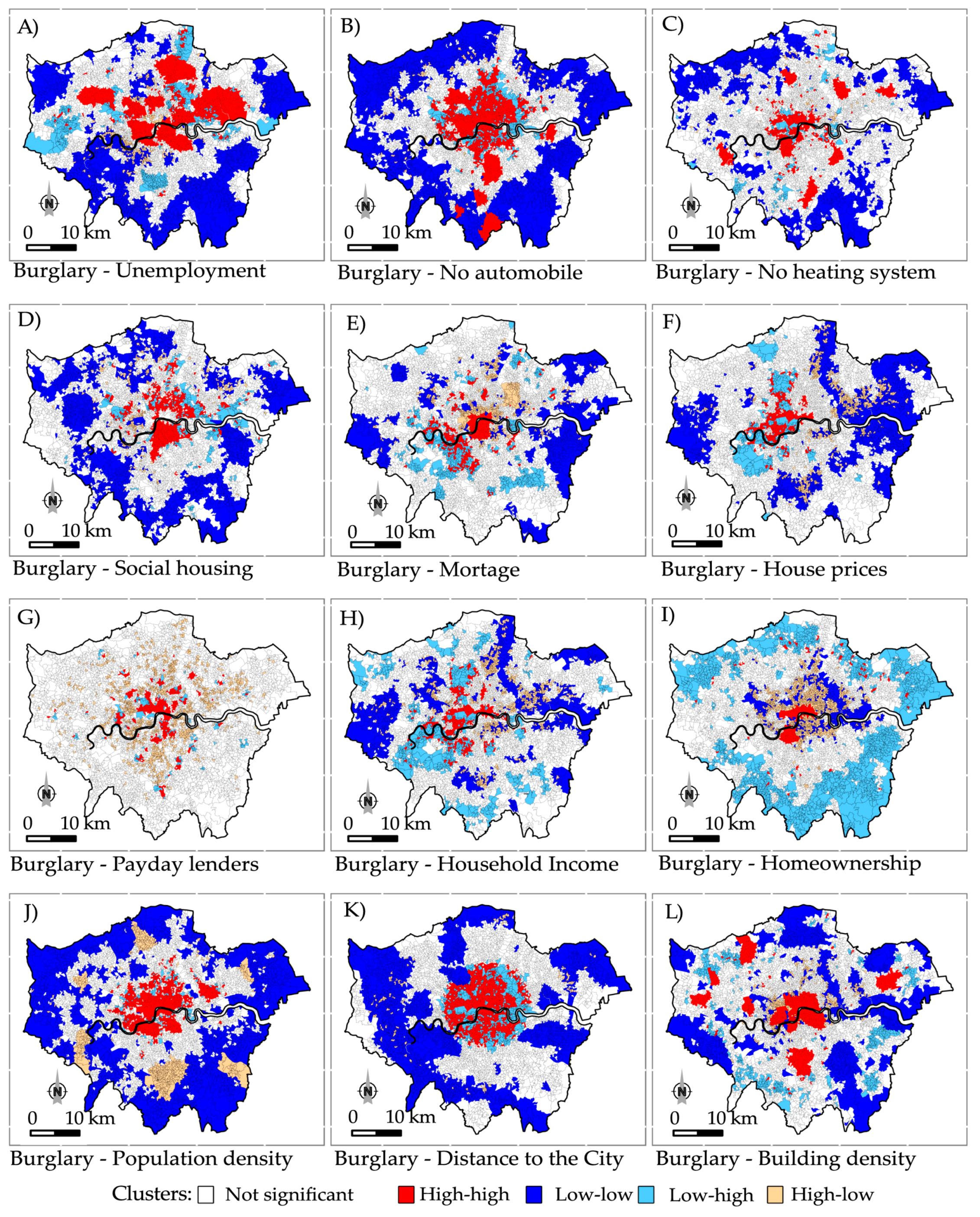
4.2. Detecting Spatial Clusters

A global assessment identified substantial clustering of burglary rates over geographic space (Moran’s I = 0.593, z-score ~ 70.195). At the local level, dense and statistically significant risk clusters were discovered for all predictor variables at the p = 0.05 level after 99,999 randomization tests (Figure 3). Particularly, the center of the study region including the City of London had clusters of high burglary risk surrounding high values of risk factors, consistent with the previous observation in (Figure 2 A,C,G, and K). The densest high-high clusters were detected for unemployment, households without motor vehicles, population density, and distance to the City. Specifically, the latter variable had the increase in its values being directly proportional to risk (Figure 3K). Pockets of high risk were densely clustered from the City, and they spread outwards in a circular manner to several the nearby areas. Afterwards there were low-high clusters in intermediate areas and low-low clusters near the periphery. Similarly, the presence of payday lenders had an outward influence from the City on risk in areas nearby (Figure 3G). The central region had high-high clusters spreading out into pockets of high burglary-low lending facilities in all directions.

The region’s periphery had either clusters of no significance or low-low clusters for many variables. In line with the expectation, homeownership influenced a risk reduction overall, and particularly in peripheral areas where dense low-high risk clusters could be found. However, two dominant types of risk clusters were associated with homeownership near the central region; high-high, in which risk existed in surrounding areas despite increased homeownership and high-low, where burglary was frequent near areas with low homeownership. The former observation coincides with the previous observation of high burglary risk in an area bordered by areas with large numbers of homeowners (Figure 2G)

Unlike many variables which registered high-high clusters around the City itself, high unemployment and social housing had no significant clustering with the burglary in this area. A possible explanation is that effects of these two variables were mediated by the high numbers of workers in the City, and the largely commercial land use respectively. Nevertheless high-high clusters of risk and unemployment were the densest and most widespread overall and especially in the northern areas. This is consistent with the hypothesis that burglars can comprise employed persons who discover opportunities in the course of daily interaction [12]. Other elements of the city’s structural profile appear to have registered as burglary generators. For example, dense clusters could be found in London’s downtown where high burglary rates occurred near densely populated areas and near areas with high building density.

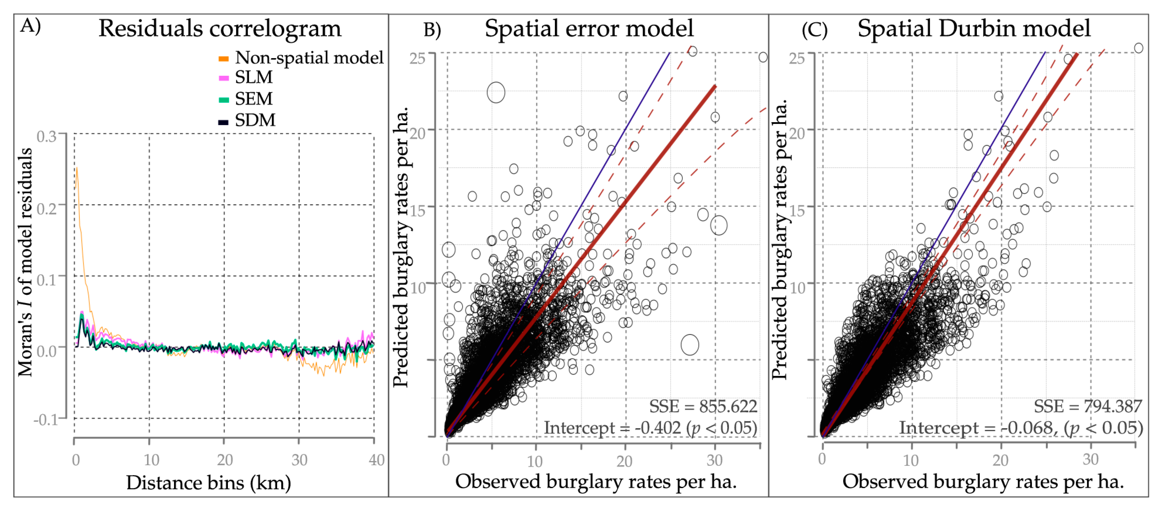
4.3. Regression Analysis

Lagrange multiplier diagnostics of regression models estimated positive and significant Moran’s I values for the spatially-lagged burglary variables and residuals.

Table 2. Parameter estimates of non-spatial and spatial models of burglary in Greater London output areas (n = 4,835).

Parameters	Non-spatial Model	Spatial Lag Model	Spatial Error Model	Spatial Durbin Model
Adjusted R2	0.652	0.690	0.695	0.742
AIC	6,087.519	5,543.231	5,448.203	5,065.682
Schwarz criterion	6,178.291	5,640.484	5,545.458	5,241.326
Rho (ρ)	-	0.383 ***	-	0.468 ***
Lambda (λ)	-	-	0.450 *	-
Log likelihood (d.f) 3	−3,030 (14)	−2,757 (15)	−2,709 (15)	−2,506 (27) 4
Likelihood ratio	-	546.293 ***	631.320 ***	644.741 ***
Residual variance (σ2)	0.217 *	0.178	0.171	0.165
Residuals Moran’s I	0.245 ***	0.036 **	0.021 *	0.013
Moran’s I z-score	29.032	4.301	2.945	1.095

Notes: Significance: “*” p < 0.05; “**” p < 0.01; “***” p < 0.001; ³ Likelihood ratio tests estimate the model improvement after modeling spatial dependence; ⁴ The spatial mixed model has additional parameters equal to the number of predictor variables.

shows the model diagnostics for the ordinary least squares (OLS) model and the three spatial models; the spatial lag model (SLM), the spatial error model (SEM), and spatial Durbin model (SDM). Coefficients of spatial autocorrelation were significant for all the spatial models. Specifically, high rho values were estimated for the lag models, the SLM and SDM (ρ = 0.383 and ρ = 0.468, p < 0.001), and the spatial error term was also moderately significant (λ = 0.450, p < 0.05). This observation highlighted the implications of modeling spatial effects. The SDM had the highest log-likelihood estimate (−2.506), despite this model having twelve degrees of freedom more than the SLM and SEM. Likewise, the Akaike information criterion (AIC) and Schwarz criterion (SC) estimates all showed that the SDM was substantially the most reliable risk model. The coefficient of model determination (R²) was also the highest for the SDM, and it appears that accounting for spatial dependence in both burglary and the contextual factors caused a significant increase in the model estimation reliability.

Spatial models had less clustered residuals than the OLS regression model which registered a highly significant Moran’s I value (i.e., 0.245, z-score = 29.032, p < 0.001). However, the Moran’s I estimate was also moderately significant for the SLM (z-score = 4.301, p < 0.01), suggesting that the adjustment for spatial autocorrelation in the dependent variable alone was insufficient. Of the two best models (SEM and SDM), the latter had the least spatially autocorrelated residuals. Figure 4 examines the residuals for all models over geographic space. It emerges from observing the residuals pattern that all the four models had clustered residuals within a distance of 4 km (Figure 4A), but the OLS regression residuals were the most clustered at this distance. Thereafter, OLS residuals exhibited a negative spatial autocorrelation beyond 30 km. Consistent with the previous observation (Table 2), residuals for the SEM and SDM were the least correlated.

Examining burglary rates plotted against the back-transformed regression values predicted by the SEM and the SDM—the two best performing models—uncovered a distinct and positive correlation for the latter (Figure 4C). The SEM had several outliers affecting its prediction power. Additionally, residual variance was 7% lower for the SDM (SSE ≈ 856) than the SEM (SSE ≈ 904). These observations and the goodness-of-fit statistics (Table 2) guided the subsequent analysis to adopt the SDM.

Table 3. Estimates from the spatial Durbin model of burglary rates and the nearby impacts (n = 4,835).

Variable	Burglary Estimate			Direct Impact 5			Indirect Impact			Total Impact
	Estimate	S.E	z-value	Estimate	S.E	z-value	Estimate	S.E	z-value	Estimate	S.E	z-value
Intercept	−0.068 *	0.028	−2.441	-	-	-	-	-	-	-	-	-
UNEMP	0.724 *	0.372	1.944	0.030 *	0.008	3.403	0.017 *	0.008	2.153	0.047*	0.025	1.910
NOAUTO	1.220 ***	0.163	7.498	1.042	0.861	1.210	0.598	0.385	1.555	1.640	1.603	1.023
NOHEAT	2.170 **	0.485	4.472	2.395 ***	0.392	6.111	1.375 *	0.718	1.914	3.769	2.476	1.522
SOCHSE	−0.673 ***	0.097	−6.964	−0.914 *	0.396	−2.309	−0.524	0.436	−1.203	−1.438	0.764	−1.883
MORTGAGE	0.012	0.017	0.887	0.014	0.106	0.132	0.008	0.005	1.667	0.023	0.018	1.282
HSEPRICE	0.015	0.014	1.071	0.041 *	0.021	1.924	0.023 *	0.008	3.012	0.064 *	0.029	2.227
LENDERS	0.041 *	0.010	4.230	0.023 **	0.003	6.324	0.013 ***	0.002	6.573	0.036 *	0.011	3.192
INCOME	−0.023	0.029	−0.792	−0.047	0.032	−1.447	−0.027	0.022	−1.208	−0.074	0.069	−1.066
HOMEOWN	−0.450 *	0.132	−3.418	−0.632	0.347	−1.820	−0.363 *	0.136	−2.677	−0.995	0.552	−1.804
POPDENS	0.336 ***	0.016	20.624	0.321 *	0.121	2.655	0.184	0.100	1.840	0.505 *	0.250	2.020
DIST2CITY	7.647 ***	0.942	8.121	0.348 **	0.085	4.108	0.200 *	0.054	3.701	0.547 *	0.156	3.512
BUILDDENS	0.106 ***	0.035	9.602	0.100	0.055	1.823	0.057 *	0.029	1.969	0.157	0.086	1.836

Notes: Significance: “*” p < 0.05; “**” p < 0.01; “***” p < 0.001. Significant values are displayed in bold; ⁵ Standard errors and significance values of direct, indirect and total impacts are estimated after 99,999 randomization tests.

presents burglary estimates of the SDM regression model. Direct, indirect, and total (direct + indirect) effects of the regression estimates were measured between order 0 (the immediate area) and order 3 (the third nearest neighbor). All risk effects were statistically significant except for three variables; MORTGAGE, HSEPRICE, and INCOME. Additionally, more than half of the direct and indirect impacts were significant, implying that interaction of nearby areas had a profound influence on risk. For example, the direct effect for the variable, NOHEAT (i.e., 2.395) was substantially higher than the partial effects estimated for this variable (i.e., 2.17). This implies that areas experienced a burglary increase of 0.225 due to unemployment in the areas nearby. However, indirect effects were less strongly felt. Contextual factors affected a lower magnitude of cumulative risk in the surrounding areas, possibly owing to distance decay. Similarly, the overall feedback effects (the sum of direct and indirect impacts) were less significant than the actual burglary estimates in areas for many variables.

All socioeconomic indicators of disadvantage except SOCHSE (i.e., UNEMP, NOAUTO, NOHEAT and POPDENS) were significantly correlated with high risk. The magnitude of risk influence was also much higher for these variables than for most contextual factors. However, DIST2CITY had the greatest coefficient value overall (β_DIST2CITY = 7.647, p > 0.001). Additionally, this variable and two others (UNEMP, LENDERS) had significant values for all risk measurements, including the spill-over effects. The coefficient of HSEPRICE was not significant, but both its direct and indirect influences were significant. While from the observation of Figure 2G,H, it seemed that household income would be correlated with risk, the SDM estimated no significant influence for the variable INCOME for either the coefficient or spillovers. Similarly, the variable, MORTGAGE was not significantly correlated with burglary, and this agrees with the uniform values observed earlier for areas of low versus high risk (Figure 2A,B).

HOMEOWN had a negative influence on risk, and increased homeownership in surrounding areas had negative influence on the immediate area (indirect impact = −0.363, p < 0.05). This observation is consistent with the risk profile observed for safe areas (Figure 2J) and with the dense low-high clusters that were found for burglary-homeownership, particularly in the peripheral areas (Figure 3I). Nevertheless, the influence of homeownership on risk reduction in nearby areas was moderate, and its direct and total impacts were generally insignificant.

Unexpectedly based on previous studies [5,15], the coefficient estimate was negative for the variable SOCHSE, and the direct impact for this variable was also negative and significant (p < 0.05). The variables DISTANCE and BUILDDENS were highly significant to increased risk, and the feedback effects were also relatively high for these variables.

5. Discussion

This study has addressed the underexplored phenomenon of spatial interaction between the small areas of an urban metropolis, and how this interaction affects burglary concentrations. The research has examined effects of disadvantage (e.g., unemployment, absence of central heating systems, social housing) and affluence (e.g., homeownership, house price) in the area-based burglary risk, while also controlling for effects of these factors on burglary rates in the nearby surrounding areas. Prior research has generally focused on the relationship between burglary and contributory effects within areas, and the spread of burglary opportunities to nearby surrounding areas has been overlooked. Additionally, this burglary investigation has considered both the socioeconomic configuration of community context and the place-based structural aspects of the urban land use (e.g., the exposure to payday lenders, building density). In these respects, the results from this systematic modeling contributes new evidence for law enforcement practitioners and policymakers.

Initially, investigation of local spatial clusters was conducted to determine whether risk aspects in an area had implications on the neighboring risk. Dense and widespread clusters were discovered for all variables, confirming this hypothesis. The analysis also compared different regression models of burglary, both spatial and non-spatial, and discovered that the most accurate risk model included spatial dependence of both the burglary rates and the contributory factors. This is an important insight for analysts seeking to model risk using geographically referenced observations across small areas.

Focusing on the target area attributes, four out of the five measures of area-based disadvantage examined were significantly related with increased probability for burglary. Areas with high unemployment, high population density, and/or which lacked a motor-vehicle and central heating system had higher likelihood for burglary. This is consistent with previous studies that attributed high burglary risk with populous areas [29,30] and high vulnerability of households with insufficient controls [13,17,45]. It also agrees with the hypothesis related to increased risk within unstable institutions [16,17]. Nevertheless, strong evidence was also found for low burglary risk being experienced in areas with a large number of social housing units, and this did not confirm the above hypothesis or past observations that have linked burglary with housing-related disadvantage [5,15]. Instead, the observation suggests a certain capability of communities to exercise collective efficacy against burglary in spite of disadvantage. As such, the results here can inform policies that seek to promote and develop risk mitigating factors in underprivileged areas. An alternative explanation for the reduced risk among households under the social scheme is spatial, and relates to the reduced attraction for burglars in these areas. Burglars are expected to look for profitable targets, and it is unlikely that they will hunt for opportunities among houses that have clearly perceived disadvantage. It was discovered in a previous study that deprived but close-knit areas of Florida, USA suffered a low level of burglary risk [25]. This is also consistent with observations from (Figure 2D,H,J). The area that suffered the lowest risk was one with reduced opportunity, since it is well known that burglars often seek targets in affluent areas [30,35]. Additionally, the clear-cut estimate for social housing stems from the structural configuration of this indicator. Unlike with certain broader census-based measures, such as unemployment, clusters of place-based factors, such as social housing schemes are usually more prominently outlined within and between areas. An underexplored possibility has therefore been the extant spatial interaction among the close-knit communities that have a mutual disadvantage.

Burglary rates were significantly lower in areas with high homeownership, in line with other past findings [21,32,35,36]. This pattern supports the “collective efficacy” hypothesis relating affluent and stable communities with increased control over crime. However, after controlling for the influence of neighboring areas, the most crime-prone area was found in a relatively affluent area with high homeownership. Additionally, areas with high homeownership did not significantly mitigate the burglary risk in the nearby surrounding. This signified the capability of nearby influences to reduce the mitigating effect of homeownership on risk.

With respect to the structural influence of the urban land use, the likelihood for burglary increased with the increase in distance to the City, while clusters of low burglary probability were more prominent in peripheral areas. This observation has several key implications. The first is the mitigating influence of close-knit communities living in areas outside the city, as supported by existing research [13,14,25]. The second is that lower levels of disadvantage in the peripheral areas influenced a reduction in the burglary motivation. In contrast, burglary was higher around areas with concentrated deprivation, and central and northward clustering of high-high clusters. The UK indices of multiple deprivation identified these areas as some of the most deprived areas in England [43]. The third relates to the target environments that define activity spaces for burglars [19]. The proliferation of business establishments City and its nearby surroundings corresponds to increased burglary risk due to the crime generators and attractors, and the likelihood of quick disposal of stolen property [48,49,55].

It had been expected based on the previous hypothesis [15,17,35] that areas with high mortgage lending and/or high income would have high likelihood of being targeted for burglary, but no evidence of this link was found either within areas or through nearby influences. Nevertheless, exposure to payday lenders was found to be significant and positive to risk. Given that the former two indicators were extracted from census data and the latter variable was a weighted distance value of lenders’ actual locations, the arbitrary definition of mortgage lending and household income per census tract may have played a part in the lack of influence observed. Indeed, studies have observed that specific place-based measures are more accurate risk determinants than census tract-based indicators [5,10,39]. As such, the proliferation of place-specific factors such as drug markets and pawnbrokers can generate risk clusters among areas with a homogenous census-based socioeconomic status [10].

Concurrently with the important observations reported in this analytical study, several limitations exist that present avenues for future research. First, as a result of aggregating the burglary events over census tracts, the analysis was biased by the modifiable areal unit problem (MAUP; [56]). Small analysis units were employed (about 0.325 km² per census tract) and we expect that this reduced the MAUP effects on observed results, but this was not proven. Secondly, the study analysis is limited to burglaries committed within the Greater London region and did not include risk effects in the immediate vicinity of the region. The location of London’s downtown at the center of the study region was partially mitigating to the border effects, but accounting for these effects was nevertheless relevant for the risk estimation. Thirdly, this study did not exhaust the wide range of factors that present an increased likelihood for burglary. For example, drug habits can potentially increase burglary motivation [8,36,37,38] but they were not investigated here. In essence, it was not possible to model all factors that contribute to the development of burglary risk.

Future crime analyses can take the above limitations into account by assessing other wider-reaching burglary influences over census-unrelated areas such as street segments [39,57]. Subsequent work can also expand on the current findings to determine the spatio-temporal influence on burglary variation, as well as the contextual effects of interconnected areas on burglary within less urbanized settings.

Overall, the results suggest that crime analysts and other individuals and authorities that are responsible for monitoring and reducing crime should not unilaterally consider the risk factors within observation areas but also examine the influences from nearby surroundings [5,39].

6. Conclusions

The findings of this study highlight the importance of detecting reliable risk factors and accounting for the effects of these risk factors that are due to the spatial arrangement of observation areas. The control for spatial interaction between areas in this study revealed significant variation in the distribution of burglary. In sum, the contextual effects in an area are relevant risk determinants, but the interaction context is equally important. Thus, overlooking the spatial connectivity of areas has profound implications on the risk estimation results, especially for small areas.

References

1. Bernasco, W.; Luykx, F. Effects of attractiveness, opportunity and accessibility to burglars on residential burglary rates of urban neighborhoods. Criminology 2003, 41, 981–1002. [Google Scholar] [CrossRef]
2. Hirschfield, A.; Birkin, M.; Brunsdon, C.; Malleson, N; Newton, A. How places influence crime: The impact of surrounding areas on neighbourhood burglary rates in a British city. Urban Stud. 2013. [Google Scholar] [CrossRef]
3. Elffers, H. Analysing neighbourhood influence in criminology. Stat. Neerlandica 2003, 57, 347–367. [Google Scholar] [CrossRef]
4. Anselin, L.; Raymond, F. New Directions in Spatial Econometrics; Springer: New York, NY, USA, 2012. [Google Scholar]
5. Bowers, K. Risky facilities: Crime radiators or crime absorbers? A comparison of internal and external levels of theft. J. Quant. Criminol. 2014, 30, 389–414. [Google Scholar] [CrossRef]
6. Mburu, L.; Helbich, M. Crime risk estimation with a commuter-harmonized ambient population. Ann. Assoc. Am. Geogr. 2016. [Google Scholar] [CrossRef]
7. Brantingham, P.J.; Brantingham, P.L. Environmental Criminology; Sage Publications: Beverly Hills, CA, USA, 1981. [Google Scholar]
8. Eck, J.E.; Weisburd, D.L. Crime places in crime theory. In Crime and Place: Crime Prevention Studies; Willow Tree Press, Inc.: Monsey, NY, USA, 2015; pp. 1–33. [Google Scholar]
9. Yu, S.S.V.; Smith, M.J. Areas where vulnerable public transit commuters reside: A method for targeting crime prevention and other resources to address local area problems. In Safety and Security in Transit Environments; Ceccato, V., Newton, A., Eds.; Palgrave Macmillan: New York, NY, USA, 2015; pp. 213–233. [Google Scholar]
10. Miller, J.; Caplan, J.M.; Ostermann, M. Home nodes, criminogenic places, and parolee failure: Testing an environmental model of offender risk. Crime Delinq. 2013, 62, 169–199. [Google Scholar] [CrossRef]
11. Wright, R.T.; Decker, S.H. Burglars on the Job: Streetlife and Residential Break-Ins; Northeastern University Press: Boston, MA, USA, 1996. [Google Scholar]
12. Malleson, N.; Heppenstall, A.; See, L. Crime reduction through simulation: An agent-based model of burglary. Comput. Environ. Urban Syst. 2010, 34, 236–250. [Google Scholar] [CrossRef]
13. Sampson, R.J.; Raudenbush, S.W.; Earls, F. Neighborhoods and violent crime: A multilevel study of collective efficacy. Science 1997, 277, 918–924. [Google Scholar] [CrossRef] [PubMed]
14. Sutherland, A.; Brunton-Smith, I.; Jackson, J. Collective efficacy, deprivation and violence in London. Br. J. Criminol. 2013. [Google Scholar] [CrossRef]
15. Johnson, L.T.; Taylor, R.B.; Groff, E.R. Metropolitan local crime clusters: Structural concentration effects and the systemic model. J. Crim. Justice 2015, 43, 186–194. [Google Scholar] [CrossRef]
16. Shaw, C.R.; McKay, H.D. Juvenile Delinquency and Urban Areas. Criminology Theory; University of Chicago Press: Chicago, IL, USA, 1969. [Google Scholar]
17. Sampson, R.J. Structural density and criminal victimization. Criminology 1983, 21, 276–293. [Google Scholar] [CrossRef]
18. Kocsis, R.N.; Irwin, H.J. An analysis of spatial patterns in serial rape, arson, and burglary: The utility of the circle theory of environmental range for psychological profiling. Psychiatry Psychol. Law 1997, 4, 195–206. [Google Scholar] [CrossRef]
19. Brantingham, P.; Glässer, U.; Jackson, P.; Vajihollahi, M. Modeling Criminal Activity in Urban Landscapes; Springer: Vienna, Austria, 2009. [Google Scholar]
20. Mawby, R. Burglary; Routledge: London, UK, 2013. [Google Scholar]
21. Johnson, S.D.; Bowers, K.J. The stability of space-time clusters of burglary. Br. J. Criminol. 2004, 44, 55–65. [Google Scholar] [CrossRef]
22. Vandeviver, C.; van Daele, S.; Vander Beken, T. What makes long crime trips worth undertaking? Balancing costs and benefits in burglars’ journey to crime. Br. J. Criminol. 2014. [Google Scholar] [CrossRef]
23. Farrell, G.; Pease, K. Once Bitten, Twice Bitten: Repeat Victimisation and Its Implications for Crime Prevention; Paper No. 46; Home Office: London, UK, 1993. [Google Scholar]
24. Townsley, M.; Homel, R.; Chaseling, J. Infectious burglaries. A test of the near repeat hypothesis. Br. J. Criminol. 2003, 43, 615–633. [Google Scholar] [CrossRef]
25. Ward, J.T.; Nobles, M.R.; Youstin, T.J.; Cook, C.L. Placing the neighborhood accessibility-burglary link in social-structural context. Crime Delinq. 2010, 60, 739–763. [Google Scholar] [CrossRef]
26. Grubesic, T.H.; Mack, E.A. Spatio-temporal interaction of urban crime. Quant. Criminol. 2008, 24, 285–306. [Google Scholar] [CrossRef]
27. Leitner, M.; Kent, J. Bayesian journey-to-crime modelling of single and multiple crime-type series in Baltimore County, MD. J. Invest. Psychol. Off. 2009, 6, 213–236. [Google Scholar] [CrossRef]
28. Mburu, L.; Helbich, M. Evaluating the accuracy and effectiveness of criminal geographic profiling methods: The case of Dandora, Kenya. Prof. Geogr. 2015, 67, 110–120. [Google Scholar] [CrossRef]
29. Walker, W.C.; Sim, S.; Keys-Mathews, L. Use of geographically weighted regression on ecology of crime, response to hurricane in Miami, Florida. In Forensic GIS; Springer: Netherlands, 2014; pp. 245–262. [Google Scholar]
30. Browning, C.R.; Byron, R.A.; Calder, C.A.; Krivo, L.J.; Kwan, M.P.; Lee, J.Y.; Peterson, R.D. Commercial density, residential concentration, and crime: Land use patterns and violence in neighborhood context. J. Res. Crime Delinq. 2010, 47, 329–357. [Google Scholar] [CrossRef]
31. Leitner, M.; Helbich, M. The impact of hurricanes on crime: A spatio-temporal analysis in the city of Houston, Texas. Cartogr. Geogr. Inf. Sci. 2011, 38, 213–221. [Google Scholar] [CrossRef]
32. Montoya, L.; Junger, M.; Ongena, Y. The relation between residential property and its surroundings and day-and night-time residential burglary. Environ. Behav. 2014. [Google Scholar] [CrossRef]
33. Stults, B.J.; Hasbrouck, M. The effect of commuting on city-level crime rates. Quant. Criminol. 2015, 31, 331–350. [Google Scholar] [CrossRef]
34. Hipp, J.R. Spreading the wealth: The effect of the distribution of income and race/ethnicity across households and neighborhoods on city crime trajectories. Criminology 2011, 49, 631–665. [Google Scholar] [CrossRef]
35. Bowers, K.J.; Hirschfield, A.; Johnson, S.D. Victimization revisited: A case study of non-residential repeat burglary on merseyside. Br. J. Criminol. 1998, 38, 429–452. [Google Scholar] [CrossRef]
36. Cromwell, P.F.; Olson, J.N.; Avary, D.W. Breaking and Entering: An Ethnographic Analysis of Burglary; Sage: Newbury Park, CA, USA, 1991. [Google Scholar]
37. Bean, P. Drugs and Crime; Routledge: London, UK, 2014. [Google Scholar]
38. Groff, E.R.; Lockwood, B. Criminogenic facilities and crime across street segments in Philadelphia uncovering evidence about the spatial extent of facility influence. J. Res. Crime Delinq. 2014, 51, 277–314. [Google Scholar] [CrossRef]
39. Pointer, G. The UK’s Major Urban Areas. Focus on People and Migration. Available online: www.statistics.gov.uk/downloads/theme_compendia/fom2005/03_FOPM_UrbanAreas.pdf (accessed on 15 March 2016).
40. Palmer, G. The Poverty Site: U.K Income Inequalities. 2011. Available online: http://www.poverty.org.uk/09/index.shtml? (accessed on 15 March 2016).
41. Office for National Statistics. The 2013 ONS Regional Characteristics Analysis for London. Available online: http://www.ons.gov.uk/ons/rel/regional-trends (accessed on 15 March 2016).
42. Office for National Statistics. Statistical Bulletin: Crime in England and Wales: Year Ending June 2015. Available online: http://www.ons.gov.uk/peoplepopulationandcommunity/crimeandjustice/bulletins/crimeinenglandandwales/2015-10-15 (accessed on 29 March 2016).
43. Payne, R.; Abel, G. UK indices of multiple deprivation—A way to make comparisons across constituent countries easier. Health Stat. Q. 2012, 53, 22–37. [Google Scholar]
44. Brown, J. 10 London Boroughs Worth More Than All the Homes in Wales, Scotland and Northern Ireland. Available online: http://www.independent.co.uk/news/uk/home-news/10-london-boroughs-worth-more-than-all-the-homes-in-wales-scotland-and-northern-ireland-8478990.html (accessed on 15 March 2016).
45. Vandeviver, C.; Neutens, T.; van Daele, S.; Geurts, D.; Vander Beken, T. A discrete spatial choice model of burglary target selection at the house-level. Appl. Geogr. 2015, 64, 24–34. [Google Scholar] [CrossRef]
46. Morse, A. Payday lenders: Heroes or villains? J. Financ. Econ. 2011, 102, 28–44. [Google Scholar] [CrossRef]
47. Posick, C.; Rocque, M.; Whiteacre, K.; Mazeika, D. Examining metal theft in context: An opportunity theory approach. Justice Res. Policy 2012, 14, 79–10. [Google Scholar] [CrossRef]
48. Moreto, W.D.; Piza, E.L.; Caplan, J.M. “A plague on both your houses?”: Risks, repeats and reconsiderations of urban residential burglary. Justice Q. 2014, 31, 1102–1126. [Google Scholar] [CrossRef]
49. Johnson, L.T.; Taylor, R.B.; Ratcliffe, J.H. Need drugs, will travel?: The distances to crime of illegal drug buyers. J. Crim. Justice 2013, 41, 178–187. [Google Scholar] [CrossRef]
50. Tita, G.E.; Radil, S.M. Spatial regression models in criminology: Modeling social processes in the spatial weights matrix. In Handbook of Quantitative Criminology; Piquero, A., Weisburd, R., Eds.; Springer: New York, NY, USA, 2010; pp. 101–121. [Google Scholar]
51. Anselin, L. Local indicators of spatial association—LISA. Geogr. Anal. 1995, 27, 93–115. [Google Scholar] [CrossRef]
52. Anselin, L.; Syabri, I.; Kho, Y. GeoDa: An introduction to spatial data analysis. In Handbook of Applied Spatial Analysis; Fischer, M.M., Getis, A., Eds.; Springer: Berlin, Germany, 2010; pp. 73–89. [Google Scholar]
53. Singh, A.; Pathak, P.K.; Chauhan, R.K.; Pan, W. Infant and child mortality in India in the last two decades: A geospatial analysis. PLoS ONE 2011, 6, e26856. [Google Scholar] [CrossRef] [PubMed]
54. LeSage, J.; Pace, K.R. Introduction to Spatial Econometrics; CRC Press: London, UK, 2009. [Google Scholar]
55. Wu, L.; Xu, X.; Ye, X.; Zhu, X. Repeat and near-repeat burglaries and offender involvement in a large Chinese city. Cartogr. Geogr. Inf. Sci. 2015, 42, 178–189. [Google Scholar] [CrossRef]
56. Openshaw, S. The Modifiable Areal Unit Problem; Geo Books: Norwich, UK, 1984. [Google Scholar]
57. Bernasco, W. Residential Burglary. In Encyclopedia of Criminology and Criminal Justice; Bruinsma, G., Weisburd, D., Eds.; Springer: New York, NY, USA, 2014; pp. 4381–4391. [Google Scholar]
Figure 1. Locations of burglary events for (A) the area with the highest burglary rate, and (B,C) areas with the lowest rates.
Ijgi 05 00047 g001
Figure 2. Comparison of a high burglary area (i) with a burglary-free area (j) and their nearby surroundings using six indicators: (A,B) mortgage lending; (C,D) house prices; (E,F) payday lenders; (G,H) household income; (I,J) homeownership; and (K,L) population density.
Ijgi 05 00047 g002
Figure 3. Bivariate Moran’s I clusters of burglary rates (i.e., number of events per ha.) and (A) unemployment; (B) no automobile; (C) no heating; (D) social housing; (E) mortgage lending; (F) house prices; (G) payday lenders; (H) household income; (I) homeownership; (J) population density; (K) distance to the City; and (L) building density. Correlated variables have been centered on the mean.
Ijgi 05 00047 g003
Figure 4. A correlogram of distance-binned residuals for spatial and non-spatial models (A); and correlations of observed with predicted burglary rates for the SEM (B) and the SDM (C).
Ijgi 05 00047 g004