1. Introduction
Cellular automata (CA) method is a discrete dynamic modeling technique that has been widely applied in fields related to spatiotemporal distributions [
1,
2,
3,
4]. Classical CA formalism has been extended to accommodate the complexity of many systems [
5,
6]. Geographical information systems (GIS) based CA models have attracted extensive attention because of their ability to simulate urban growth and land use change [
7,
8,
9], following the pioneering work of Tobler [
10].
Over the past two decades, remarkable achievements have been made in geographical CA-based dynamic urban growth and land use change modeling, particularly in rapidly urbanizing areas [
11,
12,
13,
14,
15,
16]. Substantial progress has also been made in CA methodology, including transition rules retrieval, neighborhood configuration, scale effects, and results assessment [
17,
18,
19,
20]. One important issue in CA modeling is the quantification of the impacts of the factors that drive urban growth and land use change at both global and local scales. Many approaches have been developed to define CA transition rules and each is aimed at improving the overall accuracy and reducing errors of simulation [
21,
22,
23,
24]. These approaches vary widely in theoretical assumptions, underlying methodologies, and spatio-temporal resolutions and extents [
25]. For example, a CA model based on artificial neural networks (ANN) was developed to calculate land conversion probabilities and model dynamic land use in a GIS environment [
21]. This model was used to simulate the multiple land use changes in a rapidly growing area of Guangdong Province, China. A heuristic CA model of urban land use change was proposed based on a simulated annealing (SA) algorithm and was successfully applied to simulate the urban growth in one of Shanghai’s outer suburbs [
22]. This model was built around a function that minimizes the difference (residual) between observed and simulated land use patterns, resulting in improved locational accuracy when compared to a logistic-regression-based CA model (named logistic-CA). Other heuristic optimization algorithms such as genetic algorithms (GA) and particle swarm optimization (PSO) have been used to optimize CA parameters from logistic regression and calibrate CA models [
22,
26,
27,
28]. A landscape expansion index was incorporated into CA (LEI-CA) to simulate both the adjacent and outlying urban growth of Dongguan City in southern China [
15]. This approach demonstrated an improvement when compared to the logistic-CA model in terms of urban simulation accuracy. A random forest based CA model was used to simulate urban growth in Harare Metropolitan Province, Zimbabwe from 1984 to 2013 [
24]. This model outperformed CA models based on support vector machine (SVM) and logistic regression in the study area. Markov chain integrated CA (CA-Markov) models are another class of methods developed in the last decade to simulate multiple land use changes [
29,
30]. The CA-Markov has become increasingly popular in geographical modeling since it was included in IDRISI. Most of these proposed new models perform better than earlier models, substantially advancing CA-based modeling of urban growth/expansion and land use change across the world. Current trends of CA model calibration, such as ANN, SVM, GA, SA and PSO, have become more complex [
2,
27,
29]. Therefore, reconsideration of the statistical approaches is necessary for CA-based urban modeling.
Statistical approaches such as logistic regression and principal components analysis (PCA) are relatively simple and easy to implement using modern software packages. As a classical method, logistic regression has proved to be reliable in CA modeling [
11,
18,
31,
32]; however, most of the studies were conducted without consideration of correlation among variables. Moreover, the logistic regression method is incapable of eliminating the negative effects of the multicollinearity among variables [
21,
28]. By adding an auto-covariate term, logistic regression can be used to reduce the effect of correlation and, hence, increase its predictive accuracy in modeling land use change. A case study of the Paochiao watershed region in Taiwan shows that auto-logistic regression performs better than logistic regression [
33]. PCA was used to reduce the effect of multicollinearity among spatial variables and obtain more reasonable CA parameters [
34], yielding an improvement in performance when compared to the logistic-CA model. Statisticians have pointed out that the PCA method produces principal components that reflect only the covariance structure between the independent variables [
35], and, as a consequence, the extracted components may only weakly explain the variance of the independent variable corresponding to the dependent variable in the regression.
The issue of variable multicollinearity, therefore, has continuously pushed researchers to develop more accurate, justifiable, and defensible models for simulating urban growth. Partial least squares (PLS) regression appears to be useful in addressing correlation because it integrates and generalizes features from PCA and multiple regression methods [
36,
37]. The method offers three advantages: (1) it removes data redundancies and extracts components from highly correlated spatial variables that better represent and explain the dependent variables (land conversion); (2) it avoids the detrimental effects in modeling due to multicollinearity and can regress when the number of observations is less than the number of variables; and (3) it integrates the basic functions of regression models, PCA, and canonical correlation analysis. In summary, PLS searches for the principal components that explain as much as possible of the covariance between the independent and dependent variables. The parameters obtained using the PLS method might then better explain the dependent variables, i.e., the conversion probability of urban growth.
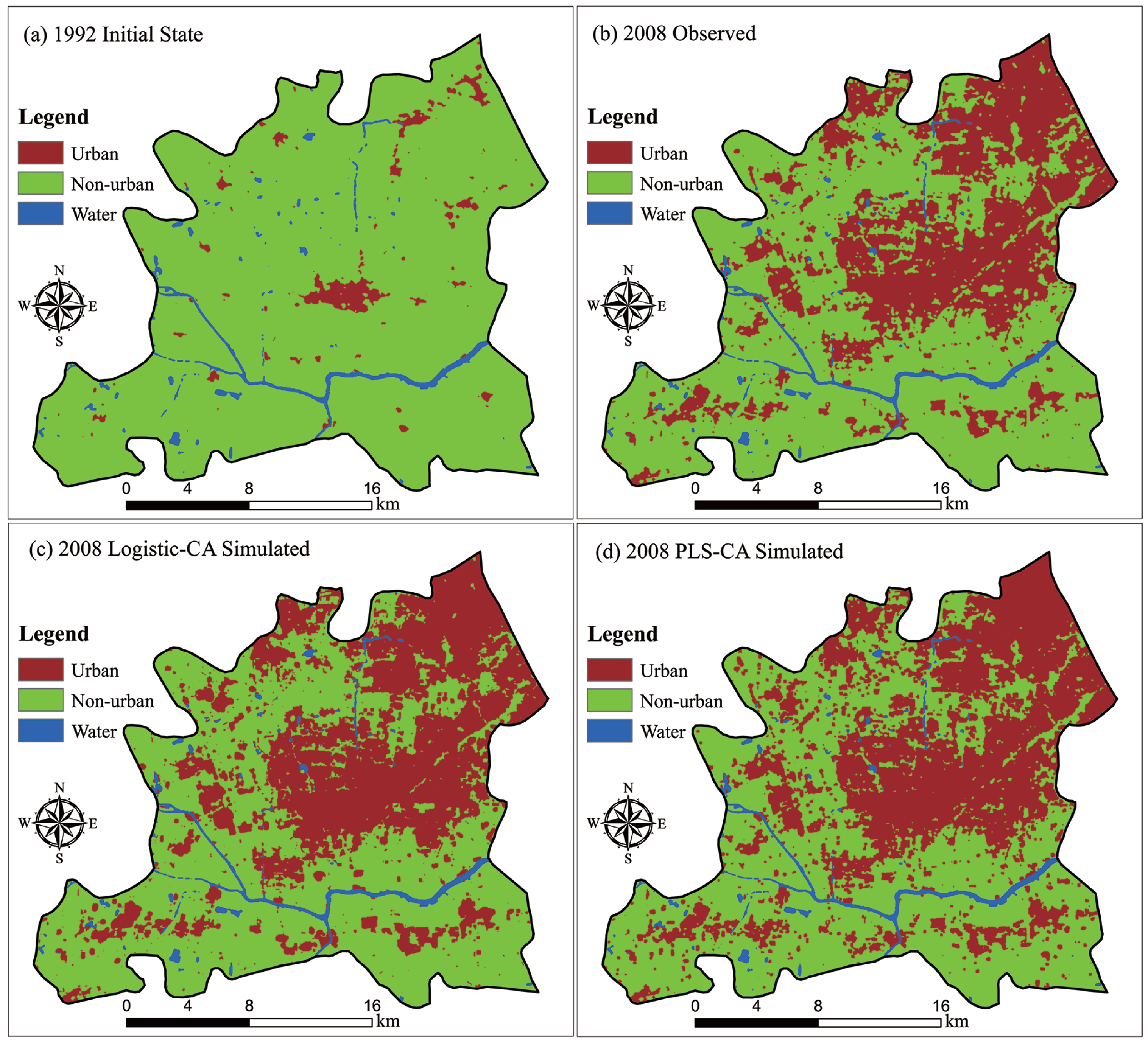
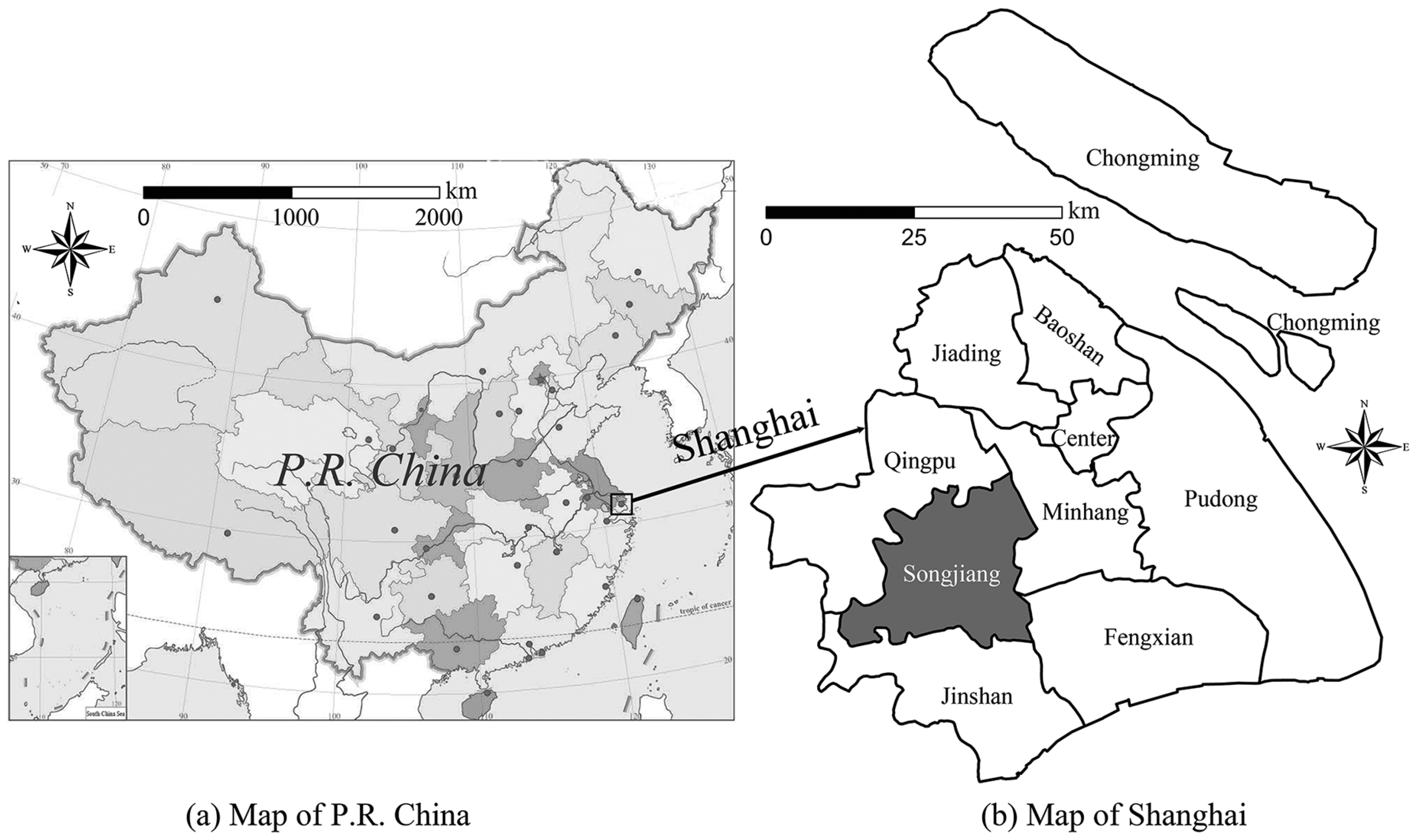
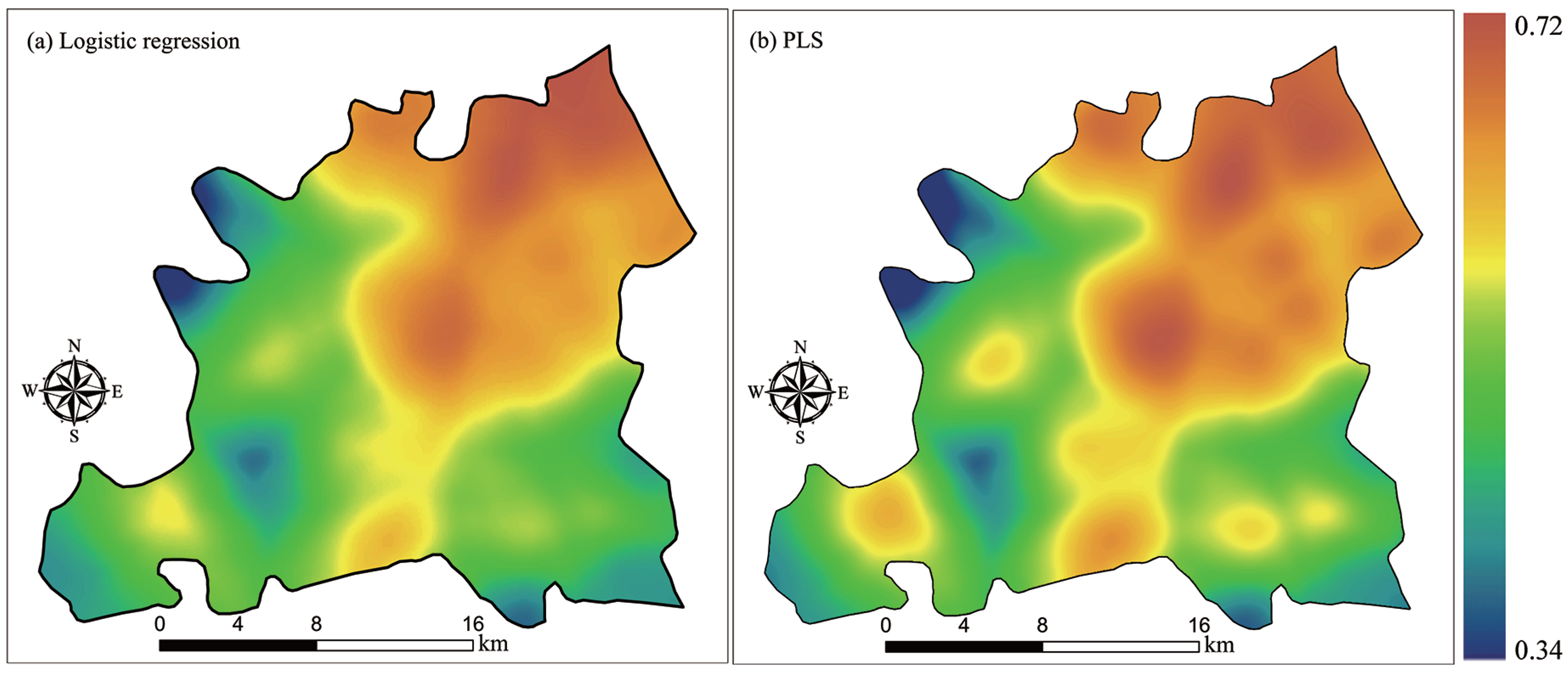
This paper presents a novel CA model based on the PLS approach that we call PLS-CA. This approach was used to derive principal components of the spatial variables for regressing CA parameters. Compared to logistic-CA, PLS can extract variables that are uncorrelated amongst the explanatory variables, and also between the explanatory and response variables. The result is the discovery of important transition rules from a number of driving factors that may be highly correlated. Our PLS-CA model was applied to simulate urban growth in the Songjiang district, an outer suburb of Shanghai Municipality, from 1992 to 2008. For comparison, a logistic-CA model was also applied to simulate the urban growth in the same study area.
3. The PLS-CA Model
3.1. A Generic CA Model
The global conversion probability of land conversion from non-urban to urban can be calculated as the combined effect of the static probability, neighborhood effect, constraints, and random impact [
9,
45]. A general form of the global conversion probabilities for
u × v cells (in a lattice) is:
where
is the global probability of rural-to-urban conversion for cell
ij at time
t;
is the static probability determined by spatial distances [
11,
34];
con() is a constraint function which returns either 0 or 1 [
46];
is the effect for cell
ij at time
t within
neighborhood and it is calculated by
where
returns 1 if the state of the cell
ij is urban, otherwise, it returns 0;
is the stochastic factor [
47], where
Rnd is a random real number ranging from 0 to 1, and
is a parameter ranging from 0 to 10 that adjusts the influence of the stochastic factor.
The global conversion probability, therefore, consists of: (1) the conversion probability based on spatial variables, (2) cell conversion constraints including planning regulation, protected farmland, and water bodies, (3) neighborhood effects, and (4) a stochastic factor. The first component is the observed conversion probability
Pd [
18,
41]:
where
represents the comprehensive impacts of distance-based variables on cell
ij,
are the distances from the cell
ij to a key point such as the urban center, town centers, main roads, etc.; and
are their corresponding parameters. These distances are also defined as spatial or independent variables in our CA modeling.
3.2. The PLS Method
We assume that is a set of dependent variables (i.e., the observed rural-to-urban conversion), where n is the size of samples and q is the number of dependent variables, is a set of independent variables with p as the number of independent variables. We also assume that and are the normalized (mean-centered and variance-scaled) matrix forms of x and y, respectively, is the first principal component vector of , i.e., , is the corresponding unit weight vector of and , and that is the first principal component vector of , i.e., , is the corresponding unit weight vector of and .
In PLS regression, the goal is to obtain a first pair of vectors
and
under the condition that
and
, and maximizing
. The objective can be re-written as an optimization problem [
36,
37]:
By applying the Lagrange algorithm, we obtained eigenvalue equations resolving a first pair of weight vectors
and
as follows:
where
and
are the unit eigenvectors of the matrices
and
, respectively,
is the corresponding eigenvalue, and
. According to Equation (1),
is supposed to be maximal in the sense of PLS regression.
We compute the first pair of component vectors
and
, and run the regression of
and
with respect to
and
, respectively. The equation is:
where
and
are the residual matrices, and
and
are the coefficient vectors that can be given by:
Substituting the residual matrices
and
for
and
and repeating the above method, we obtained the second component vectors
and
as:
where
and
are the unit eigenvectors of matrices
and
respectively, corresponding to the maximum eigenvalue
.
Running the regression of
and
with respect to
and
, respectively, we have:
where the coefficient vectors
and
are calculated from:
The procedure is iterated until
becomes a null matrix, and the final components
are determined by cross-validation. Therefore, we have the following equations:
Since
can be represented as the linear combination of the original variables
, and
in Equation (10) is recovered by the regression equation of
with respect to
as follows:
where
are the corresponding coefficients and
Fmk is the
kth column of residual matrix
Fm.
Cross-validation checks the contributions of the extracted principal components to determine how well the regression model predicts the data. The cross-validation for the component
tn is:
where
PRESSh is the sum of squares of prediction error with a total of
h components (
t1, …,
th), and
SSh−1 is the sum of squares of combination error of
y with the first (
h−1) components (
t1, …,
th−1).
If
, the contribution margin of the newly added component
tn is significant, and as a result, iteration stops when
[
36,
37].
3.3. PLS-Based CA Model
Since the conversion probability of each cell in CA is a single decimal variable, Equation (11) can be re-written as [
36,
37]:
where
is the
regression estimator.
The form of Equation (13) retrieved by PLS method is similar to that from PCA method but the regression estimator
αp obtained from the PLS method contains information about the dependent variable
y as shown in Equation (7), while
αp obtained by PCA does not contain any contribution of the responsive variable
y [
34,
36,
37]. Although data redundancy can be eliminated by PCA, the regression estimators obtained are not related to the independent variables and, thus, have less strong ability to interpret the independent variable
y. PLS is more robust than PCA at explaining the responsive variable
y.
Integrating Equations (1), (2) and (13), we derived the global conversion probability in the PLS-CA model:
If the calculated global probability
exceeds the predefined threshold ranging from 0 to 1, the cell
ij at time
t will be converted to urban land use at time
t + 1. Otherwise, it will retain its current state at next time
t + 1 [
18,
41].
3.4. Structure of the PLS-CA Model
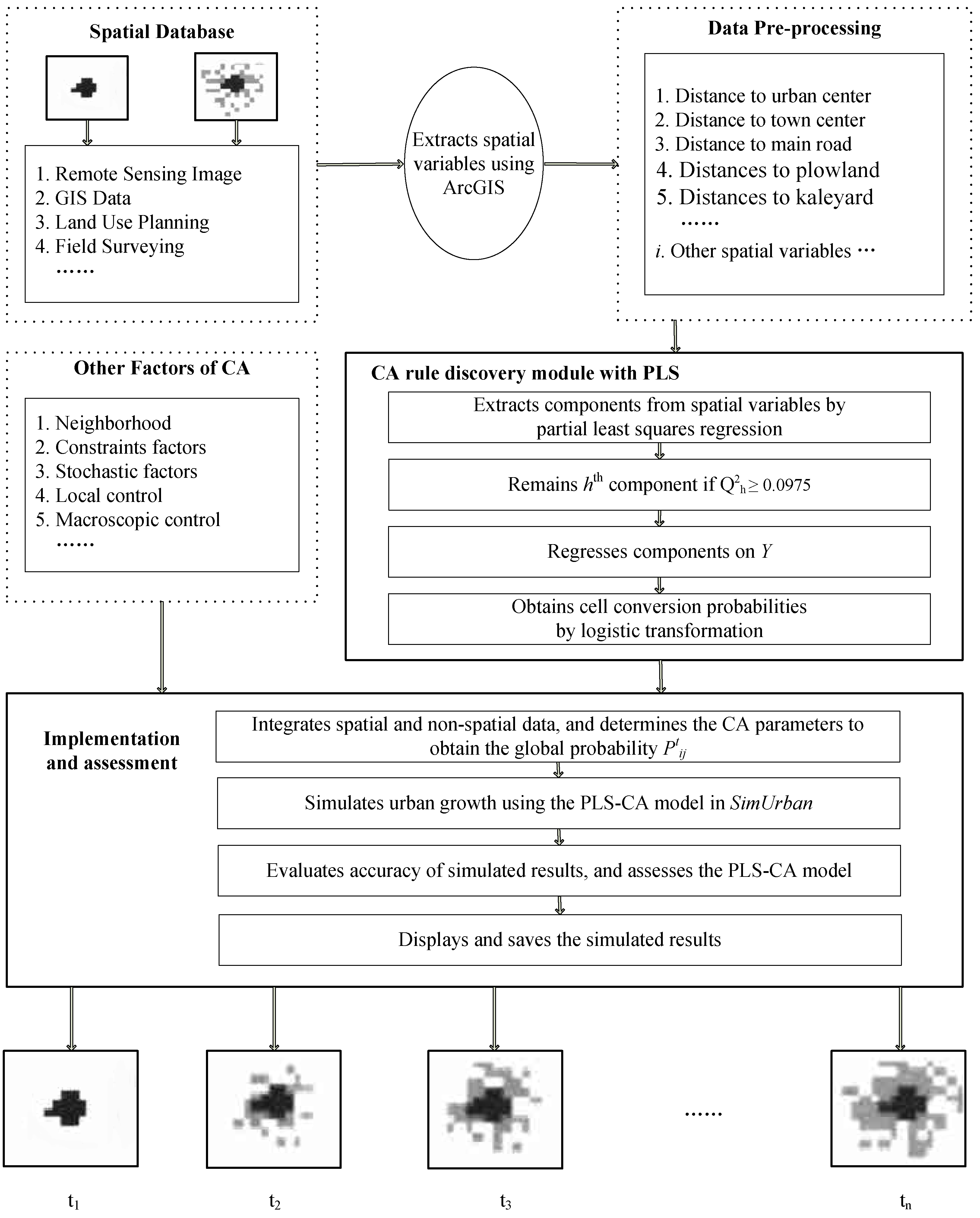
The PLS-CA model workflow consists of five steps: raw data collection, data processing, CA rule discovery with PLS, determination of other CA factors, and model implementation and results assessment (
Figure 3). Each step of the model plays a distinct role in the modeling as follows:
(1) Raw data collection: Data used in the model include historical raster images such as remotely sensed images, an administrative vector map, a topographic map, and a transportation map.
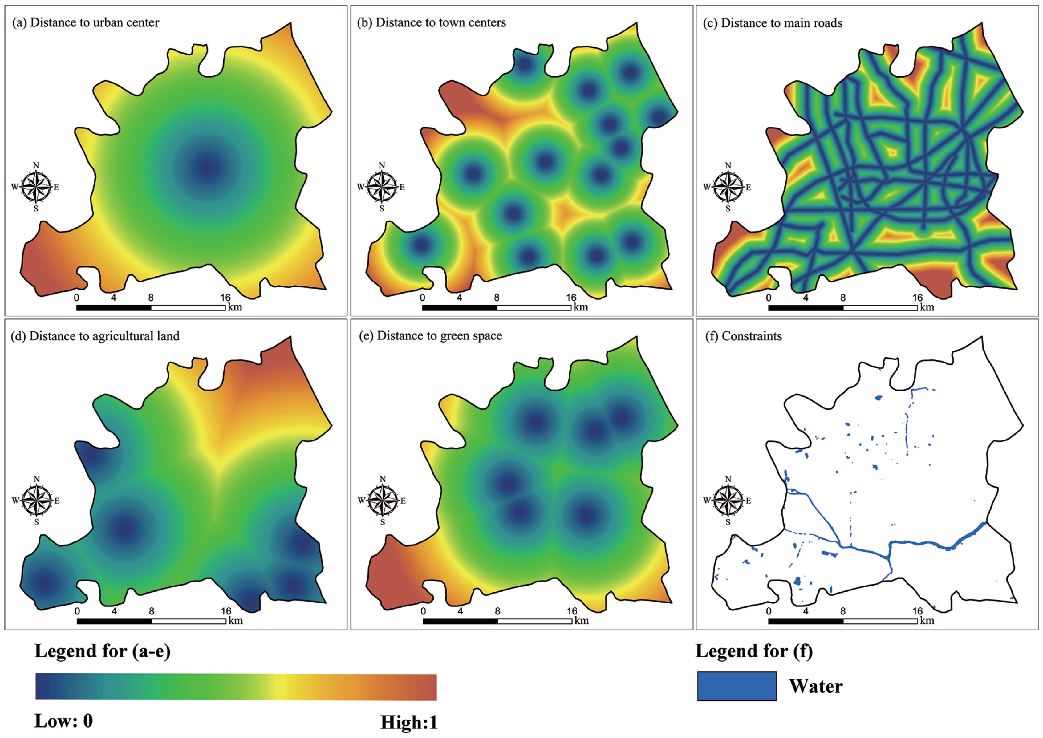
(2) Data processing: Spatial variables were extracted from raw data using the ArcGIS Spatial Analyst tool. These spatial variables included the distance to the urban center (
Durban), town centers (
Dtown), main roads (
Dmrd), agricultural land (
Dagri), and green space (
Dgs). The five spatial variables were normalized by:
where
Dmax is the maximum value of the spatial variable,
Dori is the original distance value from the raw data, and
Dnorm is the normalized value in the range (0, 1). Normalization enables a precise interpretation of the geographic meaning of the parameters. For instance, if a cell is situated at the urban center, its normalized
Durban value will be 0, where if the cell is situated far from the urban center, its normalized
Durban will approach 1.
(3) CA rule discovery: This module derives uncorrelated spatial components using PLS. It determines whether the derived spatial variables satisfy the cross-validation of
and, hence, it is used to define CA parameters (i.e., weights of spatial variables) by which the land conversion probability
under variables can be obtained. The PLS regression was conducted using the “PLSR” package of R-language [
48].
(4) Other CA factors: These include non-spatial factors such as neighborhood effect, constraints of basic farmland, and a stochastic factor.
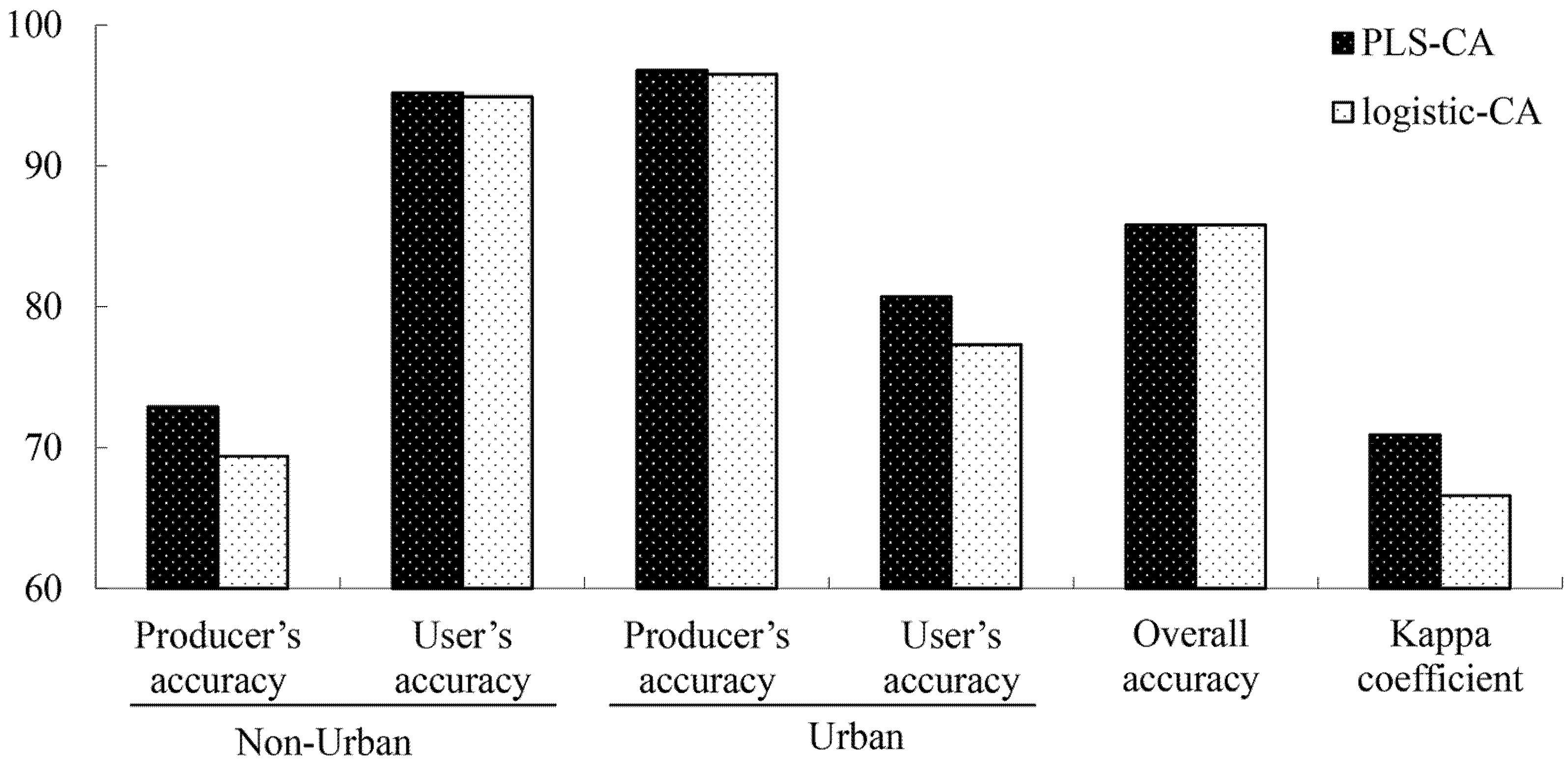
(5) PLS-CA implementation and assessment: This module enables the simulation of the PLS-CA model and incorporates simulation accuracy assessment by generating overall accuracy, producer’s accuracy, user’s accuracy, Kappa coefficient, and the compared urban growth rate (CUGR). The module also displays and exports simulation outcomes.
The simulated area of each category from the CA modeling was not exactly equal to the actual area. Therefore, an indicator termed the compared urban growth rate (
CUGR) is calculated to assess the accuracy of the PLS-CA model by comparing the observed and simulated urban growth rates. The
CUGR indicator was computed as:
where
CUGR is the difference between the observed and simulated areas of each category in terms of growth rate,
Ssim2008 is the simulation area of the urban or non-urban category at 2008, and
Sobs2008 is the statistical areas of observed urban growth in 2008 or non-urban loss in 1992, respectively.
5. Conclusions
This paper demonstrates that CA models can accurately simulate urban growth using global and local constraints that reflect various environmental concerns. The advantages of urban growth simulation by GIS-based CA modeling include the identification of the driving factors of land use change and the identification of spatial patterns across space and over time. The most important part of developing these new models is to discover mature CA transition rules. Our PLS-CA model is capable of extracting uncorrelated factors from the candidate explanatory variables. Thus, PLS-CA can well eliminate redundancy of the input data and, thus, allow for the discovery of better and more reasonable transition rules. The PLS-CA model was successfully applied to simulate the urban growth in Songjiang, demonstrating better simulation accuracy than a conventional logistic-CA model.
Further improvements could be made by testing the response and robustness of the PLS-CA model on sampling, neighborhood configuration, constraints, and spatial scale. In addition, advanced CA models could be packaged with simple, robust, and easily implementable modules such as real-time and dynamic display of simulation results.


