Predicting Relevant Change in High Resolution Satellite Imagery

Abstract

With the ever increasing volume of remote sensing imagery collected by satellite constellations and aerial platforms, the use of automated techniques for change detection has grown in importance, such that changes in features can be quickly identified. However, the amount of data collected surpasses the capacity of imagery analysts. In order to improve the effectiveness and efficiency of imagery analysts performing data maintenance activities, we propose a method to predict relevant changes in high resolution satellite imagery based on human annotations on selected regions of an image. We study a variety of classifiers in order to determine which is most accurate. Additionally, we experiment with a variety of ways in which a diverse set of training data can be constructed to improve the quality of predictions. The proposed method aids in the analysis of change detection results by using various classifiers to develop a relevant change model that can be used to predict the likelihood of other analyzed areas containing a relevant change or not. These predictions of relevant change are useful to analysts, because they speed the interrogation of automated change detection results by leveraging their observations of areas already analyzed. A comparison of four classifiers shows that the random forest technique slightly outperforms other approaches.

1. Introduction

With the proliferation of readily accessible high resolution satellite imagery, many researchers have focused their efforts on multi-temporal imagery analysis. Bhatt and Wallgrun astutely observe that the temporal aspect of spatial data has become an increasingly important component for analysis applications [1], including image to image change detection. One example of such a system is the Geospatial Change Detection and Exploitation System (GeoCDX), a fully-automated system for large-scale change detection in high resolution imagery [2], which was recently published in a Special Issue on multi-temporal analysis of remote sensing data [3]. Other approaches for high resolution change detection include using neural networks [4], hierarchical clustering [5,6], expectation maximization level sets [7], morphological attribute profiles [8] and segmentation [9]. However, in many cases, simply identifying the changes that have occurred is not sufficient.

Several change detection approaches focus the identification of change for very specific purposes. A sampling of these includes mapping land cover patterns for urban growth modeling [10], identifying areas in need of vegetation cover rehabilitation [11] and estimating seismic risk [12]. In this manuscript, we are interested in permanent, anthropogenic changes; a more detailed description is provided in Section 3.1.

We propose an approach for automatically identifying relevant change using a classifier that has been trained with user-identified examples of relevant change. If a user views exemplar regions of a pair of multi-temporal images and provides an assessment of whether or not a relevant change occurred, then we should be able to train a system to then classify other regions within the image.

In previous work, we developed a query-by-example (QBE) system for content-based image retrieval (CBIR) [13–15] that could identify imagery in a database that matched a given query image. In [16], Barb and Kilicay-Ergin developed semantic models using genetic optimization of low-level image features. Other examples of applying data mining algorithms to remote sensing imagery include mining temporal-spatial information [17] and using association rules to extract information from the gaze patterns of individuals viewing satellite imagery [18].

In this manuscript, Section 2 presents a high-level overview of the GeoCDX change detection system, as this serves as the source of the imagery features and change annotations used in the prediction of relevant change. Our definition of relevant change is given in Section 3 along with a description of the classification algorithms used. Section 4 describes the experiments performed to evaluate the change prediction algorithms and discusses the meaning of the results. Finally, Section 5 provides a conclusion and a brief description of future directions of research.

2. Change Detection with GeoCDX

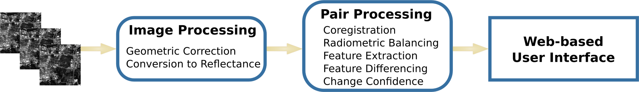
The Geospatial Change Detection and Exploitation System (GeoCDX) is a sensor-agnostic change detection system for high resolution remote sensing imagery [2]. GeoCDX automatically ingests imagery from a variety of sensors, including IKONOS, QuickBird, GeoEye-1 and WorldView-2. Once ingested into the system’s catalog, a data-specific processing plan is developed based on the characteristics of the imagery. The first step of this processing may involve steps, such as geometric correction and conversion to top-of-atmosphere (TOA) reflectance, if they are appropriate for the imagery. The system automatically determines which temporal pairs of images can be created when new imagery is ingested; this also creates a processing plan for each pair. This fully-automated plan includes image-to-image coregistration, radiometric balancing, high-level feature extraction, differencing of the extracted features and fusion of the difference images into a single change confidence image. A summary of these processing steps can be found in Figure 1.

The change detection results are then subdivided by the GeoCDX system into 256 × 256-meter tiles. A per-tile change score is then calculated for each tile based on the extent and intensity of the change. As defined in [2], this per-tile change score is:

$$\frac{1}{\left|\mathit{T}\right|}\left({\displaystyle \sum _{\forall (i,j)\in \mathit{T}}{s}_{ij}}\right)$$

(1)

where T is the set of pixels that compose a tile and s_ij is a per-pixel change score calculated using a non-linear stack filter algorithm that accounts for the intensity and morphological characteristics of the change present at each pixel. This per pixel-change score is described in detail in Section IV.B. of [2].

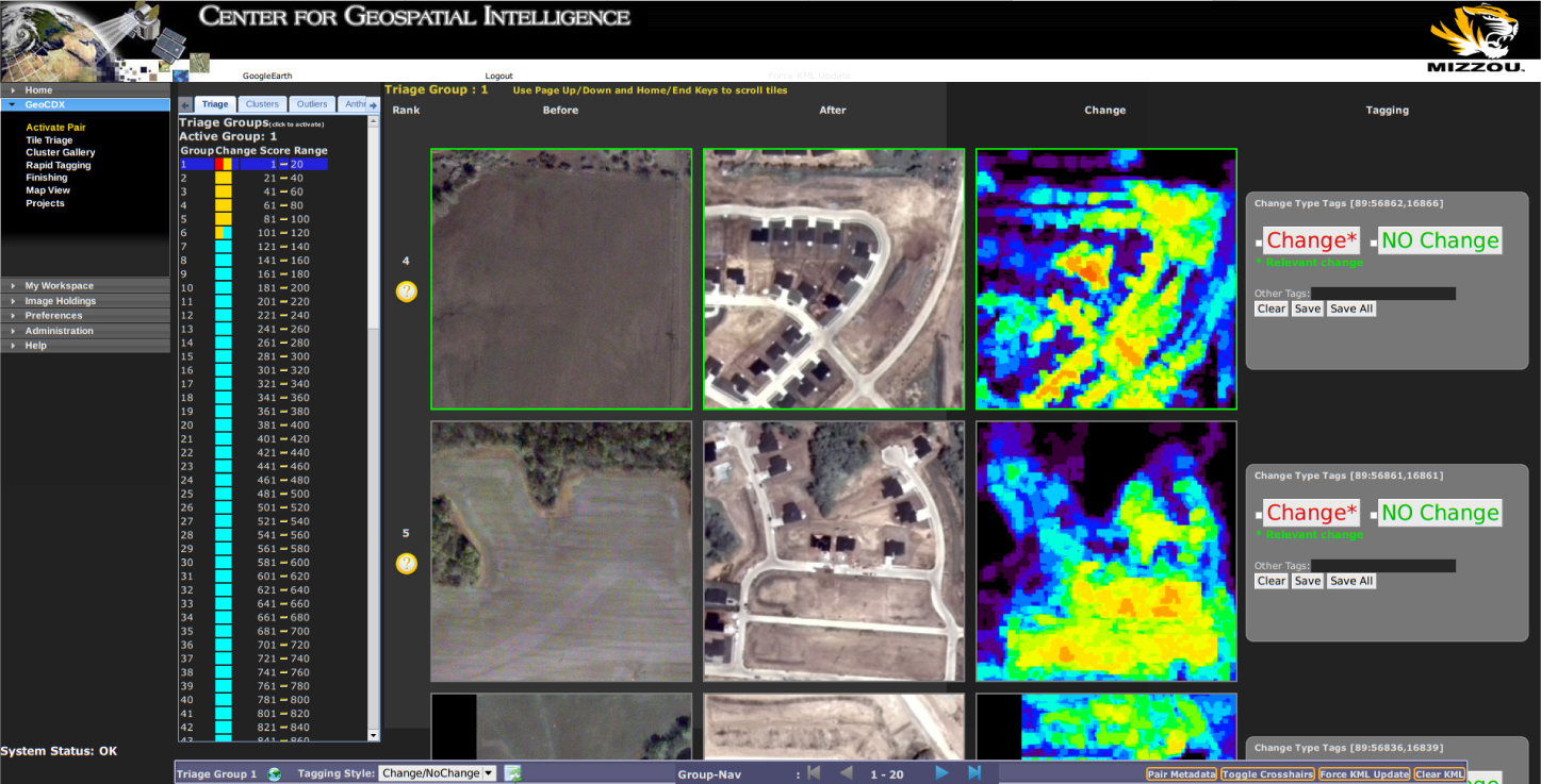
Tiles are then ranked using this change score from most change to least change and presented in rank order in a web interface. Users are then free to exploit the tiles that have been determined to have the most change and stop their analysis when they no longer find a relevant change in the results. An example of highly-ranked change results in the GeoCDX web interface can be seen in Figure 2.

Additionally, the GeoCDX system also uses the per-tile feature signature and per-tile change signature to cluster tiles based on their amount of change and the content. Complete details on the competitive agglomerative clustering algorithm used for this task can be found in [19]. This algorithm produces a dynamic (but bounded) number of clusters based on the degree of variance in the types of change present in a given pair. Each cluster produced represents a distinct type of transition between land-cover, land-use types. For example, one cluster may represent grassland that has changed to residential housing, while another may contain examples of new buildings appearing in urban areas. Figure 3 shows several examples of members of clusters produced by the GeoCDX system.

For the work presented herein, the GeoCDX system was used to perform change detection on imagery from a variety of geographic areas. One of the results (and the only one considered in this work) of the automated GeoCDX change detection processing is a prioritized list of tiles 256 × 256 meters in size that are ordered in terms of most change to least change. In typical usage, an analyst would interrogate these results in rank order, making a change versus no change assessment for each tile. As a user progresses through the list of tiles, we seek to leverage knowledge from the tiles that have already been assessed to make predictions about the remaining tiles in the list that contain change or not.

3. Using Classifiers to Predict Relevant Change

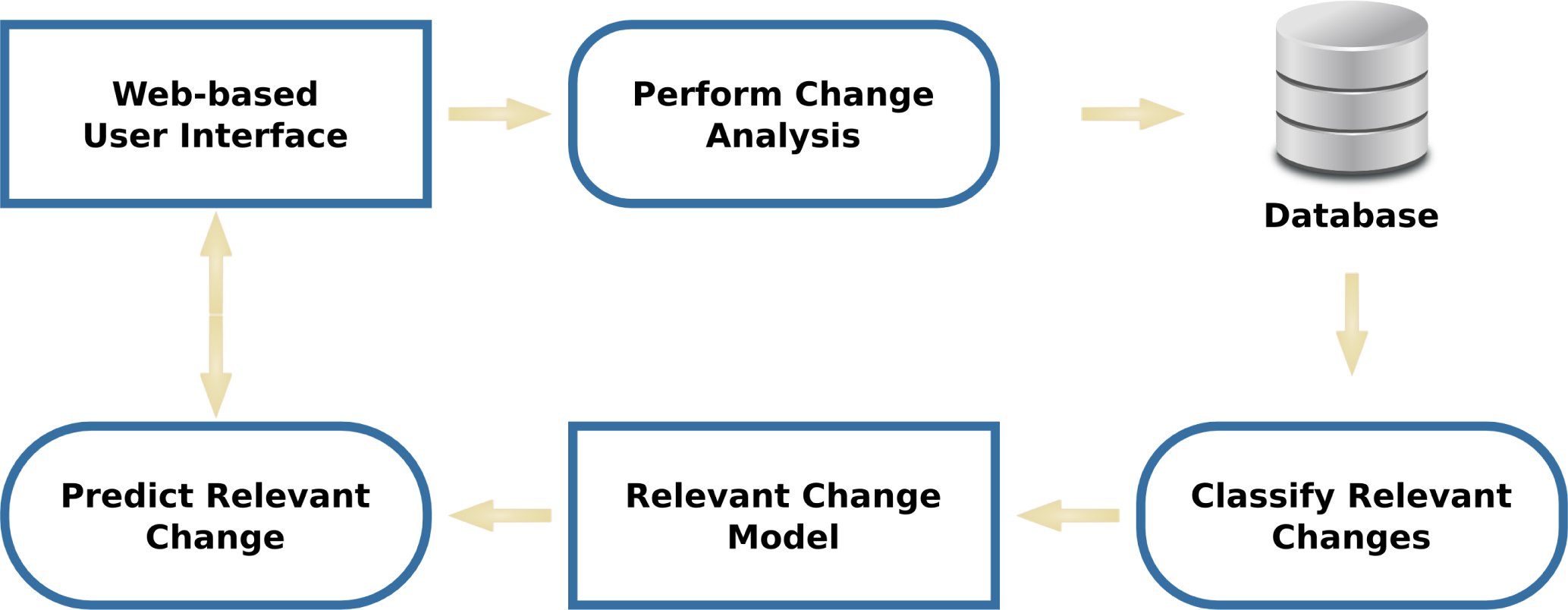
Using the same per-tile feature signatures that the GeoCDX system uses to organize image tiles into clusters [19], we propose methods for predicting areas of relevant change based on prior, manual classification of a subset of a pair. A high-level flow chart of the proposed change prediction methodology can be seen in Figure 4.

A user begins by inspecting tiles in the GeoCDX user interface and performing change analysis to determine if a relevant change has occurred within the tile. These change/no-change annotations are recorded on a per-tile basis in the system database. If change occurs, but is not relevant, it is to be marked as no-change by the analyst. This information can then be used in conjunction with the per-tile features used for change clustering that were described in Section 2 and explained in detail in Section III.A. of [19]. These features are 16-bin histograms that encode information about the 14-pixel level features used by the GeoCDX system. As was the case in [19], we concatenate these histograms together to construct a single feature vector that represents the signature for each tile. We use these signatures along with accumulated change/no change annotation data for a pair to produce a classifier (i.e., the relevant change model) that can be used to predict relevant change for the remaining tiles within a pair.

3.1. Definition of Relevant Change

There are many applications that call for the use of automated change detection using remotely-sensed imagery. Each application has its own set of criteria that define types of changes that are relevant and not relevant. For example, following a natural disaster, emergency management authorities are likely only interested in identifying areas that have been damaged or destroyed. Additionally, insurance companies have an interest in knowing about changes to properties for which they underwrite policies (e.g., expansions of existing structures, new outbuildings being constructed, etc.)

Bruzzone and Bovolo propose a taxonomy of the causes of changes in [20]. In this paper, we propose a scenario in which we are interested in the subset of anthropogenic changes that may require features on a map to be updated that are considered relevant change; all other features are not considered relevant change. Within this definition of relevant change, we include any new building or an extension to an existing building that is at least 200 square meters in area (i.e., approximately the size of a small residential house). Additionally, we consider any new road, parking lot or other impervious surface to be a relevant change. The demolition of any existing building or road is also considered to be a relevant change. Finally, disturbed earth that has been cleared for non-agricultural purposes (e.g., construction, deforestation, etc.) is considered to be relevant change.

Conversely, seasonal or transitory changes are not considered to be relevant changes for this particular experiment. For example, vehicles in parking lots or on roads, although a common sight, are not considered to be a relevant change. Changes to road surfaces, such as repaving, do not constitute a relevant change, because it is not a change that would require an update of features on a map. Agricultural changes (including planting crops, plowing fields, etc.) and seasonal water body fluctuations are not relevant for this experiment. Finally, ephemeral changes, such as shadows or building glint (due to over-saturation of the sensor), leading to streaking, is not a relevant change.

3.2. Classification Algorithms

In this manuscript, we present change classification results from four different algorithms in order to determine the relative efficacy of each. The input to each classification model is a real-valued feature vector along with a binary (change/no-change) classification for each training data point. For classification purposes, we use the same feature vectors used to cluster the tiles that were described in Section 2. From this training dataset, a classification model is built for nearest neighbor, SVM, decision tree (CART) and random forest classification.

3.2.1. k-Nearest Neighbors

The simplest algorithm employed in this manuscript is the k-nearest neighbors classification algorithm [21]. For a given tile to be classified, its feature vector, x, is compared to those of all training tiles in the set and the class of the nearest tile in the feature space is assigned.

3.2.2. Support Vector Machines

The use of support vector machines (SVMs) has been widely discussed as a means of performing nonlinear two-class classification. Originally developed by Cortes and Vapnik [22], SVMs are capable of performing efficient classification of data not otherwise linearly separable by employing the “kernel trick” to project data into a high-dimensional feature space.

For each tile in the training set, we can define feature vector x_i∈ R_d and assignment membership to it based on whether it was marked as being relevant change (i.e., let y_i = 1) or either not-relevant change or no change (i.e., let y_i = −1). If we let w represent the vector normal to the hyperplane that divides the two sets, then we can solve the classification problem using quadratic programming. We must optimize:

$$\underset{(\mathbf{w},b)}{\mathrm{argmin}}\frac{1}{2}\left|\right|\mathbf{w}|{|}^2$$

(2)

subject to:

$$y_i(\mathbf{w}*{\mathbf{x}}_{\mathbf{i}}-b)\ge 1$$

(3)

for all values of i. The resulting classification is the one which maximizes the margin, or separation between the two classes, in the high dimensional space used by the chosen kernel.

Classification is then performed by projecting each new data point into the same high dimensional space and determining on which side of the hyperplane it falls.

3.2.3. Decision Tree Classification

Additionally, we employ the CART decision tree classification algorithm originally proposed by Breiman et al. [23]. Decision trees are a non-parametric technique that are built by making choices at each node in the tree regarding how to split the dataset in such a way that balances the data points and yields the greatest predictive accuracy. These splits continue recursively until each node contains data points belonging to a single class or some predetermined node size has been reached.

Classification can be performed by starting at the root node and walking the decision tree until a node is reached. A class label is then assigned based on the label of the data points in the node.

3.2.4. Random Forest

The decision tree concept was extended by Breiman to create the ensemble classification method of random forests [24]. This technique utilizes “bagging” to sample the training dataset to produce multiple decision trees. During the classification stage, these trees are then used in concert to produce several classification results. Each tree casts a vote for classification of the data point, and the consensus data point (i.e., the one with the plurality of votes) is assigned.

4. Results

In this section, we will describe the experiments performed to test the predictions of relevant change made by various algorithms. These experiments involved data from the three areas shown in

Table 1. Information about the three image pairs used during the experiments presented herein.

Location	Before Image		After Image		km2	No. of Tiles
	Date	Sensor	Date	Sensor
Columbia, MO, USA	April 30, 2000	IKONOS	June 28, 2006	QuickBird	159	2528
Las Vegas, NV, USA	May 10, 2002	QuickBird	May 18, 2003	QuickBird	31	522
Natanz, Iran	September 19, 2006	QuickBird	June 11, 2007	QuickBird	250	3660

. The regions used were varied in their landscape. Columbia, Missouri, USA, contains a mix of urban areas and rural farmland, both of which showed moderate amounts of change. The Las Vegas, Nevada, USA, imagery was highly urbanized and contained significant amounts of change. Finally, a sparsely-populated, mountainous area near Natanz, Iran, was used, which underwent very little change during the time period between the two images.

In order to generalize well, a classifier should be built with a training dataset that matches the natural distribution of the entire dataset [25]. This is particularly challenging with imbalanced datasets in which there are relatively few samples from one class. Methods to address the challenge of imbalanced datasets can be grouped into three categories [26]: adapting existing algorithms, pre-processing the datasets through sampling techniques or post-processing the classification model. While the Columbia and Las Vegas datasets are split roughly 3:1 between no change and change tiles, the Natanz dataset is split 50:1 between no change and change tiles. Given the potential challenges of our dataset, we will investigate dataset sampling techniques, such as those proposed in [27], to improve our classification results. The following sections describe sampling methods that employ knowledge of the dataset to ensure that a variety of types of data points are included in the training set.

Table 2. Size of training dataset versus testing dataset.

Dataset	Columbia				Las Vegas				Natanz
	Training	Testing			Training	Testing			Training	Testing
	No.	No.	% Change	% No Change	No.	No.	% Change	% No Change	No.	No.	% Change	% No Change
A1	126	2,402	28.18%	71.82%	26	496	20.36%	79.64%	183	3,477	4.80%	95.20%
A2	379	2,149	24.57%	75.43%	78	444	14.19%	85.81%	549	3,111	2.73%	97.27%
A3	632	1,896	21.89%	78.11%	130	392	11.22%	88.78%	915	2,745	1.42%	98.58%
B1	252	2,276	29.53%	70.47%	52	470	21.28%	78.72%	366	3,294	5.07%	94.93%
B2	758	1,770	28.87%	71.13%	156	366	16.39%	83.61%	1,098	2,562	3.32%	96.68%
B3	1,264	1,264	30.06%	69.94%	260	262	15.65%	84.35%	1,830	1,830	2.13%	97.87%
C1	100	2,428	31.05%	68.95%	90	432	25.69%	74.31%	90	3,570	6.75%	93.25%
C2	292	2,236	30.50%	69.50%	256	266	31.95%	68.05%	268	3,392	5.98%	94.02%
C3	477	2,051	29.64%	70.36%	368	154	36.36%	63.64%	441	3,219	5.19%	94.81%
D1	222	2,306	27.93%	72.07%	113	409	22.25%	77.75%	261	3,399	4.62%	95.38%
D2	315	2,213	27.70%	72.30%	203	319	24.76%	75.24%	335	3,325	4.42%	95.58%
D3	407	2,121	27.30%	72.70%	277	245	26.94%	73.06%	410	3,250	4.15%	95.85%
E1	466	2,062	24.35%	75.65%	162	360	15.28%	84.72%	604	3,056	2.59%	97.41%
E2	553	1,975	24.00%	76.00%	246	276	17.03%	82.97%	655	3,005	2.46%	97.54%
E3	636	1,892	23.57%	76.43%	313	209	17.70%	82.30%	710	2,950	2.31%	97.69%
F1	336	2,192	29.20%	70.80%	136	386	23.32%	76.68%	444	3,216	4.88%	95.12%
F2	420	2,108	28.89%	71.11%	224	298	26.17%	73.83%	518	3,142	4.68%	95.32%
F3	500	2,028	28.40%	71.60%	291	231	28.14%	71.86%	593	3,067	4.40%	95.60%
G1	816	1,712	28.50%	71.50%	224	298	17.79%	82.21%	1,153	2,507	3.15%	96.85%
G2	880	1,648	27.91%	72.09%	295	227	20.26%	79.74%	1,204	2,456	3.01%	96.99%
G3	941	1,587	27.41%	72.59%	347	175	20.57%	79.43%	1,259	2,401	2.83%	97.17%

shows the number of training and testing samples used for each dataset as well as the percent of change and no change tiles contained within each testing dataset.

4.1. Predictions Using High-Change Tiles

The first experiment involves using tiles that the GeoCDX system identified as being high change tiles. Using these high change tiles, each of the four classifiers will be trained with the data corresponding to a fixed percentage of tiles. While the selected tiles are all high-change tiles, not all of the change captured by them is necessarily relevant change. We produced three different datasets with high change tiles; they include the highest ranked 5%, 15% and 25% of the dataset.

Table 3. In the Series A datasets, we selected only tiles that were highly ranked. Each row represents a dataset with a different fraction of tiles selected.

Dataset	% of Tiles	No. of High Change Tiles
		Columbia	Las Vegas	Natanz
A1	5%	126	26	183
A2	15%	379	78	549
A3	25%	632	130	915

shows the chosen percentages and the corresponding number of tiles used from each pair.

4.3. Predictions Using Cluster Members

Recall that Section 2 described the clustering of change detection results. In an effort to train the classifier with a more diverse training dataset, we can use these clusters to produce our training samples. As was mentioned above, the number of clusters varies by pair, as does the number of members in each cluster. We began by producing a training dataset for each pair that contained the most representative member of each cluster in the pair. Then, we produced expanded training datasets for each pair by including the second and then third most representative member in each cluster.

Table 5. In the Series C datasets, we utilize the most prototypical cluster members from each pair for training data. Each row in this table shows the number of training tiles used as the number of cluster members is increased.

Dataset	Nos. from Each Cluster	No. of Cluster Tiles for Training			Total % of Tiles
		Columbia	Las Vegas	Natanz	Columbia	Las Vegas	Natanz
C1	1	100	90	90	3.96%	17.24%	2.46%
C2	2	292	256	268	11.55%	49.04%	7.32%
C3	3	477	368	441	18.87%	70.50%	12.05%

shows a summary of the number of tiles used for each dataset.

4.4. Predictions Using Cluster Members in Addition to High- and Low-Change Tiles

Finally, we also produce datasets that combine tiles that have very high GeoCDX change scores, very low GeoCDX change scores and representative exemplars from each GeoCDX change cluster.

Table 6. The D, E, F and G series datasets combine tiles with high and low amounts of change in them with prototypical cluster members to form diverse training datasets.

Dataset	% of High Tiles	% of Low Tiles	Nos. from Each Cluster
D1	5%	0%	1
D2	5%	0%	2
D3	5%	0%	3
E1	10%	0%	1
E2	10%	0%	2
E3	10%	0%	3
F1	5%	5%	1
F2	5%	5%	2
F3	5%	5%	3
G1	15%	15%	1
G2	15%	15%	2
G3	15%	15%	3

and

Table 7. This table provides more detailed information on the composition of the training datasets introduced in Table 6.

Dataset	No. of Tiles			Total % of Tiles
	Columbia	Las Vegas	Natanz	Columbia	Las Vegas	Natanz
D1	222	113	261	8.78%	21.65%	7.13%
D2	315	203	335	12.46%	38.89%	9.15%
D3	407	277	410	16.10%	53.07%	11.20%
E1	466	162	604	18.43%	31.03%	16.50%
E2	553	246	655	21.88%	47.13%	17.90%
E3	636	313	710	25.16%	59.96%	19.40%
F1	336	136	444	13.29%	26.05%	12.13%
F2	420	224	518	16.61%	42.91%	14.15%
F3	500	291	593	19.78%	55.75%	16.20%
G1	816	224	1153	32.28%	42.91%	31.50%
G2	880	295	1204	34.81%	56.51%	32.90%
G3	941	347	1259	37.22%	66.48%	34.40%

show a summary of the composition of these training datasets. Ideally, these tiles depict the wide variety of land cover and land use types present in each pair to address the sampling concerns described in the introduction to Section 4.

4.5. Prediction Results

Using all of the training datasets described in the previous subsections, we will construct a nearest neighbor, support vector machine, decision tree and random forest classifier for each dataset. We will use each classifier to label all of the remaining data (i.e., the test data) and compare the results to ground truth change/no-change labels applied by an experienced imagery analyst. Based on these classification results, we catalog the following:

• true positive results: relevant change occurred, and it was classified as such;

• false positive results: no change occurred or a change that was not relevant occurred, but was classified by the algorithm as change;

• false negative results: a relevant change occurred, but was not correctly classified;

• true negative results: no change occurred or a change occurred that was not relevant, and the classifier correctly indicated this condition.

Based on these four factors, we can calculate traditional assessment metrics of precision and recall as follows:

$$\mathit{Precision}=\frac{\mathit{TP}}{\mathit{TP}+\mathit{FP}}$$

(4)

$$\mathit{Recall}=\frac{\mathit{TP}}{\mathit{TP}+\mathit{FN}}$$

(5)

An accuracy metric can also be calculated to measure the overall performance of each algorithm, as shown in Equation (6).

$$\mathit{Accuracy}=\frac{\mathit{TP}+\mathit{TN}}{\mathit{TP}+\mathit{FP}+\mathit{FN}+\mathit{TN}}$$

(6)

We present four tables that illustrate the precision, recall and accuracy values for each of the types of classifiers described in Section 3.

Table 8. Nearest neighbor change prediction results.

Dataset	Columbia			Las Vegas			Natanz
	Precision	Recall	Accuracy	Precision	Recall	Accuracy	Precision	Recall	Accuracy
A1	28.95%	83.60%	37.55%	21.05%	99.01%	24.19%	5.03%	70.66%	34.54%
A2	26.97%	80.49%	41.65%	14.10%	85.71%	23.87%	2.66%	43.53%	54.87%
A3	23.47%	60.96%	47.94%	11.11%	56.82%	44.13%	1.40%	25.64%	73.26%
B1	34.70%	21.43%	64.89%	27.78%	45.00%	63.40%	6.30%	34.73%	70.52%
B2	35.93%	36.99%	62.77%	20.90%	70.00%	51.64%	3.97%	27.06%	75.84%
B3	36.88%	31.05%	63.29%	16.85%	36.59%	61.83%	2.66%	17.95%	84.26%
C1	40.49%	61.27%	60.01%	44.74%	30.63%	72.45%	9.96%	21.58%	81.54%
C2	37.15%	59.97%	56.84%	40.98%	29.41%	63.91%	7.24%	25.12%	76.27%
C3	39.66%	57.40%	61.48%	44.74%	30.36%	61.04%	7.74%	27.54%	79.22%
D1	35.09%	57.40%	58.33%	38.67%	31.87%	73.59%	5.61%	40.13%	66.08%
D2	32.96%	57.92%	54.50%	37.88%	31.65%	70.22%	5.68%	37.41%	69.77%
D3	32.63%	62.15%	55.73%	35.09%	30.30%	66.12%	4.95%	34.81%	69.54%
E1	28.65%	58.38%	52.96%	22.02%	43.64%	67.78%	2.58%	35.44%	63.78%
E2	28.17%	62.55%	51.59%	27.40%	42.55%	71.01%	2.54%	33.78%	66.42%
E3	28.24%	65.61%	53.86%	20.75%	29.73%	67.46%	2.36%	32.35%	67.63%
F1	39.95%	50.94%	63.32%	40.00%	33.33%	72.80%	5.72%	23.57%	77.30%
F2	36.83%	57.14%	59.30%	37.50%	30.77%	68.46%	5.99%	24.49%	78.49%
F3	35.39%	54.69%	58.78%	34.55%	29.23%	64.50%	5.23%	25.19%	76.62%
G1	38.91%	42.42%	64.60%	27.27%	45.28%	68.79%	3.25%	20.25%	78.46%
G2	37.50%	46.30%	63.47%	29.51%	39.13%	68.72%	3.25%	20.27%	79.44%
G3	36.59%	47.36%	63.07%	21.74%	27.78%	64.57%	3.29%	22.06%	79.43%

provides results for the nearest neighbor classifier,

Table 9. Support vector machine change prediction results.

Dataset	Columbia			Las Vegas			Natanz
	Precision	Recall	Accuracy	Precision	Recall	Accuracy	Precision	Recall	Accuracy
A1	28.19%	99.85%	28.27%	20.53%	100.00%	21.17%	5.13%	100.00%	11.19%
A2	27.02%	91.67%	37.13%	14.40%	88.89%	23.42%	2.55%	30.59%	66.15%
A3	26.96%	76.14%	49.63%	13.17%	61.36%	50.26%	1.05%	5.13%	91.77%
B1	38.55%	34.08%	64.50%	34.52%	29.00%	73.19%	13.30%	17.37%	90.07%
B2	52.86%	36.20%	72.26%	30.70%	58.33%	71.58%	9.38%	3.53%	95.67%
B3	50.83%	32.11%	70.25%	35.29%	29.27%	80.53%	0.00%	0.00%	97.27%
C1	51.11%	36.74%	69.44%	55.88%	17.12%	75.23%	22.95%	5.81%	92.32%
C2	47.15%	41.20%	67.98%	52.94%	31.76%	69.17%	21.05%	5.91%	93.04%
C3	49.73%	46.22%	70.21%	66.67%	53.57%	73.38%	19.15%	5.39%	93.91%
D1	33.09%	71.27%	51.73%	46.15%	19.78%	77.02%	5.97%	29.30%	75.40%
D2	36.89%	61.99%	60.10%	51.02%	31.65%	75.55%	7.94%	14.97%	88.57%
D3	41.77%	59.59%	66.29%	46.51%	30.30%	71.84%	8.95%	12.59%	91.05%
E1	32.39%	70.92%	56.89%	35.29%	32.73%	80.56%	2.22%	16.46%	79.12%
E2	33.96%	64.77%	61.32%	30.95%	27.66%	77.17%	1.95%	10.81%	84.43%
E3	36.00%	62.56%	64.96%	26.32%	27.03%	73.68%	1.83%	7.35%	88.78%
F1	53.60%	45.31%	72.58%	57.89%	24.44%	78.24%	22.22%	8.92%	94.03%
F2	52.79%	46.63%	72.53%	52.27%	29.49%	74.50%	23.08%	6.12%	94.65%
F3	49.64%	47.40%	71.40%	47.62%	30.77%	71.00%	15.79%	4.44%	94.75%
G1	53.60%	45.31%	72.58%	39.53%	32.08%	79.19%	11.54%	3.80%	96.05%
G2	52.79%	46.63%	72.53%	57.89%	24.44%	78.24%	11.54%	4.05%	96.17%
G3	49.64%	47.40%	71.40%	52.27%	29.49%	74.50%	9.52%	2.94%	96.46%

for support vector machine,

Table 10. Decision tree (CART) change prediction results.

Dataset	Columbia			Las Vegas			Natanz
	Precision	Recall	Accuracy	Precision	Recall	Accuracy	Precision	Recall	Accuracy
A1	31.91%	93.94%	41.80%	20.36%	100.00%	20.36%	4.91%	87.43%	18.03%
A2	29.03%	79.55%	47.18%	17.41%	74.60%	46.17%	2.86%	63.53%	39.99%
A3	27.67%	69.40%	53.59%	12.13%	75.00%	36.22%	2.04%	64.10%	55.81%
B1	42.34%	41.96%	65.99%	75.00%	18.00%	81.28%	6.86%	38.32%	70.49%
B2	42.48%	41.49%	66.89%	45.83%	18.33%	83.06%	5.76%	22.35%	85.28%
B3	38.99%	22.37%	66.14%	75.00%	7.32%	85.11%	4.00%	10.26%	92.84%
C1	44.03%	56.23%	64.21%	64.95%	56.76%	81.02%	7.67%	36.10%	66.36%
C2	46.19%	42.67%	67.35%	76.74%	38.82%	76.69%	8.10%	38.92%	69.93%
C3	42.67%	53.13%	64.94%	43.40%	41.07%	59.09%	5.28%	25.75%	72.20%
D1	40.06%	65.68%	62.97%	45.05%	45.05%	75.55%	4.78%	46.50%	54.75%
D2	38.17%	53.18%	63.17%	64.58%	39.24%	79.62%	5.38%	46.26%	61.62%
D3	37.80%	54.06%	63.18%	50.00%	42.42%	73.06%	5.60%	40.74%	69.02%
E1	34.43%	60.56%	62.32%	42.86%	16.36%	83.89%	3.07%	59.49%	50.36%
E2	35.37%	57.38%	64.61%	52.94%	38.30%	83.70%	2.92%	51.35%	56.71%
E3	34.29%	58.74%	63.74%	27.59%	43.24%	69.86%	2.81%	54.41%	55.59%
F1	50.40%	39.69%	70.99%	45.05%	45.56%	74.35%	7.25%	26.75%	79.73%
F2	41.84%	50.90%	65.37%	64.58%	39.74%	78.52%	6.26%	24.49%	79.31%
F3	39.17%	53.99%	63.12%	49.15%	44.62%	71.43%	5.88%	23.70%	79.95%
G1	40.31%	43.03%	65.60%	43.75%	13.21%	81.54%	5.12%	21.52%	84.96%
G2	43.87%	45.87%	68.51%	40.00%	13.04%	78.41%	3.50%	14.86%	85.10%
G3	39.87%	42.53%	66.67%	34.21%	36.11%	72.57%	4.17%	16.18%	87.09%

for the decision tree and

Table 11. Random forest change prediction results.

Dataset	Columbia			Las Vegas			Natanz
	Precision	Recall	Accuracy	Precision	Recall	Accuracy	Precision	Recall	Accuracy
A1	28.18%	100.00%	28.18%	20.40%	100.00%	20.56%	4.98%	94.61%	13.00%
A2	28.09%	93.37%	39.65%	14.36%	93.65%	19.82%	2.94%	80.00%	27.32%
A3	26.07%	84.82%	44.04%	13.47%	75.00%	43.11%	2.31%	69.23%	57.92%
B1	47.46%	48.66%	68.94%	60.61%	20.00%	80.21%	16.67%	5.39%	93.84%
B2	47.70%	36.59%	70.11%	33.33%	15.00%	81.15%	100.00%	1.18%	96.72%
B3	48.33%	30.53%	69.30%	50.00%	7.32%	84.35%	100.00%	2.56%	97.92%
C1	56.25%	32.23%	71.17%	100.00%	2.70%	75.00%	12.50%	3.32%	91.90%
C2	55.38%	31.67%	71.38%	100.00%	1.18%	68.42%	22.41%	6.40%	93.07%
C3	56.06%	42.60%	73.09%	100.00%	12.50%	68.18%	22.00%	6.59%	93.94%
D1	35.41%	88.20%	51.78%	76.92%	10.99%	79.46%	5.94%	66.88%	49.54%
D2	41.53%	71.94%	64.17%	100.00%	6.33%	76.80%	5.28%	25.85%	76.21%
D3	46.27%	62.18%	69.97%	100.00%	12.12%	76.33%	8.86%	20.74%	87.85%
E1	31.01%	85.06%	50.29%	31.82%	12.73%	82.50%	3.19%	64.56%	48.40%
E2	34.24%	77.43%	58.89%	37.50%	6.38%	82.25%	2.80%	37.84%	66.16%
E3	36.67%	66.59%	65.01%	33.33%	5.41%	81.34%	3.43%	33.82%	76.54%
F1	51.84%	52.81%	71.90%	80.00%	8.89%	78.24%	40.00%	2.55%	95.06%
F2	53.55%	53.20%	73.15%	100.00%	8.97%	76.17%	75.00%	2.04%	95.39%
F3	52.58%	51.39%	73.03%	100.00%	13.85%	75.76%	100.00%	2.22%	95.70%
G1	48.83%	38.52%	70.97%	25.00%	3.77%	80.87%	100.00%	1.27%	96.89%
G2	50.14%	40.22%	72.15%	33.33%	4.35%	78.85%	100.00%	1.35%	97.03%
G3	49.58%	40.92%	72.40%	40.00%	5.56%	78.86%	100.00%	1.47%	97.21%

for the random forest classifier. Each row in the table corresponds to one of the training datasets described in Tables 3–5, 6 and 7.

Table 8 shows the results of change prediction using a nearest neighbor classifier. Recall rates are highest when only using the high change tiles as training data (Datasets A1–A3); this holds true for all three test sites. However, when using this training data, overall accuracy clearly suffers. Generally, the highest combinations of precision, recall and accuracy values come from the training datasets that combine high change tiles and members from each of the change clusters (the F and G series datasets). However, overall, the results of using a nearest neighbor (NN) classifier are not compelling.

Results that quantify the performance of support vector machine (SVM) classification can be found in Table 9. Overall, these results show a marked improvement over those of the NN classifier. Again, the use of training sets that combine high change tiles with representative cluster members continue to produce the best classification results. Precision and accuracy values hover around the 50% mark, while overall accuracy is between 70–80% for the Columbia and Las Vegas datasets. The Natanz dataset represents an anomaly, because of the relatively small amount of actual change in the dataset; precision and recall values typically top out no higher than 30%, but overall accuracy is in the mid-90% range. This occurs because the classifier is able to accurately predict a large number of true negative tiles within this pair.

Generally, the results of the CART decision tree classification shown in Table 10 indicate a slight decrease in precision, recall and accuracy compared to those of the SVM. The notable exception was that the D and E series datasets showed a slight improvement using the CART decision tree compared to SVM.

Finally, change prediction results using the random forest classifier shown in Table 11 are the best among the four algorithms presented.

4.6. Analysis of Results Using a Generalized F-Score

The F-score is a commonly-used assessment to determine a classification algorithm’s accuracy in a way that takes into account both precision and accuracy. The traditional F₁ score is calculated as the harmonic mean of the precision and recall values and is bounded between zero and one. F₁ can be calculated as follows:

$${\mathit{F}}_1=2\cdot \frac{\mathit{Precision}\cdot \mathit{Recall}}{\mathit{Precision}+\mathit{Recall}}=\frac{2\cdot \mathit{TP}}{2\cdot \mathit{TP}+\mathit{FP}+\mathit{FN}}$$

(7)

where TP represents the number of true positive outcomes, FP the number of false positive outcomes and FN the number of false negative outcomes.

A more generalized version of the F-score can be calculated by introducing a variable β that allows more emphasis to be placed on the precision or recall component. This generalized F-score, Fβ, is calculated as:

$${\mathit{F}}_{\mathit{\beta }}=(1+{\mathit{\beta }}^2)\cdot \frac{\mathit{Precision}\cdot \mathit{Recall}}{{\mathit{\beta }}^2\cdot \mathit{Precision}+\mathit{Recall}}$$

(8)

where a larger value of β weights recall more highly than precision and a smaller value of β emphasizes precision at the expense of recall.

Table 12. Analysis of nearest neighbor change prediction results using a generalized F-Score.

Dataset	Columbia			Las Vegas			Natanz
	F0.1	F1	F10	F0.1	F1	F10	F0.1	F1	F10
A1	0.29	0.43	0.82	0.21	0.35	0.96	0.05	0.09	0.63
A2	0.27	0.40	0.79	0.14	0.24	0.82	0.03	0.05	0.38
A3	0.24	0.34	0.60	0.11	0.19	0.55	0.01	0.03	0.22
B1	0.34	0.26	0.22	0.28	0.34	0.45	0.06	0.11	0.33
B2	0.36	0.36	0.37	0.21	0.32	0.68	0.04	0.07	0.26
B3	0.37	0.34	0.31	0.17	0.23	0.36	0.03	0.05	0.17
C1	0.41	0.49	0.61	0.45	0.36	0.31	0.10	0.14	0.21
C2	0.37	0.46	0.60	0.41	0.34	0.29	0.07	0.11	0.25
C3	0.40	0.47	0.57	0.45	0.36	0.30	0.08	0.12	0.27
D1	0.35	0.44	0.57	0.39	0.35	0.32	0.06	0.10	0.38
D2	0.33	0.42	0.57	0.38	0.34	0.32	0.06	0.10	0.35
D3	0.33	0.43	0.62	0.35	0.33	0.30	0.05	0.09	0.33
E1	0.29	0.38	0.58	0.22	0.29	0.43	0.03	0.05	0.31
E2	0.28	0.39	0.62	0.27	0.33	0.42	0.03	0.05	0.30
E3	0.28	0.39	0.65	0.21	0.24	0.30	0.02	0.04	0.29
F1	0.40	0.45	0.51	0.40	0.36	0.33	0.06	0.09	0.23
F2	0.37	0.45	0.57	0.37	0.34	0.31	0.06	0.10	0.24
F3	0.36	0.43	0.54	0.34	0.32	0.29	0.05	0.09	0.24
G1	0.39	0.41	0.42	0.27	0.34	0.45	0.03	0.06	0.19
G2	0.38	0.41	0.46	0.30	0.34	0.39	0.03	0.06	0.19
G3	0.37	0.41	0.47	0.22	0.24	0.28	0.03	0.06	0.21

shows values of F_0.1, F₁ and F₁₀ calculated using the precision and recall values from Table 8. The F_0.1 represents a measure in which precision is 10-times more important than recall. The F₁₀ measure weights precision and recall in a way that makes recall 10-times more important that precision. Finally, F₁ is the balanced weighting of the precision and recall values. Based on these three measures across the various datasets, we can see that, in general, the nearest neighbor classifier can produce satisfactory results if recall is preferred over precision, but it does not do so consistently. In particular, the Las Vegas and Natanz datasets very rarely have values greater than 0.5.

Values for the three F-scores using the SVM classifier are shown in

Table 13. Analysis of support vector machine change prediction results using a generalized F-Score.

Dataset	Columbia			Las Vegas			Natanz
	F0.1	F1	F10	F0.1	F1	F10	F0.1	F1	F10
A1	0.28	0.44	0.97	0.21	0.34	0.96	0.05	0.10	0.85
A2	0.27	0.42	0.90	0.15	0.25	0.85	0.03	0.05	0.28
A3	0.27	0.40	0.75	0.13	0.22	0.59	0.01	0.02	0.05
B1	0.39	0.36	0.34	0.34	0.32	0.29	0.13	0.15	0.17
B2	0.53	0.43	0.36	0.31	0.40	0.58	0.09	0.05	0.04
B3	0.51	0.39	0.32	0.35	0.32	0.29	n/a	n/a	n/a
C1	0.51	0.43	0.37	0.55	0.26	0.17	0.22	0.09	0.06
C2	0.47	0.44	0.41	0.53	0.40	0.32	0.21	0.09	0.06
C3	0.50	0.48	0.46	0.67	0.59	0.54	0.19	0.08	0.05
D1	0.33	0.45	0.70	0.46	0.28	0.20	0.06	0.10	0.28
D2	0.37	0.46	0.62	0.51	0.39	0.32	0.08	0.10	0.15
D3	0.42	0.49	0.59	0.46	0.37	0.30	0.09	0.10	0.13
E1	0.33	0.44	0.70	0.35	0.34	0.33	0.02	0.04	0.15
E2	0.34	0.45	0.64	0.31	0.29	0.28	0.02	0.03	0.10
E3	0.36	0.46	0.62	0.26	0.27	0.27	0.02	0.03	0.07
F1	0.54	0.49	0.45	0.57	0.34	0.25	0.22	0.13	0.09
F2	0.53	0.50	0.47	0.52	0.38	0.30	0.22	0.10	0.06
F3	0.50	0.48	0.47	0.47	0.37	0.31	0.15	0.07	0.04
G1	0.52	0.44	0.39	0.39	0.35	0.32	0.11	0.06	0.04
G2	0.52	0.47	0.42	0.29	0.25	0.22	0.11	0.06	0.04
G3	0.51	0.47	0.43	0.24	0.23	0.22	0.09	0.04	0.03

. In this table, we begin to see higher scores due to the improved quality of the classification results compared to the NN classifier. Scores for the Columbia dataset are typically greater than 0.5 for all three measures. Many F-score values for Las Vegas pass that threshold, as well. However, the results for Natanz show little improvement using the SVM classifier.

As we noted in Section 4.5, the results for the CART classifier generally seem to be slightly worse than those of SVM. We see this same trend when examining the various F-score values for the CART classifier shown in in

Table 14. Analysis of decision tree (CART) change prediction results using a generalized F-Score.

Dataset	Columbia			Las Vegas			Natanz
	F0.1	F1	F10	F0.1	F1	F10	F0.1	F1	F10
A1	0.32	0.48	0.92	0.21	0.34	0.96	0.05	0.09	0.75
A2	0.29	0.43	0.78	0.18	0.28	0.72	0.03	0.05	0.52
A3	0.28	0.40	0.68	0.12	0.21	0.71	0.02	0.04	0.49
B1	0.42	0.42	0.42	0.73	0.29	0.18	0.07	0.12	0.37
B2	0.42	0.42	0.41	0.45	0.26	0.18	0.06	0.09	0.22
B3	0.39	0.28	0.22	0.69	0.13	0.07	0.04	0.06	0.10
C1	0.44	0.49	0.56	0.65	0.61	0.57	0.08	0.13	0.35
C2	0.46	0.44	0.43	0.76	0.52	0.39	0.08	0.13	0.38
C3	0.43	0.47	0.53	0.43	0.42	0.41	0.05	0.09	0.25
D1	0.40	0.50	0.65	0.45	0.45	0.45	0.05	0.09	0.43
D2	0.38	0.44	0.53	0.64	0.49	0.39	0.05	0.10	0.43
D3	0.38	0.44	0.54	0.50	0.46	0.42	0.06	0.10	0.38
E1	0.35	0.44	0.60	0.42	0.24	0.16	0.03	0.06	0.50
E2	0.36	0.44	0.57	0.53	0.44	0.38	0.03	0.06	0.44
E3	0.34	0.43	0.58	0.28	0.34	0.43	0.03	0.05	0.46
F1	0.50	0.44	0.40	0.45	0.45	0.46	0.07	0.11	0.26
F2	0.42	0.46	0.51	0.64	0.49	0.40	0.06	0.10	0.24
F3	0.39	0.45	0.54	0.49	0.47	0.45	0.06	0.09	0.23
G1	0.40	0.42	0.43	0.43	0.20	0.13	0.05	0.08	0.21
G2	0.44	0.45	0.46	0.39	0.20	0.13	0.04	0.06	0.14
G3	0.40	0.41	0.43	0.34	0.35	0.36	0.04	0.07	0.16

.

Finally, the breakthrough comes when we examine the F-score values for the random forest classifier shown in

Table 15. Analysis of random forest change prediction results using a generalized F-Score.

Dataset	Columbia			Las Vegas			Natanz
	F0.1	F1	F10	F0.1	F1	F10	F0.1	F1	F10
A1	0.28	0.44	0.98	0.21	0.34	0.96	0.05	0.09	0.80
A2	0.28	0.43	0.91	0.14	0.25	0.89	0.03	0.06	0.64
A3	0.26	0.40	0.83	0.14	0.23	0.72	0.02	0.04	0.54
B1	0.47	0.48	0.49	0.59	0.30	0.20	0.16	0.08	0.05
B2	0.48	0.41	0.37	0.33	0.21	0.15	0.55	0.02	0.01
B3	0.48	0.37	0.31	0.47	0.13	0.07	0.73	0.05	0.03
C1	0.56	0.41	0.32	0.74	0.05	0.03	0.12	0.05	0.03
C2	0.55	0.40	0.32	0.55	0.02	0.01	0.22	0.10	0.06
C3	0.56	0.48	0.43	0.94	0.22	0.13	0.22	0.10	0.07
D1	0.36	0.51	0.87	0.73	0.19	0.11	0.06	0.11	0.61
D2	0.42	0.53	0.71	0.87	0.12	0.06	0.05	0.09	0.25
D3	0.46	0.53	0.62	0.93	0.22	0.12	0.09	0.12	0.20
E1	0.31	0.45	0.84	0.31	0.18	0.13	0.03	0.06	0.54
E2	0.34	0.47	0.76	0.36	0.11	0.06	0.03	0.05	0.34
E3	0.37	0.47	0.66	0.32	0.09	0.05	0.03	0.06	0.31
F1	0.52	0.52	0.53	0.74	0.16	0.09	0.35	0.05	0.03
F2	0.54	0.53	0.53	0.91	0.16	0.09	0.55	0.04	0.02
F3	0.53	0.52	0.51	0.94	0.24	0.14	0.70	0.04	0.02
G1	0.49	0.43	0.39	0.24	0.07	0.04	0.56	0.03	0.01
G2	0.50	0.45	0.40	0.31	0.08	0.04	0.58	0.03	0.01
G3	0.49	0.45	0.41	0.38	0.10	0.06	0.60	0.03	0.01

. In general, all training datasets for the Columbia tiles provide balanced results that favor neither precision nor recall. The Las Vegas training datasets produce results that favor precision over recall, as can be seen by their relatively high F_0.1 scores and their relatively low F₁₀ scores. It is interesting to note that the G series datasets for Las Vegas (i.e., G1, G2 and G3) produce low F_0.1 scores. Referring to Table 7, we can see that those datasets employ a very large percent of the pair’s tiles. We believe that over-fitting is occurring, which prevents the classifier from generalizing well. The F-score values for the Natanz datasets show an interesting trend. Data Series A, C, D and E all produce low values for the three reported F-scores. Meanwhile, Data Series B, F and G report high scores for F_0.1, which means that the precision is relatively high. Recall that Table 2 showed that the Natanz pair was filled with an overwhelming number of no-change tiles. Only Data Series B, F and G include significant numbers of no-change tiles that allow the random forest classifier to produce an effective model of the training data that generalizes to the test data.

5. Discussion and Conclusions

This manuscript presents a method for predicting areas of relevant change, within the GeoCDX system [2]. This system combines automated change detection processing with human-in-the-loop rapid triage of change detection results. While the GeoCDX system is agnostic to the type of change detected, human judgment is used to conclude whether a tile should be tagged as containing “relevant” change depending on the analyst’s task. As a user interrogates change detection results presented by GeoCDX, we showed that we were able to use the change/no-change annotations of the imagery analyst to help predict whether subsequent tiles contained relevant change or not. These predictions ultimately lead to decreased analysis time for the user.

Four different classification algorithms were used to perform the prediction; in general, the random forest classification algorithm performed the best. We also explored various schemes to construct a well-diversified training dataset that included areas of change and areas without change to ensure that the makeup of the training dataset reflects that of the entire dataset [25]. Generally, training datasets that included samples from all of the GeoCDX change clusters produced the best classifiers. We demonstrated that with an appropriate training dataset, we can produce a random forest classifier that can typically predict relevant change with an accuracy of greater than 70% and even up to 97%. The classifiers that are produced generally favor precision over recall, meaning that there will be relatively few false positive change indications.

In future work, we plan to investigate using more granular features extracted from the imagery to predict changes at a finer scale. We recognize the limitations of using the features extracted from 256 by 256-meter tiles used by GeoCDX, but were generally pleased with the results that could be achieved with those features. Additionally, we plan to incorporate gaze tracking information gathered from system users [18] to better identify precisely which portions of the image are important for making decisions about relevant change versus irrelevant change versus no change. Using this eye tracking information along with more fine-grained image features will improve future change predictions. Finally, additional experiments should be performed to gauge the improvement in performance offered by using change/no change annotations from an imagery analyst to predict the existence of relevant change in other, unseen portions of the image. We anticipate significant efficiency improvements by using our semi-automated approach to suggest whether relevant change has occurred or not; however, this should be verified experimentally.

References

- Bhatt, M.; Wallgrün, J.O. Geospatial narratives and their spatio-temporal dynamics: Commonsense reasoning for high-level analyses in geographic information systems. ISPRS Int. J. Geo-Inf. 2014, 3, 166–205. [Google Scholar]
- Klaric, M.; Claywell, B.; Scott, G.; Hudson, N.; Sjahputera, O.; Li, Y.; Barratt, S.; Keller, J.; Davis, C. GeoCDX: An automated change detection and exploitation system for high-resolution satellite imagery. IEEE Trans. Geosci. Remote Sens 2013, 51, 2067–2086. [Google Scholar]
- Bovolo, F.; Bruzzone, L.; King, R. Introduction to the special issue on analysis of multitemporal remote sensing data. IEEE Trans. Geosci. Remote Sens. 2013, 51, 1867–1869. [Google Scholar]
- Zhong, Y.; Liu, W.; Zhao, J.; Zhang, L. Change detection based on pulse-coupled neural networks and the NMI feature for high spatial resolution remote sensing imagery. IEEE Geosci. Remote Sens. Lett. 2015, 12, 537–541. [Google Scholar]
- Ding, K.; Huo, C.; Xu, Y.; Zhong, Z.; Pan, C. Sparse hierarchical clustering for VHR image change detection. IEEE Geosci. Remote Sens. Lett. 2015, 12, 577–581. [Google Scholar]
- Liu, S.; Bruzzone, L.; Bovolo, F.; Du, P. Hierarchical unsupervised change detection in multitemporal hyperspectral images. IEEE Trans. Geosci. Remote Sens. 2015, 53, 244–260. [Google Scholar]
- Hao, M.; Shi, W.; Zhang, H.; Li, C. Unsupervised change detection with expectation-maximization-based level set. IEEE Geosci. Remote Sens. Lett. 2014, 11, 210–214. [Google Scholar]
- Falco, N.; Mura, M.; Bovolo, F.; Benediktsson, J.; Bruzzone, L. Change detection in VHR images based on morphological attribute profiles. IEEE Geosci. Remote Sens. Lett. 2013, 10, 636–640. [Google Scholar]
- Hichri, H.; Bazi, Y.; Alajlan, N.; Malek, S. Interactive segmentation for change detection in multispectral remote-sensing images. IEEE Geosci. Remote Sens. Lett. 2013, 10, 298–302. [Google Scholar]
- Ahmed, B.; Ahmed, R. Modeling urban land cover growth dynamics using multitemporal satellite images: A case study of Dhaka, Bangladesh. ISPRS Int. J. Geo-Inf. 2012, 1, 3–31. [Google Scholar]
- Estoque, R.C.; Estoque, R.S.; Murayama, Y. Prioritizing areas for rehabilitation by monitoring change in barangay-based vegetation cover. ISPRS Int. J. Geo-Inf. 2012, 1, 46–68. [Google Scholar]
- Wieland, M.; Pittore, M.; Parolai, S.; Zschau, J. Exposure estimation from multi-resolution optical satellite imagery for seismic risk assessment. ISPRS Int. J. Geo-Inf. 2012, 1, 69–88. [Google Scholar]
- Shyu, C.R.; Klaric, M.; Scott, G.; Barb, A.; Davis, C.; Palaniappan, K. GeoIRIS: Geospatial information retrieval and indexing system mdash;Content mining, semantics modeling, and complex queries. IEEE Trans. Geosci. Remote Sens. 2007, 45, 839–852. [Google Scholar]
- Klaric, M.; Scott, G.; Shyu, C.R. Multi-index multi-object content-based retrieval. IEEE Trans. Geosci. Remote Sens. 2012, 50, 4036–4049. [Google Scholar]
- Scott, G.; Klaric, M.; Davis, C.; Shyu, C.R. Entropy-balanced bitmap tree for shape-based object retrieval from large-scale satellite imagery databases. IEEE Trans. Geosci. Remote Sens. 2011, 49, 1603–1616. [Google Scholar]
- Barb, A.; Kilicay-Ergin, N. Genetic optimization for associative semantic ranking models of satellite images by land cover. ISPRS Int. J. Geo-Inf. 2013, 2, 531–552. [Google Scholar]
- Shyu, C.R.; Klaric, M.; Scott, G.; Mahamaneerat, W. Knowledge discovery by mining association rules and temporal-spatial information from large-scale geospatial image databases, Proceedings of IGARSS 2006, IEEE International Conference on Geoscience and Remote Sensing Symposium, 2006, Denver, CO, USA, 31 July–4 August 2006; pp. 17–20.
- Klaric, M.N.; Anderson, B.; Shyu, C.R. Information mining from human visual reasoning about multi-temporal, high-resolution satellite imagery. Int. J. Image Data Fusion 2012, 3, 243–256. [Google Scholar]
- Sjahputera, O.; Scott, G.; Claywell, B.; Klaric, M.; Hudson, N.; Keller, J.; Davis, C. Clustering of detected changes in high-resolution satellite imagery using a stabilized competitive agglomeration algorithm. IEEE Trans. Geosci. Remote Sens. 2011, 49, 4687–4703. [Google Scholar]
- Bruzzone, L.; Bovolo, F. A novel framework for the design of change-detection systems for very-high-resolution remote sensing images. Proc. IEEE 2013, 101, 609–630. [Google Scholar]
- Cover, T.; Hart, P. Nearest neighbor pattern classification. IEEE Trans. Inf. Theory 1967, 13, 21–27. [Google Scholar]
- Cortes, C.; Vapnik, V. Support-vector networks. Mach. Learn. 1995, 20, 273–297. [Google Scholar]
- Breiman, L.; Friedman, J.H.; Olshen, R.A.; Stone, C. Classification and Regression Trees; Chapman & Hall: New York, NY, USA, 1984. [Google Scholar]
- Breiman, L. Random forests. Mach. Learn. 2001, 45, 5–32. [Google Scholar]
- Provost, F. Machine learning from imbalanced data sets 101, Proceedings of the AAAI-2000 Workshop on Imbalanced Data Sets, Austin, TX, USA, 31 July 2000.
- Abe, N. Sampling approaches to learning from imbalanced datasets: Active learning, cost sensitive learning and beyond, Proceedings of the ICML-KDD’2003 Workshop: Learning from Imbalanced Data Sets, Washington, DC, USA, 21 August 2003.
- Tang, Y.; Zhang, Y.Q.; Chawla, N.; Krasser, S. SVMs modeling for highly imbalanced classification. IEEE Trans. Syst. Man Cybern. Part B: Cybern 2009, 39, 281–288. [Google Scholar]