Simplified Occupancy Grid Indoor Mapping Optimized for Low-Cost Robots

 ,
,  and
and
Abstract
: This paper presents a mapping system that is suitable for small mobile robots. An ad hoc algorithm for mapping based on the Occupancy Grid method has been developed. The algorithm includes some simplifications in order to be used with low-cost hardware resources. The proposed mapping system has been built in order to be completely autonomous and unassisted. The proposal has been tested with a mobile robot that uses infrared sensors to measure distances to obstacles and uses an ultrasonic beacon system for localization, besides wheel encoders. Finally, experimental results are presented.1. Introduction
Map building is the generation of an abstract representation of a real environment. This abstract representation is simpler than reality, so navigation, path planning and obstacle avoidance will benefit from this simplicity. Hence, maps are useful, not only for humans, but also for mobile robots or any mobile device.
Robots can perform many actions not possible for humans, e.g., robots can access different places inaccessible to humans due to space constraints or security reasons. In some situations, robots must also depend on themselves for completing tasks. The ability of performing stand-alone mapping, is one of the requirements to achieve the development of autonomous mobile robots [1].
This work focuses on the automatic creation of indoor maps. Although the automatic creation of indoor maps is not a new area of research, the solution proposed here solves the restrictions related to the use of a low-cost autonomous robot. The autonomous restriction implies that all information storage and calculus must be done within the robot. Communication with a central node, such as a computer, or a supervisor will not be possible. The low-cost restriction implies that the aforementioned information storage (i.e., data and code in the memory) and the computing power are limited. Hence, high optimization is required in different elements of the mapping approach. The Backtracking Occupancy Grid-based Mapping (BOBMapping) approach, as shown in this paper, includes optimizations to the environment exploration approach, the sensing approach and the map representation, both during the mapping process and in the final storage approach.
The BOBMapping approach has been successfully implemented in an FPGA-based (field programmable gate array) robot. This robot has been used in different experiments, mapping various real environments. The robot was able to autonomously map all of the proposed environments.
The rest of the document is organized as follows. Section 2 introduces the main topics related to mapping. This section reports on the state-of-the-art of them. Section 3 shows the proposed mapping approach. Section 4 describes the conducted experiments using a robot. Section 5 compares the new proposal with the existing mapping solutions. Finally, Section 6 summarizes this proposal, analyzing its advantages and drawbacks.
2. Previous Works in Mapping
Mapping is a complex process. Any mapping approach must address the following topics: (i) space covering; (ii) sensing method; (iii) localization; and (iv) mapping algorithms and data representation. Robots obtain an internal representation of their environment by means of different kinds of sensors. Depending on the technology of each sensor, the paradigm of representation and data processing changes. Therefore, the approach to cover the space to be mapped also changes. Previous works dealing with indoor mapping have proposed solutions for each of these four topics.
2.1. Exploration Algorithm
Having a reliable map requires that all the area has been sensed, or, at least, the space in which the robot is able to move. Consequently, it is very important to define the movement planning, also for reducing mapping time and minimizing unnecessary revisions of already sensed locations. This task is included in all mapping algorithms. Generally, there are three main possibilities: (i) random approaches; (ii) guided approaches; and (iii) information-based approaches. Most of them have been studied within maze resolution algorithms. However, the application of these algorithms to mapping implies some differences. Mapping-oriented space covering has to explore all the space and not just find the maze exit.
In this proposal, an information-based algorithm [2,3] is used. It chooses the next movement using information about the environment that the robot has already obtained.
2.2. Sensing Method
To make the robot aware of its environment requires sensing devices. There are distance sensors that only detect if an obstacle is closer than a threshold. Besides, there are sensors whose output is the distance to an obstacle, which is highly useful for mapping systems. The most commonly used sensors for mapping are those for range measurement that give the distances to objects. Among range finder sensors, the ultrasonic [4–7] and infrared ones [5,8,9] are widely used, because of their reduced cost, small size and low power consumption, besides good accuracy. The ultrasonic sensors measure the time of flight of the echo of a pulse train of sound pressure waves bounced against an object; while the infrared sensors measure the angle of incidence of the reflected infrared beam. Other range finder sensors that provide better accuracy are lasers, as seen in [10–12], being able to measure over a 180 degree area up to 80 meters away instead of the narrow angle and short-range of the previous ones, but on the other hand, they are more expensive, bigger and complex. Finally, there are image sensors (cameras) [13,14] based on image acquisition. These cameras supply a huge amount of information, but they require much more computation, higher power consumption and are more expensive.
In our case, infrared sensors have been chosen for obstacles detection. Ultrasonic devices were not chosen, because they are already used for other task, which is the localization system (see Section 2.3). In every moment, one of the localization beacons is emitting an ultrasound signal. If the obstacle detection systems used ultrasounds, it would require using a different frequency range, increasing the cost of the sensors. Therefore, using infrared sensors for detecting obstacles avoids any interference between the two systems.
2.3. Localization
Knowing the position of the robot is essential to correctly record the features of the space that will form the final map. Many previous works study both mapping and localization issues. Most of them show solutions for each one separately, i.e., one task is assumed or solved previously and the other one is tackled afterwards. Other proposals try to solve both problems at the same time, which is known as the SLAM problem (simultaneous localization and mapping) [10]. SLAM can be solved by means of approaches based on a Kalman filter, where the generated map shows the later probability of localizing specific features or beacons in the environment. Other algorithms use expectation-maximization techniques to solve SLAM. However, both solutions have their drawbacks, especially the fact that they use relative positioning.
Global navigation satellite systems (GNSS), such as the well-known GPS or GLONASS, are the most common ways of localization. However, the goal of this project is mapping indoor environments. Hence, the use of these methods is discarded, due to their resolution of meters; besides problems regarding signal reception inside buildings. Thus, in indoor mapping systems, other techniques, such as odometry (motor encoders) or beacon systems, are needed [15].
In this proposal, given the importance of localization for mapping, localization is addressed using both odometry and a beacon system based on ultrasound [16,17]. The encoders enable the continuous localization of the robot while it moves, but its error, although small, is cumulative. To obtain an accurate location with no cumulative error, a beacon ultrasound-based system is also used. Its error is below five centimeters, and it does not depend on previous position estimations, like the odometry technique. However, it is not fast enough to be used while moving. Therefore, both methods are complementary.
2.4. Mapping Algorithms and Data Representation
The goal of mapping is the generation of an abstract representation of the space. This representation must be described as regions where the mobile robot finds barriers or where there is free space for navigation. Map learning is the concept that defines both the rules to move around the area, as well as the logical internal representation of the environment. During the last two decades, different algorithms for mapping have been developed.
The two main approaches used for map learning are known as the geometrical paradigm and the topological paradigm [5]. The geometrical algorithms model the environment by means of absolute geometric relationships between the obstacles found, while the topological maps define the map as a graph of nodes that represent key locations of the space that are spatially related by means of arcs. The most common and popular geometrical method is Occupancy Grid Maps [18,19]. This method defines a 2D matrix of cells, each one representing a certain square area of the environment, which stores the probability of being occupied, i.e., the probability that an obstacle occupies that cell. On the one hand, the strong point of this representation is the ease of creating and updating the map. On the other hand, the representation takes up a lot of memory space, and it takes more time to finish, so it is not very useful for outdoor mapping or big spaces.
It is also possible to combine both topological and geometrical methods to compensate for their drawbacks. These are called Hybrids Maps [5]. The drawback for these approaches is that they require more computation and maintenance, besides the fact that the relationship between both schemes is not easy, and transforming one representation into the other needs a more powerful hardware system. Popular algorithms generate Feature-based Maps [8,10,11], halfway between geometrical and topological maps. These algorithms represent the environment by parametric features of the objects, defined as lines, points, arcs, etc. They provide more metrical information, while saving memory space. However, they are more complex, due to the difficulty of predefining barriers, hard updating and the need for structured environments. Finally, there are some other algorithms, such as Space-Trails for robot teams [4], Fuzzy Occupancy Grids and General Perception Vector (both seen in [6]) or Configuration Space [9].
Furthermore, the increase in the use of wireless communications opens perspectives toward collaborative robots that are able to speed up the mapping process by dividing the full task between a group of synchronized robots. Robots share with each other information about their position, the already mapped area or other recognized features [4,8]. Once the mapping task is finished, post processing must be accomplished in order to merge every map representation of each mobile robot to obtain the final map [8]. This task usually needs a more powerful central node [18].
This paper uses an optimized version of the Occupancy Grid Mapping approach for solving the map learning approach.
3. Mapping Approach
This paper proposes a method for mapping any structured or unstructured indoor environment. The algorithm is based on a simplification of the Occupancy Grid technique. Hence, the goal is to obtain a 2D map of the environment, which can be handled by a machine.
In this approach, following Occupancy Grid’s principles, the space is conceptually divided in square cells that correspond to a geometrical square area in the real world. The original Occupancy Grid approach assigns to each cell its probability of being occupied by an obstacle. The result of the approach is a memory matrix that stores these probabilities.
However, in this proposal, given a cell (i, j), there are just two possible states: (a) full belief of being an empty free space; and (b) conviction of being partially or totally occupied. The main reason for this is to facilitate ulterior navigation, so a low-cost robot can easily navigate without external guidance and using low processing resources [20]. Furthermore, the size of the cell is set to fulfill the following conditions: the robot fits in the cell positioning itself in the center of the cell, and a holonomic robot can rotate within one cell. Hence, it is necessary to make sure that the cell is completely empty, so that the previous conditions are verified. Conceptually, the robot may be positioned or navigate through any (a) cell without risk of collision. Therefore, no matter how small a detected obstacle could be, the cell will be defined as occupied (see Figure 1). After the mapping process, the grid contains free, occupied and unreachable cells.
The simplified Occupancy Grid approach [3,21] only defines two possible discrete and exclusive states, contrary to the original Occupancy Grid method, which allows any probability for each cell. As there are just two values, each cell only requires a bit for representing its state: [1|0], occupied or empty. Consequently, the amount of memory required for storing the map is reduced.
This new approach has a drawback compared to the former Occupancy Grid approaches: it requires higher reliability in both the localization and the sensing systems than the existing ones. Creating this categorical map generation approach demands high precision when obtaining the robot’s position and measuring the distance to the obstacles. The error measures of both systems are described in Sections 3.3 and 4.
The mapping method includes a specific movement planning algorithm, as well as some considerations about environment structure (Section 3.1). To fulfill the exploration of the environment, the sensor devices have been placed in specific positions of the robot. The sensor positions and their exploration range (Section 3.2) are related to the mapping approach. Furthermore, considerations about the robot’s localization (Section 3.3) are relevant during the mapping process. Finally, the BOBMapping Algorithm is presented in Section 3.4 and is related to the previous considerations.
3.1. Exploring the Environment
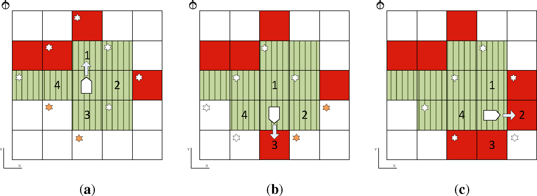
To ensure a correct mapping process, the exploration approach must ensure that every accessible cell is either visited or sensed. Existing algorithms move the robot to a location at which it can gather new information [2,3]. Selecting this location requires complex processing in a computer. To simplify the mapping process, the robot implements an optimized version of Trémaux’s Algorithm [22] in which the robot may only navigate to a neighbor cell. The neighbor cells are defined as the orthogonal ones in the matrix representation, i.e., the neighbors to the cell (i, j) are (i, j − 1), (i, j + 1), (i − 1, j), (i + 1, j). These cells will be the only ones that are considered in the next iteration when the robot moves. Hence, the robot’s movements are just 90-degree angle turns and linear movements equal to the length of a cell. The choice of the neighbor for the next iteration displacement is made using a clockwise priority. In our case, the first cell to visit will be the north one (i.e., (i, j − 1)) (see Figure 2a). The robot will visit this cell if it has uncharted neighbors and it is unoccupied; otherwise, the robot will choose, clockwise, the next neighbor of the current cell. In Figure 2a, neighbors 1 and 2 are discarded, because they do not have uncharted neighbors, so cell 3 is chosen. For the same reason, in Figure 2b, neighbor 2 is chosen. Finally, if the robot has no available neighbor to visit (Figure 2c), it will backtrack to a previous cell that meets the uncharted neighbor condition. This algorithm ensures that every cell of the map is either visited or sensed.
One important decision for implementing an Occupancy Grid Map is defining the cell’s size. Ideally, the smaller the size is, the more accurate the map will be. However, it will require more memory space and sensor accuracy. In our case, the objective is enabling the navigation of robots through the mapped zone. If the cells are smaller than the robot size, navigation planning will be more complex. In this proposal, a trade-off solution has been reached: the cell has been dimensioned as the minimum space where the robot fits and is able to turn around without crashing. Furthermore, it must be noted that a narrow cell-side width corridor may not be accessed. It depends on the alignment between the grid and this corridor. To ensure the mapping of a narrow corridor, it must be, at least, the size of the cell.
3.2. Sensors Structure
As introduced in Section 2, range finder sensors are suitable for our approach. To avoid interference with the localization system (see the next section), infrared sensors have been chosen to measure distances to obstacles. Infrared sensors measure distances by emitting infrared beams, which are reflected by the objects. The infrared beam is very narrow and directional, so defining the position of the detected obstacle is a simple task. The reflected beam is received by a position-sensitive photoelectric detector. This sensor uses a triangulation method considering the angle of deviation of the reflected infrared beam to measure the distance to the obstacle. As the infrared sensors measure the deviation angle of an object’s reflection, temperature and variation in the reflectivity of the object do not influence this measure. The output is an analog signal between 3.1 V and 0.3 V. The voltage output is digitized by an external ADC (analog-to-digital converter) before being driven to the FPGA board. The IRvoltage output can be modeled by an arctangent in order to obtain the distance. However, to avoid using the arctangent function, which takes more processing resources, and without losing accuracy, an experimentally obtained look-up-table has been used.
The linearity of the IR beams requires moving the sensor to scan an area. This movement may be done either by rotating the sensor or by displacing it. The IR sensors are fixed in the robot’s structure, so the sensing will be performed while the robot is moving. In this way, no additional motors are necessary for moving the sensors. The sensors have been positioned in the robot allowing, after the robot has moved from cell (i) to the next one (i + 1), all the neighbors of cell (i + 1) to be sensed.
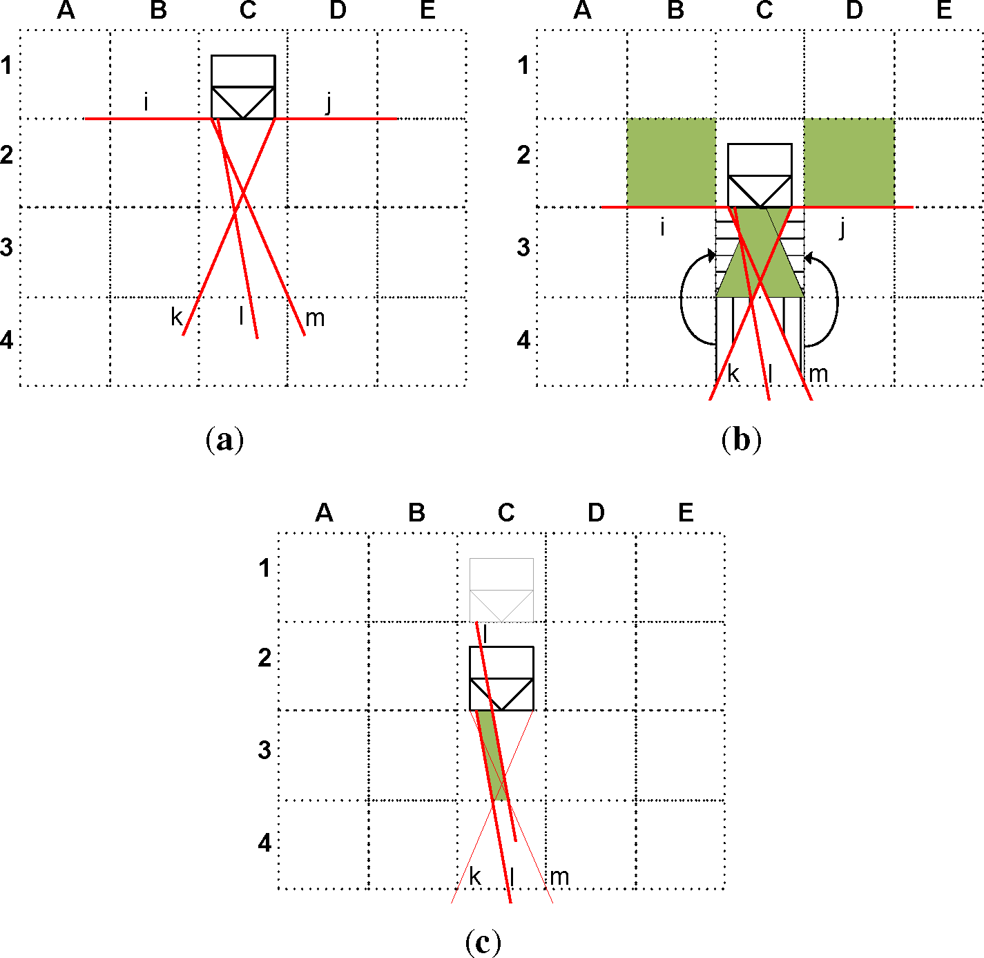
The disposition of the IR sensors is presented in Figure 3. This figure shows that after the transition from C1 to C2, cells B2, C3 and D2 have been sensed. Sensors i and j are placed at the sides of the robot and oriented orthogonally to the robot’s movement direction. When the robot moves from C1 to C2, these sensors cover cells B2 and D2 like a scanner. The cell at the front is more difficult to be completely sensed. When the robot moves from C1 to C2, sensors k and m scan the green area of C3 and the vertically marked area of C4 (see Figure 3b). The horizontally marked area of C3 is equivalent to that of C4 and was previously sensed in the transition from C0 to C1. However, a small triangle of C3 was not sensed by beams k and m. Figure 3c shows that this small triangle is scanned by beam l. These three beams, k, l and m, work like a snowplow truck. The angles of beams k and m are defined so each beam points to the opposite vertexes of the second cell to the front.
The disposition of the sensors and the robot motion ensure that all the cell’s surface is checked within the high accuracy range of the sensors. Considering the narrowness of the beams, the probability of not detecting an obstacle within sensor range is very low. An undetected obstacle would lead to the worst possible error in this scenario, defining an occupied cell as free. On the other hand, a wrong measurement of the sensor would define a free cell as occupied. The proposed solution promotes that any possible error falls into the second error category, which is not as hazardous as the first one for the robot.
3.3. Localization
The position of the robot is obtained using a system based on ultrasonic beacons, particularly, the method proposed in [16,17]. It measures the distances to three anchor points (ultrasound emitters) using the time of flight of the ultrasonic waves. The synchronization is based on radio frequency (RF) signals, required to know when the ultrasonic signals have been emitted. These ultrasound emitters are located on the ceiling of the room to be mapped. Trilateration using these three distances provides two possible solutions, but one of them is over the ceiling, so it can be discarded. The system obtains a mean error below 3.5 cm. However, this accuracy is only obtained if the robot is still.
The previous section presented that the beams detect obstacles while the robot is moving. Hence, it is important to know the robot’s exact position while moving to correctly place any detected object. The localization while moving is calculated using motor encoders, one per motor. These encoders provide pulses, corresponding to an angular distance. Therefore, knowing the radius of the robot’s wheel, it is possible to calculate the linear displacement. Finally, the robot calculates its current position by adding its previous ultrasound-obtained position and the distance obtained from the encoder information.
The main drawback of the encoder-based localization is its cumulative error, which obviously affects the mapping accuracy. For that reason, the robot needs to get its position using the ultrasonic-based localization system to avoid this cumulative error. This process is performed after two linear movements or after the linear movement following a rotation.
3.4. BOBMapping Algorithm
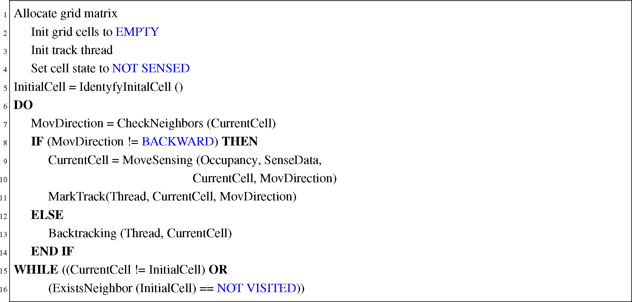
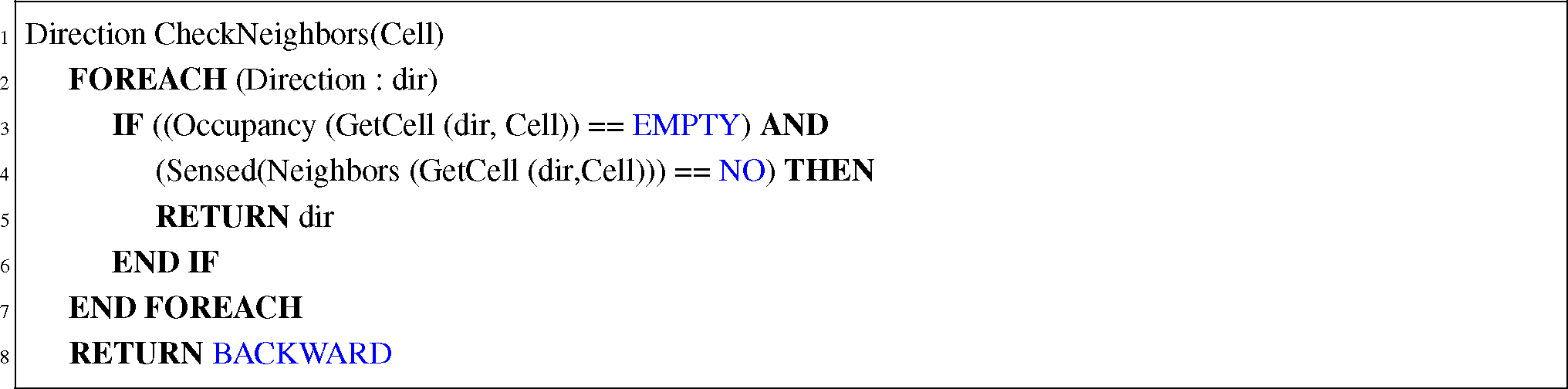
The proposed exploring method, presented in Section 3.1, ensures that every accessible cell is either visited or sensed. Hence, the algorithm will map all the available space (Code 1). Although the environment exploration algorithm does not restrict the initial cell election, the sensor structure requires the robot to be initially positioned in a cell whose frontal neighbor is unoccupied. This algorithm includes an optimization related to the decision of the neighbor to visit in the following iteration (Code 2). This optimization will make the robot omit those movements, leading to already known information (sensed cells), so the duration of the mapping process is optimized. The algorithm will finish on two conditions: (i) the robot returns to the initial cell, and it has no explorable neighbor; or (ii) every single cell of the grid has been sensed. However, if during any displacement, the robot checks a previously sensed cell, it changes its status depending on the new reading with one exception: if the new reading indicates that a cell that has been visited by the robot is occupied, this information will be discarded, because the cell is empty. We can assure that, because the robot passed through the cell without collision.
Section 3.2 described the disposition of the sensors and which cells were sensed in each step. For each cell in the grid, the algorithm stores four bits of data during the mapping process. The first of these bits represents the occupancy of the cell, being zero for a free cell. A second bit represents if the cell has been sensed or not. Therefore, if the cell is not sensed, the occupancy bit is ignored. Finally, the remaining two bits are used for backtracking. These two bits are used to codify the direction, from the four possible ones, that the robot took to reach that cell. This information is required in order to perform backtracking. Nevertheless, the final map will only record the occupancy information of each cell, requiring just one bit per cell.

The previous paragraph described the behavior of the algorithm in an ideal environment. However, in a real implementation, the algorithm must be robust enough to handle unexpected circumstances. Particularly, in this design, odometry may lead to inaccurate data. The slipping of wheels causes the robot to turn less than the planned angle or to move a shorter distance. Consequently, the detected obstacles may be placed in the wrong position. To handle these errors, the ultrasonic localization system is used. The position error is calculated, which is the difference between the expected position based on odometry and the position based on the ultrasound system. If it exceeds a threshold, a repositioning is carried out. The robot calculates the angle deviation between its position and the position it was supposed to be at, but in the previous cell. It moves backwards to the center of the previous cell and restarts the last step, sensing the neighbor cells again.
4. Experiments
This section presents experiments that have been performed with a real robot. A robot has been designed to test the algorithm in real situations. Experiments include accuracy testing of the infrared sensors and mapping generation of real environments.
4.1. Mobile Robot Architecture
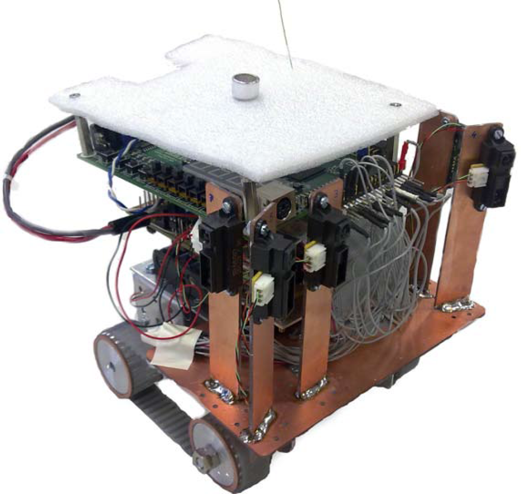
The implemented robot dimensions are 16 cm × 15 cm × 18 cm. The mobility of the robot is obtained using 2 DC motors (GHM-04 from Lynxmotion) with a 30:1 gearbox, and their speed is controlled with DPWM (digital pulse width modulation) signals. The motor shafts are attached to wheels that drive caterpillar tracks. The DC motors are also connected to optical encoders for odometry purposes (quadrature optical encoders E4P-100-079-DHTB).
An infrared sensor structure is placed at the front of the robot in a rigid piece that fixes the direction of each sensor. As was presented in Section 3.2, there are three forward-facing IR sensors and two other ones looking on both sides of the robot. The forward-facing infrared sensors are Sharp 2Y0A21, which provide an analog output proportional to the distance to the obstacle. The working range of these sensors is from 10 to 80 cm. The lateral IR sensors are Sharp 2D120X, which also provide an analog output and whose range is between 3 and 35 cm. The infrared sensor output is digitized with an ADC, so that a digital circuit, such as a microprocessor, can handle it. At the top of the robot, in its center, there is an ultrasonic receiver. This receiver is used by the localization system, which was explained in Section 3.3. The localization system also uses a radio-frequency receiver (FM-RRFQ2) in order to synchronize ultrasonic transmitters and receivers. Wireless communication between the robot and the computer is carried out thanks to an XBee module, which implements the ZigBee standard protocol.
All these elements are connected to an auxiliary board, which translates voltage levels to the FPGA working levels. This auxiliary board also includes a voltage regulator and a two-stage amplification and digitalization circuit connected to the ultrasound receivers. The controller of the robot has been implemented in an FPGA Xilinx Spartan3-1000 Starter board. The FPGA includes a 32-bit Microblaze embedded processor, which runs the proposed mapping algorithm detailed in Section 3.4. The processor is connected to several peripherals to perform auxiliary tasks, such as motor controlling, positioning, interfacing with the ADCs and wireless communication. Therefore, the FPGA allows one to design ad hoc hardware with a short design time, so it is suitable for prototyping. However, after testing, the proposed system can be implemented in a low cost digital signal processor (DSP) or microcontroller. Figure 4 shows a picture of the robot that has been designed and implemented.
Regarding the required hardware resources, the FPGA uses 3, 228 FlipFlops, 4, 581 4-input lookup tables (LUTs), three 18-bit multipliers and partially uses the internal 32 kB RAM and part of the 512 kB external RAM. Therefore, the proposed system fits in a low-cost FPGA.
On the other hand, software implementation needs 165 kB to implement the BOBMapping algorithm. The program also needs memory space in order to store the map, and this space is proportional to the grid size. As stated before, each cell requires four bits to be represented during the mapping process and one bit for map representation. In order to make it easier to index the array of bits, each row of the grid requires an integer number of bytes. For instance, if rows have 11 cells, 44 bits (5.5 bytes) are required to store the row during the mapping process, but six bytes are used. In the experiments, a grid map of 11 × 14 cells has been used, so 84 bytes have been used during the mapping process and 28 bytes have been used for map representation. The memory resources required by the algorithm and map representation would also fit in a low cost DSP or microcontroller, although a low-cost FPGA has been used for prototyping purposes.
4.2. Experiment’s Environment
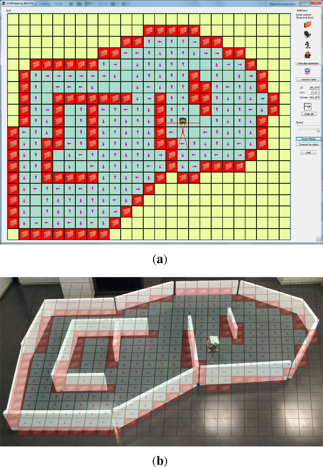
For real experiments, a laboratory room has been used. The obstacles have been simulated using expanded polystyrene barriers. The implemented robot was used for these experiments. As stated before, the grid map used in these experiments has 11 × 14 cells. Taking into account the size of the robot, the cell side length has been set to 22 cm. Therefore, the real experiments were performed in a 242 × 308 cm area.
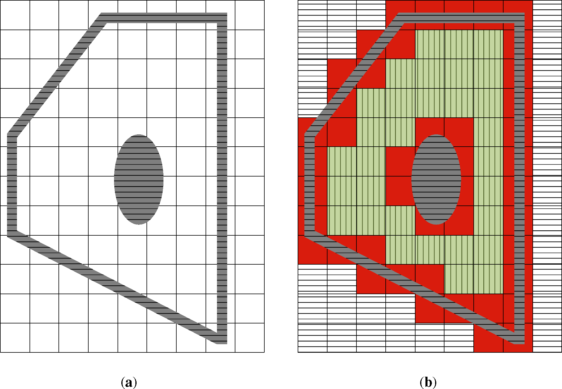
An application has been developed to monitor the mapping process accomplished by the robot (Figure 5a). This application implements a GUI (graphic user interface) to represent the navigation steps and also shows the cells that have been sensed by the robot. The application does not interact with the robot, but is just a listener, which receives information from the robot through the ZigBee communication modules; so, the robot remains completely autonomous.
Figure 5b is the picture of the real environment explored in this experiment. The result of the monitoring application has been superimposed on the picture.
4.3. Experimental Results
The proposed algorithm trusts in the information of the infrared sensors and the localization system to set the occupancy state of a cell. The localization system was presented in [17] and provides an accuracy of 3.3 cm. The accuracy of the distances to obstacles is a key component in this proposal, because it does not use cell occupancy probabilities, but binary states: empty or occupied. Therefore, experiments have been performed to test the accuracy of the infrared sensors, both front and lateral.
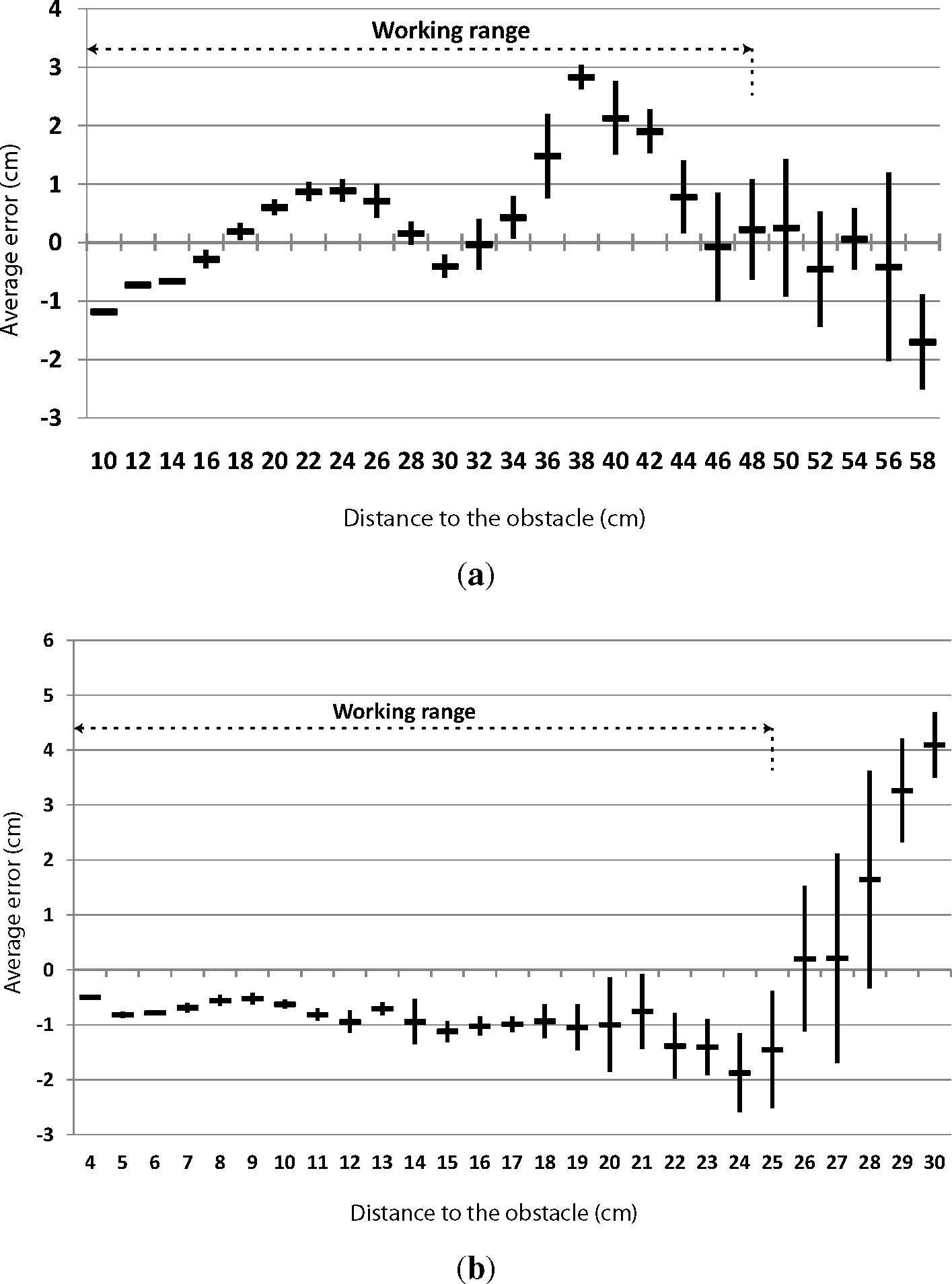
An obstacle has been placed at different distances to the sensors. When testing the front sensors, the obstacle has been placed every 2 cm between 10 to 58 cm. Regarding the lateral sensors, the obstacle has been placed every 1 cm between four to 30 cm. Figure 6a,b shows the results of the experiments performed with the front and lateral sensors, respectively. The figures show the average error with its standard deviation. As can be seen, the accuracy of the obstacle distance estimation decreases as the obstacle is farther away.
The required range of the IR sensors is set by the cell side length of the map, 22 cm in these experiments, and the geometrical considerations explained in Section 3.2. The front IR sensors are used to detect obstacles from 10 to 48 cm. The minimum distance of obstacle detection by the Sharp 2D120X IR sensor is 10 cm. The maximum distance required by the k and m sensors (see Figure 3) is 48 cm, when the cell side length is 22 cm and the robot is centered in its current cell. As Figure 6a shows, the maximum average error between 10 and 48 cm is below 3 cm; so, the obstacle distance estimation is quite accurate. The lateral sensors are used to detect obstacles from four to 25 cm. The minimum distance of obstacle detection by the Sharp 2Y0A21 IR sensor is 4 cm. Additionally, 25 cm is the maximum distance required to sense the neighbor lateral cell, taking into account that the cell side length is 22 cm, and the robot is centered in its current cell. Taking this range (four to 25 cm), the maximum average error of the lateral sensors is 2 cm; so, the lateral sensors are also quite accurate.
Once the infrared sensors have been tested, mapping experiments with the robot have been performed, as Figure 5 shows.
In the mapping experiments, 10 space configurations have been set, and the robot has been ordered to map its environment. Some of the configurations are closed space maps, where all the space is limited by barriers. Besides, open space configurations have been mapped, where the limit of the space is limited by the grid size. Table 1 shows the results of the experiment. As explained in Section 3.4, the robot can re-sense a previously sensed cell when the robot is moving, so this information is detailed in the table. The table also shows the accuracy of the mapping and the number of cells that the robot has to move in order to map the environment, as well as the number of the robot’s turns during this process.
It is important to notice that all the errors in the mapping process have arisen in boundaries between empty and occupied cells, especially when an obstacle was in the boundary between cells. The previously described re-sensing technique allows one to reduce the number of errors in the mapping process, while it does not increment the mapping time. In these experiments, 20 errors arose while mapping, but using the re-sensing process, the errors dropped to six. As was described in Section 3.2, the mapping process minimizes the possibility of classifying an occupied cell as empty; all the errors in Table 1 are empty cells mapped as occupied cells. Therefore, a moving robot will not bump into an obstacle due to mapping errors.
Finally, Table 1 shows the length of the path, given in the number of cells, covered by the robot and the number of turns. The results show that, on average, the robot has to visit an average of 68% of the cells to complete the final map, including backtrack movements. This large percentage is related to the low sensing range. The required increase of sensor accuracy slows the mapping process compared to solutions with wider the sensing range.
The average success rate of the mapping experiments is 99.42%, so the generated maps are very similar to the real environments. Therefore, these maps are suitable to be used in the unassisted navigation of indoor robots.
5. Discussion
We presented in Section 2 the current state-of-the-art related to map building. At this point of the paper, a comparison with similar approaches is required. This section will focus on two main points: the cost of the system and the mapping algorithm.
Different works have included low-cost requirements in their design. Magnenat et al. [23] creates occupancy-grid maps using an infrared rotating sensor. Although the full price of the robot is not reported, just the rotating sensor unit costs $390. Gifford et al. [24] created an autonomous mapping robot using IR sensors. The reported price of each unit is $1, 250. The cost of the system presented in this paper is $550, including the price of the two FPGAs required (one for the robot and the other for the ultrasonic beacon system). Each of these FPGAs costs around $130. However, cheaper FPGAs would be also valid for the project. Furthermore, the emitting beacons can be controlled using a microcontroller, which is cheaper than an FPGA, as all the localization processing is performed in the receiver node.
The space exploration algorithm is highly dependent on sensor range and the use of the already explored map. When the robot is able to sense a multiple cell radius area and use the already explored map, choosing the next position to perform an unknown cell search falls into the following approaches. In [25], the Next-Best-View strategy is used: the best candidate for a new search is the position that will allow for the gathering of more information. The Distance Transform is used in [26]; in this algorithm, the best candidate is the nearest unknown position. Finally, the algorithm in [27] considers for every candidate the possibility of gathering information and the distance to the current position. When the already explored map is not considered, there are different proposals for map exploration: in [28] different paths (Seedspreader, Concentric, FigureEight, Random, Triangle and Star) are considered and evaluated. Two wall-following strategies are presented in [29], and the results of using random paths are discussed in [30].
In the BOBMapping approach, during the forward exploration stage, the algorithm is based on Trémaux’s Algorithm. As presented before, three cells are completely sensed for each position. This information is included in Trémaux’s Algorithm to select the next cell to be visited. Considering the low sensing range, the robot’s final mapping path is very similar to Trémaux’s base solution. Besides, our approach uses the information of the explored map when it backtracks, reducing the traveled distance.
To the best of the authors knowledge, the BOBMapping approach is one of the cheapest mapping algorithms. The proposed algorithm is also one of the slowest solutions compared to [25–27]. However, it is important to notice that the mapping process is accomplished only once, so the mapping time should not be critical.
6. Conclusions
This paper describes BOBMapping, which is a mapping approach designed to be used by low-cost robots. The presented proposal is based on simplified Occupancy Grid Mapping systems, optimized for low-cost devices. The cells of the maps are represented by a binary state, completely empty or partially/fully occupied, so there are no probabilities in the state of the cell. This way, the required resources (memory and algorithm complexity) of the system are reduced. This design is motivated by the fact that the robot has the same size as the cell, and it is holonomic. This paper proposes an optimized geometrical distribution of linear IR sensors to fully scan the area of several cells in one iteration.
The algorithm for space exploration is based on Trémaux’s Algorithm. In this approach, the robot explores its orthogonal neighbor cells and stores the required information to track its route. When the robot reaches a cell where all its neighbors do not have any un-sensed cell, it backtracks with the navigation information that has been previously stored. The exploration approach shows lower performance than mapping algorithms, which use already explored information to decide the mapping path. This difference is based on our shorter, although more accurate, sensing range. However, the proposed solution improves those mapping approaches that ignore previously explored space.
The implementation has been tested with a real robot that uses IR sensors for detecting obstacles. The localization system provides an accuracy of 3.3 cm. Accuracy experiments of the infrared sensors have been performed showing that the error remains under 3 cm in all the measurement ranges. Besides, mapping experiments have been accomplished with a success rate of 99.42% in real environments. Hence, the BOBMapping algorithm has shown its reliability in creating Occupancy Grid Maps.
Acknowledgments
This work has been supported by the Spanish Ministerio de Ciencia e Innovación under project TEC2009-09871.
Conflicts of Interest
The authors declare no conflict of interest.
References
- Chen, C.; Cheng, Y. Research on Map Building by Mobile Robots, Proceedings of the Second International Symposium on Intelligent Information Technology Application (IITA ’08), Shanghai, China, 20–22 December 2008; 2, pp. 673–677.
- Yamauchi, B. A Frontier-Based Approach for Autonomous Exploration, Proceedings of the 1997 IEEE International Symposium on Computational Intelligence in Robotics and Automation (CIRA’97), Monterey, CA, USA, 10–11 July 1997; pp. 146–151.
- Stachniss, C. Robotic Mapping and Exploration; Springer: Berlin, Germany, 2009. [Google Scholar]
- Vaughan, R.; Stoy, K.; Sukhatme, G.; Mataric, M. LOST: Localization-space trails for robot teams. IEEE Trans. Robot. Autom. 2002, 18, 796–812. [Google Scholar]
- Arleo, A.; del R. Millan, J.; Floreano, D. Efficient learning of variable-resolution cognitive maps for autonomous indoor navigation. IEEE Trans. Robot. Autom. 1999, 15, 990–1000. [Google Scholar]
- Cuesta, F.; Ollero, A. Chapter 4 Intelligent Control of Mobile Robots with Fuzzy Perception. In Intelligent Mobile Robot Navigation; Springer: Berlin, Germany, 2005; pp. 79–122. [Google Scholar]
- Nagla, K.; Uddin, M.; Singh, D. Improved occupancy grid mapping in specular environment. Robot. Auton. Syst. 2012, 60, 1245–1252. [Google Scholar]
- Lopez-Sanchez, M.; Esteva, F.; Lopez de Mantaras, R.; Sierra, C.; Amat, J. Map generation by cooperative low-cost robots in structured unknown environments. Auton. Robot. 1998, 5, 53–61. [Google Scholar]
- Bräunl, T. Embedded Robotics: Mobile Robot Design and Applications With Embedded Systems; Springer-Verlag-Berlin: Heidelberg, Germany, 2008. [Google Scholar]
- Anousaki, G.; Kyriakopoulos, K. Simultaneous localization and map building of skid-steered robots. IEEE Robot. Autom. Mag. 2007, 14, 79–89. [Google Scholar]
- Castellanos, J.A.; Tardós, J.D. Mobile Robot Localization and Map Building a Multisensor Fusion Approach; Springer: Berlin, Germany, 2000. [Google Scholar]
- Vázquez-Martín, R.; Nunez, P.; Bandera, A. LESS-mapping: Online environment segmentation based on spectral mapping. Robot. Auton. Syst. 2012, 60, 41–54. [Google Scholar]
- Kim, G.; Kwak, N.; Lee, B. Low Cost Active Range Sensing Using Halogen Sheet-of-Light for Occupancy Grid Map Building, Proceedings of the 2005 IEEE/RSJ International Conference on Intelligent Robots and Systems (IROS 2005), Edmonton, AB, Canada, 2–6 August 2005; pp. 1612–1617.
- Choi, Y.H.; Oh, S.Y. Map building through pseudo dense scan matching using visual sonar data. Auton. Robot. 2007, 23, 293–304. [Google Scholar]
- Umbarkar, A.; Subramanian, V.; Doboli, A. Low-cost sound-based localization using programmable mixed-signal systems-on-chip. Microelectron. J 2011, 42, 382–395. [Google Scholar]
- Sanchez, A.; Elvira, S.; de Castro, A.; Glez-de Rivera, G.; Ribalda, R.; Garrido, J. Low Cost Indoor Ultrasonic Positioning Implemented in FPGA, Proceedings of the 35th Annual Conference of IEEE Industrial Electronics (IECON ’09), Porto, Portugal, 3–6 November 2009; pp. 2709–2714.
- Sanchez, A.; de Castro, A.; Glez-de-Rivera, G.; Elvira, S.; Garrido, J. Autonomous indoor ultrasonic positioning system based on a low-cost conditioning circuit. Measurement 2012, 45, 276–283. [Google Scholar]
- Birk, A.; Carpin, S. Merging occupancy grid maps from multiple robots. IEEE Proc. 2006, 94, 1384–1397. [Google Scholar]
- Elfes, A. Using occupancy grids for mobile robot perception and navigation. Computer 1989, 22, 46–57. [Google Scholar]
- Pala, M.; Osati Eraghi, N.; López-Colino, F.; Sanchez, A.; de Castro, A.; Garrido, J. HCTNav: A path planning algorithm for low-cost autonomous robot navigation in indoor environments. ISPRS Int. J. Geo-Inf. 2013, 2, 729–748. [Google Scholar]
- Quigley, M.; Gerkey, B.; Conley, K.; Faust, J.; Foote, T.; Leibs, J.; Berger, E.; Wheeler, R.; Ng, A. ROS: An Open-Source Robot Operating System, Proceedings of the Open-Source Software Workshop of the International Conference on Robotics and Automation (ICRA), Kobe, Japan, 12–17 May 2009.
- Even, S. Graph Algorithms; Cambridge University Press: Cambridge, UK, 2011. [Google Scholar]
- Magnenat, S.; Longchamp, V.; Bonani, M.; Retornaz, P.; Germano, P.; Bleuler, H.; Mondada, F. Affordable SLAM through the Co-Design of Hardware and Methodology, Proceedings of the 2010 IEEE International Conference on Robotics and Automation (ICRA), Anchorage, AK, USA, 3–7 May 2010; pp. 5395–5401.
- Gifford, C.; Webb, R.; Bley, J.; Leung, D.; Calnon, M.; Makarewicz, J.; Banz, B.; Agah, A. Low-Cost Multi-Robot Exploration and Mapping, Proceedings of the IEEE International Conference on Technologies for Practical Robot Applications (TePRA 2008), Woburn, MA, USA, 23–24 April 2008; pp. 74–79.
- Gonzalez-Banos, H.H.; Latombe, J.C. Navigation strategies for exploring indoor environments. Int. J. Robot. Res. 2002, 21, 829–848. [Google Scholar]
- Taylor, T.; Geva, S.; Boles, W. Directed Exploration Using a Modified Distance Transform, Proceedings of the 2005 Digital Image Computing: Techniques and Applications (DICTA ’05), Cairns, Australia, 6–8 December 2005; pp. 53–53.
- Amigoni, F.; Caglioti, V. An information-based exploration strategy for environment mapping with mobile robots. Robot. Auton. Syst. 2010, 58, 684–699. [Google Scholar]
- Sim, R.; Dudek, G. Effective Exploration Strategies for the Construction of Visual Maps, Proceedings of the 2003 IEEE/RSJ International Conference on Intelligent Robots and Systems (IROS 2003), Las Vegas, NV, USA, 27–31 October 2003; 4, pp. 3224–3231.
- Lee, D.; Recce, M. Quantitative evaluation of the exploration strategies of a mobile robot. Int. J. Robot. Res. 1997, 16, 413–447. [Google Scholar]
- Freda, L.; Oriolo, G. Frontier-Based Probabilistic Strategies for Sensor-Based Exploration, Proceedings of the 2005 IEEE International Conference on Robotics and Automation (ICRA 2005), Barcelona, Spain, 18–22 April 2005; pp. 3881–3887.


| Map | Number of Cells in the Configuration | Re-Sensed Cells During Mapping | Empty Cells Sensed as Occupied | Occupied Cells Sensed as Empty | Success Rate | Length Path (Number of Cells) | Number of Turns |
|---|---|---|---|---|---|---|---|
| 1 | 55 | 1 | 0 | 0 | 100% | 30 | 19 |
| 2 | 151 | 0 | 0 | 0 | 100% | 108 | 37 |
| 3 | 148 | 0 | 3 | 0 | 97.97% | 117 | 4 |
| 4 | 317 | 0 | 0 | 0 | 100% | 243 | 92 |
| 5 | 51 | 2 | 0 | 0 | 100% | 29 | 11 |
| 6 | 80 | 2 | 0 | 0 | 100% | 44 | 19 |
| 7 | 51 | 2 | 0 | 0 | 100% | 25 | 8 |
| 8 | 85 | 1 | 1 | 0 | 98.82% | 57 | 30 |
| 9 | 76 | 5 | 2 | 0 | 97.37% | 44 | 22 |
| 10 | 55 | 1 | 0 | 0 | 100% | 36 | 29 |
| Total | 1, 069 | 14 | 6 | 0 | 99.42% | 732 | 271 |
© 2013 by the authors; licensee MDPI, Basel, Switzerland This article is an open access article distributed under the terms and conditions of the Creative Commons Attribution license (http://creativecommons.org/licenses/by/3.0/).
Share and Cite
Gonzalez-Arjona, D.; Sanchez, A.; López-Colino, F.; De Castro, A.; Garrido, J. Simplified Occupancy Grid Indoor Mapping Optimized for Low-Cost Robots. ISPRS Int. J. Geo-Inf. 2013, 2, 959-977. https://doi.org/10.3390/ijgi2040959
Gonzalez-Arjona D, Sanchez A, López-Colino F, De Castro A, Garrido J. Simplified Occupancy Grid Indoor Mapping Optimized for Low-Cost Robots. ISPRS International Journal of Geo-Information. 2013; 2(4):959-977. https://doi.org/10.3390/ijgi2040959
Chicago/Turabian StyleGonzalez-Arjona, David, Alberto Sanchez, Fernando López-Colino, Angel De Castro, and Javier Garrido. 2013. "Simplified Occupancy Grid Indoor Mapping Optimized for Low-Cost Robots" ISPRS International Journal of Geo-Information 2, no. 4: 959-977. https://doi.org/10.3390/ijgi2040959
APA StyleGonzalez-Arjona, D., Sanchez, A., López-Colino, F., De Castro, A., & Garrido, J. (2013). Simplified Occupancy Grid Indoor Mapping Optimized for Low-Cost Robots. ISPRS International Journal of Geo-Information, 2(4), 959-977. https://doi.org/10.3390/ijgi2040959