Georeferenced Point Clouds: A Survey of Features and Point Cloud Management


Abstract
: This paper presents a survey of georeferenced point clouds. Concentration is, on the one hand, put on features, which originate in the measurement process themselves, and features derived by processing the point cloud. On the other hand, approaches for the processing of georeferenced point clouds are reviewed. This includes the data structures, but also spatial processing concepts. We suggest a categorization of features into levels that reflect the amount of processing. Point clouds are found across many disciplines, which is reflected in the versatility of the literature suggesting specific features.1. Introduction and Motivation
With the increase of advanced electromagnetic imaging in surveying and geoinformatics, massive datasets are generated. That data are points located in three dimensional space and exhibit the characteristics of the applied measurement method, which can be active or passive and record different properties of the electromagnetic waves (spectral measurement, time of detection, etc.). Further, algorithms are applied to the data to compute higher order attributes (features), which enhance the description of these points. Since the resulting datasets usually contain billions of points and the computational algorithms are often complex to execute, appropriate management of these datasets is required. This is generally highly dependent on the applications for which data are used. The paper gives an overview of different data handling approaches, independent of the acquisition method and the application. Spatial access, extending attributes and processing concepts, including the use of secondary storage next to random access memory, are considered.
In this article, a point cloud is defined as a set of points, Pi, i = 1, …, n, embedded in three-dimensional Cartesian space. The term “cloud” reflects the unorganized nature of the set and its spatial coherence, however, with an unsharp boundary. A georeferenced point cloud is given in an Earth-fixed coordinate system, e.g., an Earth-centered system, like WGS84 (World Geodetic System, 1984), or in a map projection with a specified reference ellipsoid, e.g., UTM (Universal Transverse Mercator). Each point, Pi has three coordinates, (xi, yi, zi)⊤ ∈ R3, but may have additional attributes, aj,i, with j = 1, …, mi, the number of attributes of point i. An attribute, aj, may be, e.g., one of nx, ny, nz, σz, r, g, b, nIR, resembling normal vector components, elevation accuracy and “color” in four spectral bands. Defining a normal vector requires that the points are sampled from piecewise continuous surfaces, in which case, a tangent plane exists, in general, for each point. This tangent plane can be estimated from the points, and the normal vector is the direction perpendicular to it. There may be conditions imposed on the attributes, e.g., that the square sum of the normal vector components equals one. A unit vector of a length of one is appropriate, because the normal vector shall only denote the direction perpendicular to the tangent plane in the point, whereas the length of the vector has no meaning. Each point, Pi is therefore a vector, (xi, yi, zi, a1,i, …, ami,i)⊤, of a dimension of 3 + mi, with a fixed meaning for the first three components, i.e., the point coordinates. The other components of the vector may have a different meaning for different points in the cloud. If a point cloud contains points from two or more sources, for example, from different acquisition campaigns, platforms or measurement devices, each set coming from one source can have its specific set of features, although all points are in the same coordinate system.
Point clouds describing topography can be generated from laser scanning, image correlation, radargrammetry, SAR (Synthetic Aperture Radar) tomography, time of flight cameras (ToF cameras) and Multi-beam Echo Sounding (MBES). There is no convention to define the scale of a point cloud, as, e.g., an image may have, but rather, a typical sampling distance of the points over the topographic area of interest may be defined. Depending on the acquisition method and platform, this sampling distance may be as small as a few centimeters, e.g., from terrestrial laser scanning, but also as large as several hundreds of meters, e.g., the point clouds acquired by satellite laser altimetry. Aerial data acquisition often leads to clouds with billions of points. Topographic point clouds may cover larger areas, ranging from some tens of meters to an entire planet. As an example, the City of Vienna, with an area of 400 km2, was scanned with a density of 20 points per m2, resulting in 10 billion points [1], including a few additional features for each point. In Mølhave et al. [2], the processing of 26 billion points (x, y, z) for terrain model generation is described. Li et al. [3] reports the processing of 70 million points, with the feature vector containing more than 100 elements. Thus, suitable spatial data structures for point clouds are required for accessing, as well as local algorithms for processing, the point data.
Georeferenced point clouds are models of reality, related to a specific place (as given by their coordinates and the specification of the used coordinate system (We refer to Altamimi et al. [4] in which the realization of a reference system through fixed points (the reference frame) is explained. In their case, the system is the current International Terrestrial Reference System (ITRS).) and specific time (as given by its acquisition time). Thus, point clouds cannot only be used to visualize a scene (e.g., [5]), but also to infer quantitative information. As an example, distances between identified points can be measured to obtain the height of an underpass, or to measure the length of a fault line. Going one step further into automated analysis, including scene classification and geometric modeling, also, statistical information as the distribution of slope angles in a catchment may be derived from the points by analyzing their normal vectors. Of course, in this example, only points belonging to the terrain surface may be investigated, and the normal vector feature has to be computed beforehand.
Point clouds used in reverse engineering and geometric modeling [6] are often acquired by active triangulation (triangulating laser scanners) or coordinate measurement machines (CMM). The scene typically shows one object that needs to be modeled. Points from the background or other objects are deleted before further analysis. Modeling is often performed with free-form surfaces. In comparison, geo-referenced point clouds often carry the need for more semantic information in order to become useful, as multiple objects of different classes may be within the scene. In robotics, the term, point cloud, is sometimes used to refer to a set of points covering an object. The term “feature” of the the point cloud is also used to describe the property of the entire point set, i.e., an object of a particular class. Those “features” are computed by estimating the parameters of the entire set [7] (e.g., extent, shape fitting) or by identifying it.
Computing features of point sets is also found in object-based point cloud analysis [8,9], which has the concept of first summarizing homogeneous, spatially connected subsets of the points (i.e., segmentation) and, then, using this aggregated information for classification. In contrast, the current paper is focused on features of individual points.
In the context of SDI (Spatial Data Infrastructure), the formal description and distribution of geo-data is a topic. Retrieving point clouds from a repository is presented in Crosby et al. [10].
The contribution of this article is to: (i) give an overview of the features used in the processing of georeferenced point clouds; (ii) categorize the features; and iii) provide an overview of data structures and point cloud management. In the discussion, we also argue for maintaining the point cloud as the source data, rather than considering one surface model composed of planar or curved faces as the scene representation for all applications (see, also [5]).
The paper is organized as follows. Section 2 recapitulates the key facts of point cloud acquisition methods and summarizes the features as suggested in the literature. Next, in Section 3, an overview of the data structures used for large point clouds in persistent form, as well as during processing is given. In Section 4, we propose the sorting of features into categories and further discuss point cloud processing.
2. State-of-the-Art: Point Clouds and Features
2.1. Acquisition of Point Clouds
The measurement methods for obtaining point clouds are described from the perspective of what is being measured for each point, thus feature-oriented.
The term, LiDAR, stands for “Light Detection And Ranging”, but Measures [11] suggested to expand the acronym to “Laser Identification, Detection, Analysis and Ranging”, which indicates that more than range can be measured with LiDAR. A signal, either pulsed or continuously modulated, is emitted, and the time delay to detection of its echo is measured. This is, via the speed of light, transformed to the (two-way) distance from the sensor to the object and back to the detector. The emission direction is measured in the sensor coordinate system. Together with the exterior orientation of the platform (mobile or static), the location of the backscatter can be computed in the global coordinate system, thus providing the three coordinates (x, y, z)⊤ via direct georeferencing [12]. In discrete return laser scanning, also a measure of the backscatter strength is often provided as the digital number (DN). As the physical meaning of this measure is often not provided, it remains unclear if this refers to the peak amplitude or the energy of the entire echo and if it is linearly scaled. A method for relative calibration is given in Höfle and Pfeifer [13]. This backscatter strength can be normalized by range, possibly by incidence angle and, sometimes, also by reference values [14].
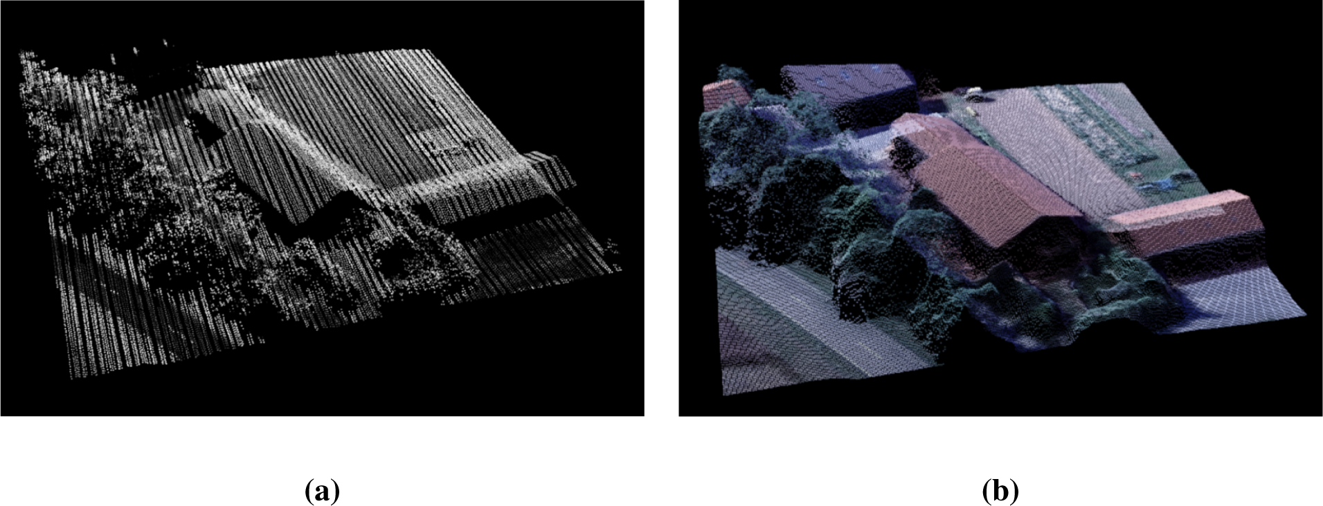
In full waveform laser scanning, the shape of the emitted pulse and the received echo are recorded, typically with a sampling interval on the order of one nano second (ns). This allows, on the one hand, rigorous radiometric calibration [15], and on the other hand, it provides additional measurements derived from the shape of the backscattered echo. The “radiometric” waveform parameters are the backscattering cross section (normalized to the footprint area) the backscattering coefficient and (normalized further by the angle of incidence and assuming Lambertian scattering) the diffuse reflectance. These values refer to the wavelength of the laser in use. The “geometric” waveform parameter is the echo width, which can be retrieved from the sampled echo waveform, typically the full width at half maximum (FWHM). Alternatively, it can be extracted from waveform modeling, e.g., by Gaussians or other basis functions [16]. Furthermore, other shape parameters, e.g., skewness, were suggested [17]. The radiometric values are unit-less, whereas the geometric values are either specified in length (m) or time (ns). The geometric waveform parameters depend not only on the object, but also on the shape of the emitted waveform. The differential cross section (e.g., [18]), which is obtained by deconvolving the echo waveform with the emitted waveform, only depends on the object and provides additional quantities, independent of mission parameters. For large footprint systems, e.g., ICESat (Ice, Cloud, and land Elevation Satellite), a comprehensive list describing waveform parameters is given by Duong [19]. An example showing the point cloud with the recorded full waveform amplitude is given in Figure 1a.
Mapping with images is singular, in the sense that points (x, y, z)⊤ of the 3D environment are mapped to a 2D image. Three-dimensional reconstruction is typically enabled by using more than one image of the same object. The measurements are, in comparison to laser scanners, not the coordinates of where the light was reflected, but the brightness (amount of light reflected) at that point as “seen” by the camera [20]. The location of the measurement is prescribed by the layout of the sensor pixels. Therefore, points at color or gray value differences (texture) can be identified. Together with the exterior orientation of the images, measured directly or derived by bundle block adjustment, the ray, which is mapping the point from object space to image space, is reconstructed. Rays of corresponding points across multiple images intersect in the object point (forward intersection). This forward intersection is overdetermined and, thus, an accuracy feature can be derived. This measure becomes more reliable with the number of rays used for intersection. The recorded color is a measurement, as well, and, thus, can become a feature of the point. Radiometric calibration can be performed for images of aerial photogrammetric cameras [21]. This typically supplies three or four bands (red, green, blue, near infrared, relating to the properties of the filters for separating the spectral bands), a measurement of the radiance at the sensor and, with further processing, an estimation of object radiance. The recorded or computed values all depend on one fundamental object point property, which is the Bi-directional Reflectance Distribution Function (BRDF, [22]). Point clouds are obtained by dense matching of image pairs (or more images), e.g., [23]. An example showing a point cloud from semi-global image matching with the recorded color is given in Figure 1b. The georeferencing of point clouds obtained by image matching is supplied either indirectly by ground control points (GCPs, [24]), directly by “direct geo-referencing” [12,25] or by “integrated geo-referencing”, exploiting control points and direct observations of the sensor’s exterior orientation [26]. The quality of different approaches is further investigated in Heipke et al. [27].
In the microwave domain of the electromagnetic spectrum, synthetic aperture radar (SAR) is used for imaging the Earth’s surface. Similar to photographic imaging, this map is singular, but it provides different measurements. Over the grid of the azimuth (along the flying direction) and range (across the flying direction), the complex backscatter strength, i.e., amplitude and phase, are recorded. SAR is side looking and, therefore, results in reduced visibility of surfaces not oriented towards the sensor, especially in comparison to airborne laser scanning and photographic imaging. A point cloud can be obtained from SAR by using a pair of images with a larger base-line and the identification of corresponding points in the amplitude image, i.e., radargrammetry [28,29]. In this case, the reflection strength is an additional measurement and becomes a point feature, as is the intersection quality in the case of overdetermination. Alternatively, tomographic SAR can be used to build a virtual aperture in the z direction and, thus, resolve the third dimension [30]. This provides the reflection strength, but also a coherence measure for each point.
Echo sounding can provide point clouds, as well, which need, like laser scanning, direct georeferencing for transforming the measurements from the sensor coordinate system into an Earth-fixed coordinate system. Different wavelengths are used, and dual wavelength systems are common, with larger wave lengths allowing the penetration of soft ground, e.g., mud vs. solid rock. The reflection strength may also be recorded and, thus, enrich the feature vector [31]. Point cloud processing of large MBES (Multi-beam Echo Sounding) datasets is described, e.g., in Arge et al. [32]. The case of MBES point clouds will not be discussed further.
In recent years, the availability of high frame rate 3D cameras, like ToF cameras and Kinect, have led to an increase in interest in point cloud data handling and processing. However, due to their restricted range (typically around 0.5 m to 5 m) and limitations in the outdoor usage, the literature on georeferenced point clouds from those 3D cameras is scarce [33].
2.2. Features of Point Clouds
In this section, we review the use of features, ranging from “color” to local neighborhood descriptions. In comparison to Section 2.1, the selection of features is driven from an application point of view rather than based on technical considerations related to measurement.
Color is a feature of a point, which is often used in display, segmentation and classification. Wand et al. [34] demonstrate the editing of huge (more than 2 × 10⁹ points) point clouds that contain not only the point position and RGB color, but also the normal vector and sample space information. Lichti [35], for example, suggested using red, green, blue and near infrared for the classification of point clouds. Color is the original measurement in cameras, but typically, these values are not calibrated.
By calibration, the original measurements may become improved features of the point, relating rather to object space and depending less on the data acquisition mission. Briese et al. [36] presented laser scanning point clouds acquired at three wavelengths, which are absolutely calibrated. Höfle et al. [37] use a calibrated reflectance for classification of water surfaces. With LiDAR, also, full waveform features can be exploited for the classification of vegetation, land cover and urban scenes, like the waveform width, number of echoes and backscatter coefficient, e.g., [38–41]. Backscatter coefficient and echo width, for example, are features that are directly measured or computed from and for each single point. For object reflectivity, a scattering model needs to be assumed, typically Lambertian scattering, which requires a normal vector and, therefore, a local surface model.
Additional information can be derived for each point, if its neighborhood is analyzed. Li et al. [3] use point clouds generated from image blocks by Structure from Motion (SfM). Their aim is to find the correspondence between a given image and a worldwide point cloud, which covered some thousand locations around the world. The feature used next to the point position is the SIFT (Scale Invariant Feature Transform) descriptor [42] from one or multiple images used for matching and reconstructing that particular point. The SIFT descriptor has a dimension of 128 and does not directly encode color, but, rather, gradient direction in the vicinity of the (image) point. It is rotation and scale invariant, but computed in the original image and, therefore, not invariant to (large) changes of the view point. Neighborhood is, in this case, derived from the image space, but can also be defined in object space. An example for the latter is intensity density, as suggested by Clode and Rottensteiner [43], which measures the portion of points in a neighborhood for which the feature “intensity” is above a certain threshold. Here, the neighborhood is used to get smoothed results, which are then used in classification. Similarly, point density is used in Brzank et al. [44] to classify coastal areas and water surfaces. Hammoudi et al. [45] project the 3D points vertically to the horizontal grid and use the resulting point density in the “accumulation map” [45,46] to segment vertical structures in urban areas.
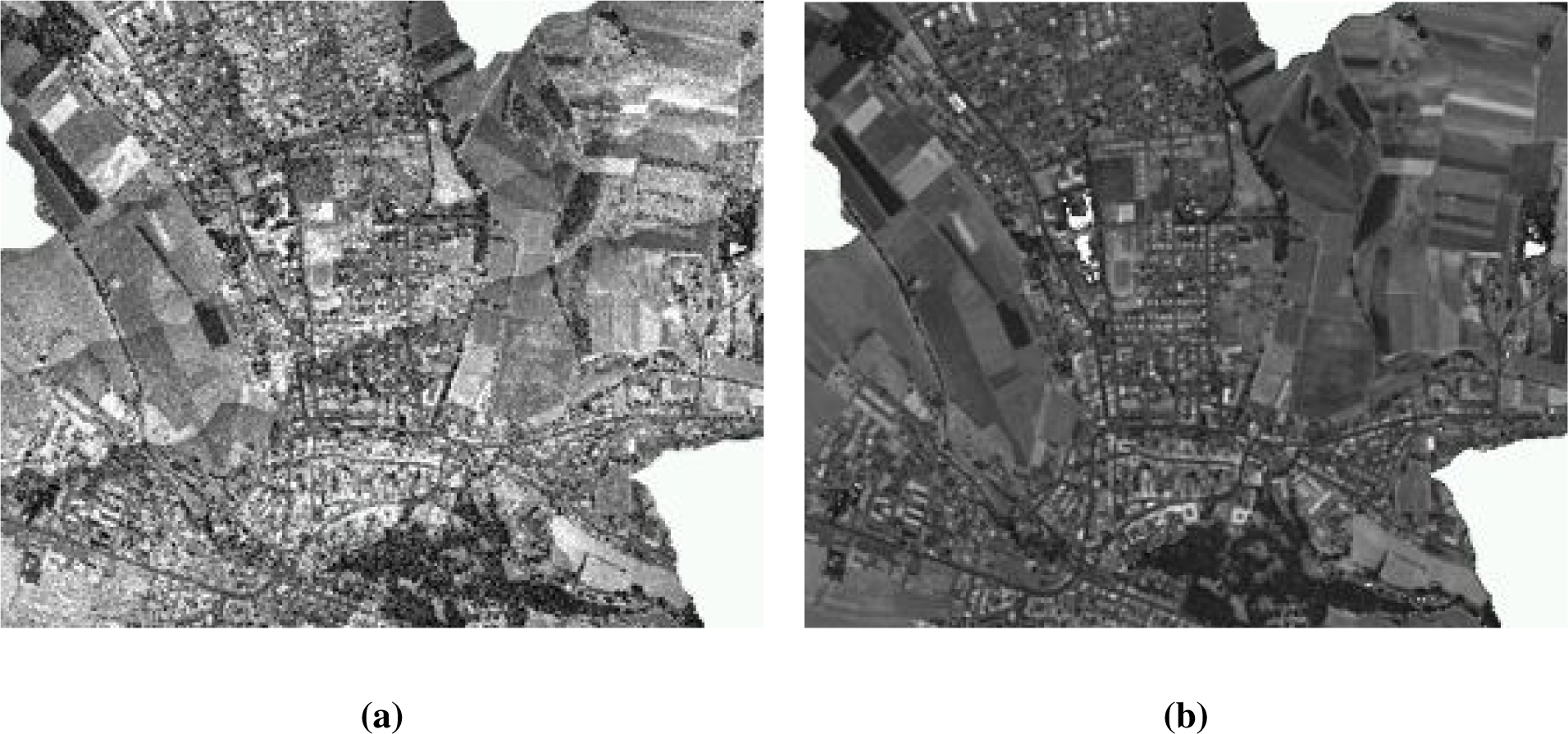
Features describing the local geometry are frequently used. Böhm and Pateraki [47] and Linsen et al. [48] use the surface normal vector and a distance to the neighboring points for point splatting. Point splatting is a method of rendering points with small surfaces, encoding the local distribution of points (e.g., oriented disks). The normal vector is estimated by fitting a plane that minimizes the Euclidean distance of the neighboring points to the plane. Abed et al. [49], in contrast, compute the normal vector based on a triangular mesh of the acquired point cloud, which requires meshing the data first. Normal vectors of the point clouds shown in Figure 1 are presented for a profile in Figure 2. Bae et al. [50] use, beyond the normal vector, also curvature and the variance of curvature for edge detection and segmentation of the point cloud. Zeming and Bingwei [51] also use the curvature feature, but for finding distinct points. The normal vector is a feature invariant to a shift of the coordinate system. Curvature, being a surface intrinsic description, is additionally invariant to rotation. Frome et al. [52] suggest using more complex shape descriptors for point cloud analysis, e.g., spin images [53], which are—in a tangent plane aligned coordinate system—histograms of a normalized point count of “horizontal” and “vertical” distance (A technical report on 3D shape descriptors is provided in Zhang et al. [54]). Their aim is to recognize objects in the point cloud. A similar approach is given in Steder et al. [55]. Ho and Gibbins [56] suggested to compute such features through the scale space, i.e., for neighborhoods of a different size. All these features can be interpreted geometrically. Monnier et al. [46] present a method based on entropy for optimal neighborhood selection using the scale space geometric features. Belongie et al. [57] propose the shape context, which differs, as it is a global description of the entire point cloud from the perspective of each single point.
Statistical features from the local neighborhood are described, e.g., in Yu et al. [58] using descriptors of the vertical point distribution, which are then used for predicting object properties. In the same category, Wang and Yuan [59] introduce density- and curvature-based features computed from the k (in their case, 15) nearest neighbors. The density-based feature is the average distance to the k nearest neighbors, and the curvature-based feature is the sum of the angles between the normal vector of the point and each of its neighboring point’s normal vector. Lalonde et al. [60] use the principal components of the point cloud in the neighborhood for classifying terrain for navigation purposes, more specifically, measures of linearity, “volumetricness” and “surfaceness” [61]. In Gressin et al. [62], statistical features are used for improving the relative orientation between point clouds using Iterative Closest Point (ICP). Next to the moments of the distributions of the coordinates in a neighborhood, Gibbins and Swierkowski [63] suggested additionally using moments invariant to rotation and the scale of the points and Zernike moments for point cloud classification. In some cases, these statistical features can also correspond to an object property, which has no geometric meaning, but still describes a perceptible quality. A further example is the echo ratio [9], which describes the permeability of a surface.
The contribution of specific features for urban classification was studied in Mallet et al. [64]. They grouped attributes into height features, eigenvalue features, local plane features, echo-based features and full waveform features. The last two groups are specific to laser scanning.
The features described above are either measured or computed from local neighborhoods. The measurement process itself also has an impact on the point itself, especially on the quality of its coordinates and feature values. Positional accuracies for each individual point can be derived in different ways. The empirical precisions of the measuring device, the measurement configuration and error propagation allow for estimating (a priori) accuracy. An internal or relative accuracy measure can be derived from over-determined measurement configuration, like multi-ray intersection (image matching) or overlapping data acquisitions (aerial and terrestrial laser scanning), etc. The computation of absolute accuracy, however, requires external reference data (of higher precision than the expected measurement accuracy) and rigorous measurement models in general [65]. The precision, or, more generally speaking, the quality, of the coordinates and attributes can therefore be considered as features of each point, as well.
3. Review of Data Structures and Neighborhoods
As billions of points may form a cloud, sophisticated organization is a requirement for efficient processing. Defining and finding the neighbors of a point is often performed on each point, thus “billions of times”. An overview on neighborhoods for point clouds is given in Filin and Pfeifer [66], complemented by a review of the varieties of neighborhoods, as suggested in the literature below. Next, data structures for large point clouds are discussed, as well as models for organizing attribute and geometric information.
3.1. Neighborhoods
A neighborhood of a point, Pi is a subset of the point cloud. Note that Pi does not need to be an element of the point cloud, but may also be a virtual point, and its nearest measurements are sought. Points are either considered neighbors if their distance to Pi is below a certain threshold or if they belong to the k closest points relative to Pi. The set of k closest points is not necessarily unique. In either case of the neighborhood, the distance must be measured. Distance can be measured in 2D, typically, the xy-plane, which makes sense for point clouds covering large areas and exhibiting a larger extent in xy than in z. Furthermore, for the analysis of the vertical structure, an analysis may meaningfully be confined to the 2D planimetric neighborhood. Otherwise, distances are measured in 3D.
The distance measure can be Euclidean, representing vertical cylinders and spheres to carve out the neighborhood in 2D and 3D, respectively. With anisotropic data distribution, these shapes may be affinely transformed, e.g., with a different z-scale than in xy. Alternatively, the Manhattan metric can be used, corresponding to coordinate differences. Within this description, also the cylindrical neighborhood is embedded, which measures radially in xy and absolute differences in z. The thresholds for horizontal and vertical distance (or planimetric and altimetric distance) must not be the same, which corresponds to a different scale in z.
Not all of the above neighborhoods are symmetric. Symmetry means for a neighborhood that points are mutually neighbors under a constant neighborhood definition. The maximum distance-based neighborhoods provide symmetry, whereas the k nearest neighborhoods do not. Other, nonsymmetric neighborhoods are the slope adaptive neighborhood [66] and the barycentric neighborhood [67]. The above neighborhood definitions can also be applied to quadrants or octants individually in order to provide a more symmetric distribution of the points around Pi. Furthermore, different neighborhood definitions can be applied together to further restrict the neighbors. An example is selecting in 2D in each quadrant the k nearest neighbors if they are below a maximum distance, r.
A triangulation or tetrahedronization can also be used to define a neighborhood [68,69]. This induces generations of neighborhoods, where the generation is the smallest number of edges that need to be traversed to reach a neighbor from Pi. This neighborhood requires the point Pi to be part of the triangulation and, therefore, typically of the entire point set.
The neighborhood size for computing features based on local neighborhood is often empirically chosen. The optimal neighborhood size depends on factors like point density, local curvature and noise levels [70]. Nothegger and Dorninger [71] propose a method for optimal neighborhood size for normal estimation and surface curvature analysis using the eigenvalues of the local structure tensor. Similarly, Demantké et al. [72] present a method based on entropy features of the local structure tensor for optimal radius selection, aiming at classifying local geometry into linear, planar and volumetric structures. A method for optimal neighborhood size determination for normal estimation is given in Mitra et al. [70].
3.2. Data Structures and Spatial Indices
The computation of neighborhoods within a point cloud takes significant effort independent of the neighborhood definition [73]. The neighborhoods defined in Section 3.1 can be translated into k nearest neighbor queries, fixed radius queries and range queries in 2D or 3D space. A naive search strategy answers those queries in O(n2) time, which is impractical for real world applications. Hence, it is necessary to use appropriate spatial data structures to speed up search queries. In this section, a review of different spatial indices is given. In the case of huge point clouds as obtained by current measurement technologies, the data clearly exceed the amount of available computer memory. Hence, the data need to be stored on secondary storage (like hard disk drives or solid state disks) and can be loaded into memory chunk-wise only. I/O (Input/Output) efficient data structures and processing strategies, as discussed in Section 3.3, are fundamental requirements to achieve effective data management.
Over the last three decades, a variety of different spatial indices have been developed, which subdivide the index space domain either in a regular or irregular manner [74]. Depending on geometry types (point, line, polygon, etc.), data distribution, query types and potential update operations, different indexing methods should be used. There is no optimal index for all situations. In the following, the most common indexing methods and their properties are described.
The k-d tree [75] is a very fast indexing method for nearest neighbor queries, but does not support line data. Additionally, the k-d tree rapidly gets unbalanced in the case of update operations (insertion or deletion of points). Quad- (2D index) and octree (3D index) structures are well suited for update operations and support point and polygonal data. However, they cannot compete with k-d trees in terms of speed when performing nearest neighbor queries [76]. As shown in [77], however, the specific implementation of the data structure (octree and k-d tree) also influences the speed of nearest neighbor and constant radius queries. Quad- and octrees are often used for visualization, since they can be easily adapted to support level-of-detail (LoD) structures. Such LoD information is required to realize efficient out-of-core rendering techniques [78].
Whereas quad- and octrees are limited in adapting to inhomogeneous data distributions, R-trees group nearby objects using minimum bounding rectangle or boxes in the next higher level of the tree. The key difficulty of R-trees is to build balanced trees and to minimize both the coverage and overlap of node bounding hyperboxes. However, R-trees tend to outperform quad- or octrees, e.g., [79,80], since it is possible to build balanced trees even in inhomogeneous data distributions. Heavy update activity can lead to unbalanced trees (or, at least, a lot of effort is needed to keep the tree balanced), which may outweigh the aforementioned advantage.
In certain situations, even linear structures, such as a simple tiling space partition [81] or lexicographically sorting by point coordinates [32], may be satisfactory.
3.3. Data Structures and Spatial Processing Concepts
The extraction of point features based on neighborhood information for an entire point cloud requires, next to appropriate spatial indices, also effective processing strategies. The precise adjustment of used spatial indices and processing schemas to the characteristics and distribution of the point data is necessary to achieve optimal performance.
The I/O (input/output) performance of secondary storage is often the limiting factor for such data-intense tasks. Hence, algorithms and their I/O complexity are reviewed in the following. Read (OI/O(r)) and write (OI/O(w)) operations are differentiated between, if possible (OI/O(rw), otherwise), since secondary storage, especially solid state disks (SSD), may show significant differences between read and write performance [82].
Isenburg et al. [83] proposed the concept of streaming algorithms to process huge point clouds. Their implementation of a streaming Delaunay triangulation utilizes the data in their natural order (i.e., the measurement sequence). While reading the point data, the algorithm makes use of a prior-built point count tree, allowing one to detect local regions that have been fully read. Those regions can then be further processed and eventually dropped from memory. Hence, only small parts of the point cloud are kept in memory at any one time, assuming that the input point data are somehow spatially sorted. This assumption holds for all standard point capturing methods or spatially pre-sorted (e.g., tiled) data. The advantage of omitting a pre-sorting step (e.g., explicitly building up a serialized data structure) does not come without disadvantages. First, the results are obtained in a “random” order and, therefore, usually require a post-processing sorting step. Additionally, the decision of when a local region can be processed depends on the computation method of the sought-after feature, causing a strong interdependence of different parts of the overall processing chain. The I/O complexity follows as OI/O(2 r(n) + sortpost).
A different concept using the natural acquisition topology of LiDAR data was proposed by David et al. [84] storing scan lines as pixel lines within multi-layer raster files. Assuming a regular scanning pattern, the multi-layer raster file provides an approximate spatial index onto the data, which can be satisfactory for strip-wise processing. This concept is implemented in the FullAnalyze project ( http://fullanalyze.sourceforge.net/).
A more generic way of efficient spatial access is either building up an independent spatial index containing references to the data only or directly inserting data into the spatial index itself. Both options have advantages and disadvantages, depending on the processing task to be fulfilled. Separate spatial index structures are usually much smaller than the point data itself, e.g., [85]. Hence, duplicating huge amounts of point data can be avoided in the case of appropriate source file formats (binary formats with random access). On the other hand, spatially sorted data usually lead to better performance in the case of multiple processing steps (since the processing order is usually better matched by the data order) and allow for implementing flexible and dynamic attribute schemas efficiently.
Persistent forms of spatial indices need to split the indexing domain only to a certain level to be I/O efficient (referred to as the first level index in the following). Leaf nodes (lowest level index nodes; end of branches), therefore, contain a substantial number of point data (e.g., >10,000) often described as bucket-sized [86]. On secondary storage, it is more efficient to read large blocks in sequence (sequential reads) than less information from different file locations (random reads) [87]. In the situation where such a coarse index does not provide satisfactory spatial performance, it is possible to temporarily extend the index on-the-fly. It is also possible to use a different index (secondary level index) that provides optimal performance for processing task to be carried out, such as, e.g., 3D nearest neighbor queries or real-time visualization [88].
Otepka et al. [89] proposed a tiling index as a first level index and k-d trees for each tile as a secondary index, which are built on-the-fly. Depending on the search queries, the k-d trees are built in two or three dimensions. Such a concept is appropriate for homogeneously distributed points over the ground plane domain, as is the case for airborne laser scanning and dense image matching. For situations with strongly varying point density (e.g., point clouds from terrestrial laser scanning), hierarchic structures, like quadtrees and R-trees, are more appropriate as the first level index. Whereas hierarchic structures can be usually built in OI/O(r(n) + rw(n log n)) time, a tiling structure requires only linear time (OI/O(r(n) + w(n))).
Applying spatial indices, it is straightforward to process huge datasets in appropriate chunks. To avoid processing artifacts at the chunk borders, an appropriate overlap from incident chunks is usually taken into consideration. To be I/O efficient and to optimize the overall performance, caching of loaded leafs is needed [90].
Tiled raster formats, such as tiled GeoTIFF (Georeferenced Tagged Image File Format), are commonly used for describing regular feature models (e.g., digital terrain models). For deriving such models, the tiles of the output format are usually used as processing chunk. On the other hand, extraction of features (e.g., local plane estimation, vertical point distribution, etc.) that are stored along each point can be efficiently performed based on the native spatial index structure in general. Sankaranarayanan et al. [73] described an optimized algorithm determining nearest neighbors for all points starting from the index leafs of the arbitrary persistent index structures.
3.4. Management of Additional Attributes
The methods described in this section so far were confined to the geometry, i.e., the coordinates. Here, concentration is put on the persistent storage of attributes. A very flexible scheme for handling the additional features can be implemented by managing attributes in tables of standard databases or similar structures. From a technical point of view, the attribute tables should support operations, such as the dynamic appending and dropping of table columns, and offer a variety of different data types and null values. Null values are useful, e.g., for marking attributes that were not computed successfully or that do not exist for some points. Such a system was presented by Höfle et al. [91], who uses PostGIS (Post-Geographic Information System) for storing the point information and Python commands to access and process the point cloud.
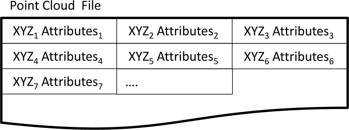
If point coordinates and attributes are stored in sequence, as shown in Figure 3, a direct link is given that secures fast access from points to their attributes. Such a structure, however, has a low degree of flexibility, since it requires a full re-write when appending or removing attributes. The problem can be reduced by reserving empty attribute storage in advance. The ASPRS (American Society of Photogrammetry and Remote Sensing) LiDAR data exchange format standard, LAS [92], implements such a concept. Beside standard attributes, like amplitude or time of measurement, as defined within the standard, it is also possible to append so-called “extra bytes” (of arbitrary length) to each point. Although this was possible from the first version of LAS (1.0), a generic way of describing the extra byte content was missing. This issue was tackled in LAS 1.4 (Extra Bytes Variable Length Record), making the format more powerful.
In case the attributes are managed in a separate structure, dynamic and more flexible concepts can be realized. Different attribute schemas can be represented by different attribute tables, as shown in Figure 4. Each point has a link to the data row in the corresponding attribute table [89]. The advantage of multiple attribute tables comes into play if only a subset of the data is appended with new attributes or datasets from different data sources are processed within a single project. This helps to minimize storage consumption.
In OPALS [93], the first level spatial index structure is reflected within the attribute tables. As shown in Figure 5, one attribute table per spatial index leaf is generated. For standard tasks (e.g., estimating a local plane in each point), the processing can be implemented based on the spatial index leafs. Due to the limited amount of data stored in each leaf, it is possible to fully load the corresponding points and their attributes into random access memory (RAM). There it is straightforward to set or append computed attributes efficiently. Once the leave is entirely processed, the attribute changes can be (incrementally or fully) written back to the attribute table. Due to the separated attribute table, this structure supports incremental updates on-the-fly and parallel processing, both on the basis of the spatial index leafs. The disadvantage of this concept is a certain managing overhead caused by multiple attribute tables and the extra effort needed to support efficient attribute-based queries (e.g., select all points with an amplitude above a certain threshold). Therefore, indices across the attribute tables are required.
4. Discussion and Proposals
4.1. Managing Point Cloud Data
The data in a point cloud can be separated into the coordinates and the features, respectively. Update operations can occur on both sets (appending new points) or on either of them by e.g., changing the coordinates of a point. Further examples are transformations to improve the georeferencing or the deletion of points due to blunder identification. Such global transformations result in a new point cloud, which requires rebuilding the spatial indices. Single points, like blunders, can be marked using (new) attributes, rather than stripping them from the dataset. Hence, efficient attribute updates are usually of a higher priority than adapting points and their coordinates.
As the variety of applications served by georeferenced point clouds is wide, the features used are very diverse, too. Therefore, flexible models were developed for multi-purpose point cloud processing, which can then exploit that some processing steps, e.g., classification, are the same. In this context, it is desirable to implement a method of data management that allows: (i) a free definition of attributes; (ii) appending and dropping attributes during processing; and (iii) a schema in which different points may have different attributes.
Models that provide this flexibility are, as shown above, either using a database or different attribute tables. Whereas existing databases and GIS provide reliable and flexible table schemas, there is a trade off between such a flexible model and high processing efficiency. This is tackled by the approaches above with attribute tables related to the first level spatial index. However, no comparative evaluation has been performed, yet. Schemes with one fixed list of attributes have advantages, due to their simplicity. Programs serving one specific purposes often use such a model (e.g., point cloud viewers (one example is FugroViewer, which has a constant list of attributes, www.fugroviewer.com)).
For feature computation, fast neighborhood queries are necessary. However, data structures should additionally support processing and/or visualizing the point could. As mentioned above, often, not the entire point cloud can be loaded into memory, and larger portions may have to be stored on secondary storage during the processing of extended areas. Thus, the spatial index for fast point access and persistent storage should be related to each other. This is reflected in the streaming approach of Isenburg et al. [83], as well as the two level spatial index, as used in OPALS [93].
4.2. Feature Categorization
Features of points can either be measured directly, obtained by processing the measurement, considering the measurements within the neighborhood, or computed in combination with other data sources. For satellite data products, a four tier specification is in use (see e.g., EPS/GGS/REQ/95327 Eumetsat document), with level 0 being the raw sensor readings, level 1, georeferenced and radiometrically calibrated values, level 2, retrieved environmental variables, and level 3, products obtained from the combination with other data. This advancement is illustrated in Figure 6. While the satellite product levels are not entirely suitable for georeferenced point clouds, the concept of advancing from the measurements to modeling is. Therefore, the proposed levels for point clouds are:
Level 0: the coordinates as generated and other measurements recorded by the sensor and directly related to the individual point;
Level 1: improved point coordinates from further georeferencing (if applicable) and the features obtained by the further processing of all measurements from one point, e.g., radiometrically calibrated quantities;
Level 2: features computed from the neighborhood of a point (either in the superior 3D space or in the sensor coordinate system); and
Level 3: features obtained by combining the above with other data sources.
Additionally, the review in Section 2.2 pointed out that the level 2 features are embedded in a scale space. The scale parameter is determined by the extent of the neighborhood used for computing the feature value. Furthermore, as part of the metadata, features should be accompanied with an estimation of their accuracy. This permits homogenization, i.e., the division of a feature value by its standard deviation, providing a unit-less number.
From Sections 2.1 and 2.2, the following level 0 features are identified. The point coordinates (x, y, z), which are independent of the measurement device: for image matching, this includes, additionally, the color of the points in the images, the forward intersection quality (number of rays, precision), the exposure times and the direction of the rays, which contain visibility information; for laser scanning, the additional features are the echo identifier (number of echo in the shot and total number of echoes per shot), the beam vector from sensor to point, the amplitude and echo width and the time of measurement.
Level 1 is composed of strict point features from calibrating and recombining the measurements associated with one point. The examples from above are the radiometrically calibrated reflectance, cross section and differential cross section parameters. Furthermore, intensity, hue and saturation are computed from the measurements of the individual point. In multispectral image analysis, different indices, e.g., NDVI (Normalized Difference Vegetation Index; see e.g., [94,95] for other indices.), are often used, falling into the same level. Note that object reflectivity using a model of Lambertian scatter does not fall into this group, because a normal vector needs to be estimated for its determination, which requires a calculation on a neighborhood.
The level 2 features are not restricted to one measurement, but encode the local behavior of the measured objects at a point of measurement. This can also be seen as a local model of the measured object. Thus, neighborhood definitions are required, including, especially, the size of the neighborhood. The measures of the local distribution can be moments, quantiles and their (robust) estimates, e.g., MAD (median of absolute deviations from the median; in the case of normal distributions, it is a robust estimator for the standard deviation if multiplied with the factor 1.4826 [96]). These moments can be computed for the z-coordinate, but also for the x- and y-coordinate or in a coordinate system adjusted to the local surface normal.
Furthermore, the distribution measures cannot only be determined for the point coordinates, but also for other features. Such a statistical feature is the measure of the local point density. Likewise, the SIFT-vector as a descriptor of the local image texture also falls in this category. While descriptors like SIFT can be used for any point (or pixel) in a set, it shall be noted that they are often applied to only a subset, namely, interest points (distinct points). Accordingly, Lowe [42] suggests an interest point detector and a descriptor for these key points. SIFT was also extended to a higher dimension, e.g., Flitton et al. [97] use it in 3D images created by computer tomography.
In level 2, also parameters of local models can become features of a point. They are obtained in two steps: first, a local model is computed from the points in the neighborhood (e.g., by least squares fitting a second order surface), and, as the second step, a parameter of this model is used as the feature of the point (e.g., the normal vector of the surface at the point of interest). These features are thus the tangent plane and normal vector, higher order surface descriptors (curvature), measures of the local model quality (e.g., RMSE (root mean square error) of the model), a measure of the deviation between the point and model, etc.
For level 2 features, it is of interest if they are invariant to shift, rotation and even scale. Invariance to shift and rotation applies to geometrical features that are based on the first and second derivative of a surface estimated from the neighboring points. This especially holds for planimetric shift and rotation, if a 2.5D surface model is computed (z = f(x, y)). If the surface model is computed independently of a parametrization, e.g., an orthogonal regression plane, it holds for all shifts and rotations. The SIFT descriptor is additionally invariant to scale, whereas other features are purposefully embedded in the scale space. An example for the scale space of feature values is given in Figure 7, in which the standard deviation of elevation is computed for the first echo points of a laser scanning point cloud. The radius increases from 2.0 m by factors of two to 16.0 m. The meadow in the foreground part of the image has constantly low dispersion, while the values with high dispersion change from the place of the crown intersection to the forest border. For the largest radius, also larger areas within the crown surface have a homogeneous dispersion, as the diameter is larger than a single tree.
Level 3 features are a general function of point features and a model at that point, e.g., the height of the point above the terrain, but also hyperspectral data given for a point obtained originally by laser scanning. Including a model from another source indicates the strong relation to a certain application. It is noted that class labels obtained from supervised classification also fall into this category. Because of the application dependency, the feature variety is much larger, and those features will not be discussed any further.
4.3. Processing Point Clouds with Features
The literature survey showed that the features used for processing georeferenced point clouds are very diverse. Still, it is possible to categorize those features. The suggested levels advance from raw data to more and more interpreted results.
Level 1 is a point cloud to be used for further processing. Arguments for keeping the point cloud are summarized in Axelsson [98] and Pfeifer et al. [99], specifically:
keeping the original resolution, which is otherwise lost in the generation of continuous models, due to interpolation;
keeping the 3D content of the data, including data void areas [37], which is otherwise lost in the generation of 2.5D models, due to the parameterization over xy; and
the impossibility to foresee which models or additional features need to be computed for a certain application in the future.
Level 1 data is typically data to be archived. Still, there is a distinction within level 1 features. Calibration advances the measurements from level 0, changing the unit, introducing a linear scale, etc. These values are derived using assumptions on the atmosphere and the measurement system. Those values mark a well-defined interface between data provision and data exploitation. However, radiometric calibration may only be performed if quantitative spectral evaluation is an envisaged application, but not otherwise. In that case, level 0 data would be archived, and the possibility for further calibration may be lost. In applications like visual interpretation of the point cloud, this is also not necessary.
Recombination of level 1 features of a single point does not increase the level. However, NDVI, as one example, can always be computed anew and does not necessarily need archiving. In satellite data product descriptions, intermediate levels were introduced (level 1a, 1b, etc.) to mark such differences. This is not suggested here.
In level 2, it is possible to distinguish between features that have a geometric interpretation, e.g., the normal vector, and others that describe the local distribution of points or other features. In level 2, neighborhood is introduced, which inherently assumes a certain continuity of the objects measured. Furthermore, for the geometrical features computed at level 2 to be meaningful, it must be assumed that the sampling is sufficiently dense, so that the local model can be estimated reliably.
In classification or segmentation tasks, level 0 features are rarely used successfully. Elevation alone can only be helpful in flat areas. If the raw amplitude or color is used, level 0 features require definition of training data to account for the dependency on mission parameters. Level 1 features, on the other hand, have a rather geo-physical meaning and, therefore, a meaningful unit, which can be related to object properties (e.g., absorption coefficients). This makes them also comparable between different data acquisition epochs, which does not hold for level 0 features. Still, deriving land cover classes from level 1 features is usually difficult, since the classes strongly overlap with respect to those features. As one example, house edges, as well as vegetation, exhibit multiple echoes in laser scanning point clouds. This is also similar to the overlap of spectral features of different land cover classes. One solution is using more spectral bands, i.e., choosing a sensor that provides more level 1 features in order to separate those classes.
However, alternatively to more level 1 features, the above problem of overlap between roof overhangs and vegetation in point clouds may also be alleviated by looking for linear structures (house edges) that are separated from area-wise occurrence (vegetation), which is equivalent to considering neighborhood, thus level 2 features. Instead of the linear structures for distinguishing between roof overhang and vegetation, a planarity measure can be used to separate those two. Planarity is expressed by the accuracy of plane fitting to the neighboring points of the investigated point; again, a level 2 feature.
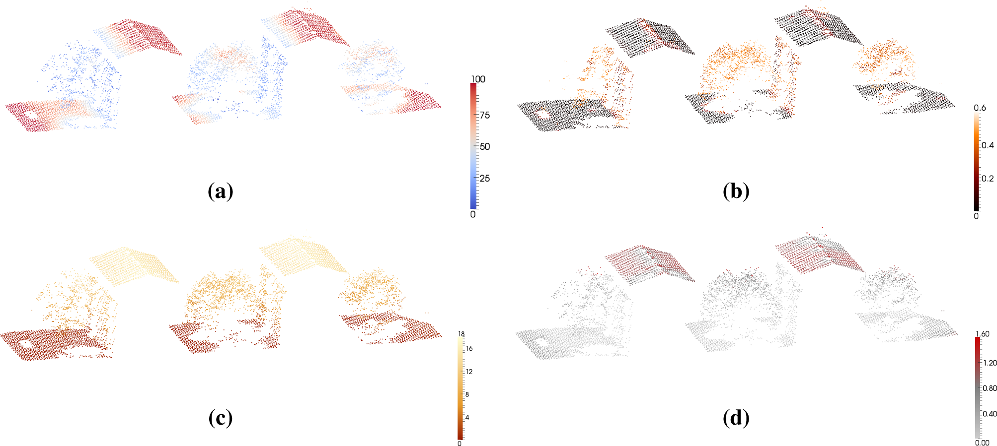
Examples illustrating the expressive power of level 2 features are given in Figure 8. The “echo ratio” [9] expresses whether, in a vertical view, the surface is solid or can be penetrated. Of course, this assumes that the line of sight for data acquisition is vertical, too. It is defined as the ratio of the number of points in a 3D neighborhood to the number of points in a 2D neighborhood, i.e., a neighborhood that is not restricted in z. The feature “sigma0” shows the plane fitting accuracy for the orthogonal regression plane in the 3D neighborhood. Not only the roofs, but also the points on a vertical wall are in flat neighborhoods, thus featuring a low sigma0 of a few centimeters only. Points in the vegetation, but also around the roof ridge and chimney, do not fit onto one plane, thus exhibiting a “noise” of up to 60 cm. The “normalized Z” is defined as the rank of the point (between zero and one) in the neighborhood multiplied with the range of z-values in the neighborhood. In the example with flat ground, it is equivalent to the height above ground. Finally, the positive openness shows the opening angle of a symmetric cone with the vertical axis and apex set to the analyzed point. The cone is opened as wide as possible so that it does not contain any other point. In Figure 8a, the influence of the radius (3 m) of the neighborhood becomes visible at the roof. In Figure 8c, the radius was set to 7 m, which means that always at least one ground point was included in the neighborhood.
These examples also illustrate that maintaining the point cloud as a source is superior to interpolating models, as the 3D content would be lost. Further examples highlighting this are presented in Höfle et al. [37], where the extraction of a water surface below overhanging vegetation is shown, or in Lindberg et al. [100], where extraction of subdominant trees is performed by point cloud clustering. Obviously, for terrestrially acquired point clouds, the 3D distribution of points is even more pronounced than for airborne acquired data. Thus, finding a suitable parameterization (plane) that preserves much of the characteristics is difficult, if not impossible (e.g., point clouds of forest scenes or of urban squares).
The investigation of Mallet et al. [64] indicated that a mixture of features from different levels performs better in classification. On the other hand, features of the same type, e.g., different distribution measures, do not increase classification accuracy.
Statistical values computed over all features within a point cloud become point cloud metadata. In a simple case, this includes the extents of an axis parallel bounding box of the points or the range of a certain attribute. Likewise, location or dispersion measures can be provided. However, also, a representative density of the data is an important characterization. Specifying a meaningful density is not independent of the application and defined very differently for terrestrial point clouds for forest inventory purposes or airborne point clouds for urban analysis. In the context of (airborne) area-wide acquisition, it is possible to define density as the number of points per square meter. Still, areas of overlapping data acquisition or characteristics of the measurement device need to be considered. In laser scanning, the number of emitted shots or the number of detected echoes can be specified per square-meter. In vegetation, the second one will be higher. Therefore, the definition of the term “density” is an integral part of the metadata description, not only the actual number itself.
5. Conclusions
This article gave a definition of a “georeferenced point cloud”, stressing especially the attributes of the points beyond their three coordinates in an Earth-fixed coordinate system. The features reviewed were considered first from a measurement technology point of view and, secondly, from their exploitation in point cloud processing, such as visualization, segmentation, classification and modeling. In the last case, thematic information is added to each individual point, which means that this class label becomes another feature (attribute) of that point. A categorization of the features into level 0 (raw measurements), level 1 (geometrically and radiometrically calibrated point clouds, enriched by recombination of the features of an individual point), level 2 (computed from the points in a neighborhood) and level 3 (computed by a combination with other models) was suggested. Classification and segmentation were not reviewed in this paper.
Keeping the native point cloud as opposed to the pure interpolation of surface models is advantageous for diverse applications, e.g., the classification of object space profits from keeping the 3D content, as well as the original distribution.
The structure for managing georeferenced point clouds is either based upon a regular subdivision of space, which has advantages for visualization, or based on data driven subdivisions, which is preferable for neighborhood queries. The latter one is important for the calculation of level 2 features.
Flexible models for defining and extending the features of the point cloud are essential for serving a great variety of applications. Nowadays, Geographic Information Systems (GISs), computer aided design (CAD) software or special extension packages provide tools to process point clouds. Their specific model, e.g., a standard list of features, can be more or less flexible as the ones presented within this paper.
Point clouds reach across disciplines, as their generation, processing, administration and presentation are of interest in geoinformation, computer vision, robotics and photogrammetry. Point clouds are a common denominator for processing laser scanning and photogrammetric data. Their difference lies only in the feature vector. Other differences, e.g., density, depend on mission parameters (e.g., flying height, sensor used), but also on the current state of technology (e.g., pixel pitch, pulse repetition rate). Figures 1 and 2 show such similarities, as well as differences. Hence, flexible point cloud processing is essential to serve this great variety.
Acknowledgments
Johannes Otepka, Sajid Ghuffar and Christoph Waldhauser were (partially) supported by the project “High Performance Computational Intelligence Methoden zur Auswertung von Airborne Laser Scanning Daten” of the Austrian Research Promotion Agency (FFG Bridge 832159). Sajid Ghuffar was additionally supported by the “Doctoral College on Computational Perception” at Vienna University of Technology. We acknowledge the support of Vermessung Schmid ZT GmbH, Inkustr. 1-7/3, 3400 Klosterneuburg, Austria, for their support of geodata. We would also like to thank the anonymous reviewers for their valuable input.
Conflicts of Interest
The authors declare no conflict of interest.
References
- Rieger, P. The Vienna laser scanning project. GEOconnex. Int. Mag. 2008, 7, 40–41. [Google Scholar]
- Mølhave, T.; Agarwal, P.; Arge, L.; Revsbæk, M. Scalable Algorithms for Large High-Resolution Terrain Data, Proceedings of the 1st International Conference and Exhibition on Computing for Geospatial Research & Application, Bethesda, MD, USA, 21–23 June 2010; p. 20.
- Li, Y.; Snavely, N.; Huttenlocher, D.; Fua, P. Worldwide Pose Estimation Using 3D Point Clouds, Proceedings of the International Conference on Computer Vision (ECCV), Florence, Italy, 7–13 October 2012.
- Altamimi, Z.; Collilieux, X.; Mtivier, L. ITRF2008: An improved solution of the international terrestrial reference frame. J. Geod. 2011, 85, 457–473. [Google Scholar]
- Nebiker, S.; Bleisch, S.; Christen, M. Rich point clouds in virtual globes—A new paradigm in city modeling? Comput. Environ. Urban Syst. 2010, 34, 508–517. [Google Scholar]
- Várady, T.; Martin, R.R.; Cox, J. Reverse engineering of geometric models—An introduction. Comput. Aided Des. 1997, 29, 255–268. [Google Scholar]
- Gorges, N.; Navarro, S.E.; Worn, H. Haptic Object Recognition Using Statistical Point Cloud Features, In Proceedings of the 15th International Conference on Advanced Robotics; pp. 15–20.
- Rutzinger, M.; Höfle, B.; Hollaus, M.; Pfeifer, N. Object-based point cloud analysis of full-waveform airborne laser scanning data for urban vegetation classification. Sensors 2008, 8, 4505–4528. [Google Scholar]
- Höfle, B.; Hollaus, M.; Hagenauer, J. Urban vegetation detection using radiometrically calibrated small-footprint full-waveform airborne LiDAR data. ISPRS J. Photogramm. Remote Sens. 2012, 67, 134–147. [Google Scholar]
- Crosby, C.J.; Arrowsmith, J.R.; Nandigam, V.; Baru, C. Online Access and Processing of Lidar Topography Data. In Geoinformatics; Cambridge University Press: Cambridge, UK, 2011; Chapter 16; pp. 251–256. [Google Scholar]
- Measures, R. Laser remote sensing: Present status and future prospects. Proc. SPIE 1997, 3059. [Google Scholar] [CrossRef]
- Yastikli, N.; Jacobsen, K. Direct sensor orientation for large scale mapping—Potential, problems, solutions. Photogramm. Rec. 2005, 20, 274–284. [Google Scholar]
- Höfle, B.; Pfeifer, N. Correction of laser scanning intensity data: Data and model-driven approaches. ISPRS J. Photogramm. Remote Sens. 2007, 62, 415–433. [Google Scholar]
- Kaasalainen, S.; Ahokas, E.; Hyyppa, J.; Suomalainen, J. Study of surface brightness from backscattered laser intensity: Calibration of laser data. IEEE Geosci. Remote Sens. Lett. 2005, 2, 255–259. [Google Scholar]
- Wagner, W.; Ullrich, A.; Ducic, V.; Melzer, T.; Studnicka, N. Gaussian decomposition and calibration of a novel small-footprint full-waveform digitising airborne laser scanner. ISPRS J. Photogramm. Remote Sens. 2006, 60, 100–112. [Google Scholar]
- Mallet, C.; Lafarge, F.; Roux, M.; Soergel, U.; Bretar, F.; Heipke, C. A marked point process for modeling lidar waveforms. IEEE Trans. Image Process. 2010, 19, 3204–3221. [Google Scholar]
- Chauve, A.; Mallet, C.; Bretar, F.; Durrieu, S.; Deseilligny, M.; Puech, W. Processing Full-Waveform Lidar Data: Modelling Raw Signals, Proceedings of the International Archives of Photogrammetry and Remote Sensing, Espoo, Finland, 12–14 September 2007.
- Roncat, A.; Bergauer, G.; Pfeifer, N. B-spline deconvolution for differential target cross-section determination in full-waveform laser scanner data. ISPRS J. Photogramm. Remote Sens. 2011, 66, 418–428. [Google Scholar]
- Duong, H.V. Processing and Application of ICESat Large Footprint Full Waveform Laser Range Data. Ph.D. Thesis, Delft University of Technology, Delft, The Netherlands, 2010. [Google Scholar]
- Lillesand, T.M.; Kiefer, R.W.; Chipman, J.W. Remote Sensing and Image Interpretation, 6 ed.; John Wiley & Sons Ltd: Hoboken, NJ, USA, 2007. [Google Scholar]
- Honkavaara, E.; Arbiol, R.; Markelin, L.; Martinez, L.; Cramer, M.; Bovet, S.; Chandelier, L.; Ilves, R.; Klonus, S.; Marshal, P.; et al. Digital airborne photogrammetry—A new tool for quantitative remote sensing?—A state-of-the-art review on radiometric aspects of digital photogrammetric images. Remote Sens. 2009, 1, 577–605. [Google Scholar]
- Schaepman-Strub, G.; Schaepman, M.; Painter, T.; Dangel, S.; Martonchik, J. Reflectance quantities in optical remote sensing—Definitions and case studies. Remote Sens. Environ. 2006, 103, 27–42. [Google Scholar]
- Hirschmüller, H. Stereo processing by semi-global matching and mutual information. IEEE Trans. Pattern Anal. Mach. Intell. 2008, 30, 328–341. [Google Scholar]
- Kraus, K. 8.1.2.1. Georeferencing. In Photogrammetry—Geometry from Images and Laser Scans, 2 ed.; De Gruyter: Berlin, Germany, 2007; pp. 459–475. [Google Scholar]
- Cramer, M.; Stallmann, D.; Haala, N. Direct Georeferencing Using GPS/Inertial Exterior Orientations for Photogrammetric Applications, Proceedings of the International Archives of Photogrammetry and Remote Sensing, Amsterdam, The Netherlands, 16–22 July 2000; 33, pp. 198–205.
- Heipke, C.; Jacobsen, K.; Wegmann, H.; Andersen, Ø.; Nilsen, B. Integrated Sensor Orientation—An OEEPE Test, In Proceedings of the International Archives of Photogrammetry and Remote Sensing, Amsterdam, The Netherlands, 16–22 July 2000; 33, pp. 373–380.
- Heipke, C.; Jacobsen, K.; Wegmann, H. Analysis of the results of the OEEPE test “Integrated Sensor Orientation”. OEEPE Off. Publ. 2002, 43, 31–49. [Google Scholar]
- Leberl, F. Imaging radar applications to mapping and charting. Photogrammetria 1976, 32, 75–100. [Google Scholar]
- Toutin, T.; Gray, L. State-of-the-art of elevation extraction from satellite SAR data. ISPRS J. Photogramm. Remote Sens. 2000, 55, 13–33. [Google Scholar]
- Zhu, X.; Bamler, R. Very high resolution spaceborne SAR tomography in urban environment. IEEE Trans. Geosci. Remote Sens. 2010, 48, 4296–4308. [Google Scholar]
- Amiri-Simkooei, A.; Snellen, M.; Simons, D.G. Riverbed sediment classification using multi-beam echo-sounder backscatter data. J. Acoust. Soc. Am. 2009, 126. [Google Scholar] [CrossRef]
- Arge, L.; Larsen, K.G.; Mølhave, T.; van Walderveen, F. Cleaning Massive Sonar Point Clouds, Proceedings of 18th ACM SIGSPATIAL International Conference on Advances in Geographic Information Systems (GIS’10), San Jose, CA, USA, 2–5 November 2010.
- Kohoutek, T.; Nitsche, M.; Eisenbeiss, H. Geo-referenced mapping using an airborne 3D time-of-flight camera. Arch. Photogramm. Remote Sens. Spatial Inf. Sci. 2011. [Google Scholar] [CrossRef]
- Wand, M.; Berner, A.; Bokeloh, M.; Jenke, P.; Fleck, A.; Hoffmann, M.; Maier, B.; Staneker, D.; Schilling, A.; Seidel, H.P. Processing and interactive editing of huge point clouds from 3D scanners. Comput. Graph. 2008, 32, 204–220. [Google Scholar]
- Lichti, D. Spectral filtering and classification of terrestrial laser scanner point clouds. Photogramm. Rec. 2005, 20, 218–240. [Google Scholar]
- Briese, C.; Pfennigbauer, M.; Lehner, H.; Ullrich, A.; Wagner, W.; Pfeifer, N. Radiometric Calibration of Multi-Wavelength Airborne Laser Scanning Data, Proceedings of the ISPRS Annals of the Photogrammetry, Remote Sensing and Spatial Information Sciences (ISPRS Annals); I-7, pp. 335–340.
- Höfle, B.; Vetter, M.; Pfeifer, N.; Mandlburger, G.; Stötter, J. Water surface mapping from airborne laser scanning using signal intensity and elevation data. Earth Surface Process. Landf. 2009, 34, 1635–1649. [Google Scholar]
- Hollaus, M.; Mücke, W.; Höfle, B.; Dorigo, W.; Pfeifer, N.; Wagner, W.; Bauerhansl, C.; Regner, B. Tree Species Classification Based on Full-Waveform Airborne Laser Scanning Data, Proceedings of the SILVILASER 2009, Denver, CO, USA, 14–16 October 2009.
- Heinzel, J.; Koch, B. Exploring full-waveform LiDAR parameters for tree species classification. Int. J. Appl. Earth Obs. Geoinf. 2011, 13, 152–160. [Google Scholar]
- Alexander, C.; Tansey, K.; Kaduk, J.; Holland, D.; Tate, N. Backscatter coefficient as an attribute for the classification of full-waveform airborne laser scanning data in urban areas. ISPRS J. Photogramm. Remote Sens. 2010, 65, 423–432. [Google Scholar]
- Neuenschwander, A.; Magruder, L.; Tyler, M. Landcover classification of small-footprint, full-waveform lidar data. J. Appl. Remote Sens. 2009, 3. [Google Scholar] [CrossRef]
- Lowe, D.G. Distinctive image features from scale-invariant keypoints. Int. J. Comput. Vis. 2004, 60, 91–110. [Google Scholar]
- Clode, S.; Rottensteiner, F. Classification of Trees and Powerlines from Medium Resolution Airborne Laserscanner Data in Urban Environments, Proceedings of the APRS Workshop on Digital Image Computing (WDIC), Brisbane, Australia, 21 February 2005.
- Brzank, A.; Heipke, C.; Goepfert, J.; Soergel, U. Aspects of generating precise digital terrain models in the Wadden Sea from lidar-water classification and structure line extraction. ISPRS J. Photogramm. Remote Sens. 2008, 63, 510–528. [Google Scholar]
- Hammoudi, K.; Dornaika, F.; Soheilian, B.; Vallet, B.; McDonald, J.; Paparoditis, N. Recovering occlusion-free textured 3D maps of urban facades by a synergistic use of terrestrial images, 3D point clouds and area-based information. Procedia Eng. 2012, 41, 971–980. [Google Scholar]
- Monnier, F.; Vallet, B.; Soheilian, B. Trees Detection from Laser Point Clouds Acquired in Dense Urban Areas by a Mobile Mapping System, Proceedings of the ISPRS Annals of the Photogrammetry, Remote Sensing and Spatial Information Sciences (ISPRS Annals), Melbourne, Australia, 25 August–1 September 2012; I-3, pp. 245–250.
- Böhm, J.; Pateraki, M. From point samples to surfaces-on meshing and alternatives. Int. Arch. Photogramm. Remote Sens. 2007, XXXVI/V, 50–55. [Google Scholar]
- Linsen, L.; Müller, K.; Rosenthal, P. Splat-Based Ray Tracing of Point Clouds, Proceedings of the 15th International Conference in Central Europe on Computer Graphics, Visualization and Computer Vision 2007 (WSCG’2007), Bory, Czech Republic, 29 January–1 February 2007.
- Abed, F.; Mills, J.P.; Miller, P.E. Echo amplitude normalization of full-waveform airborne laser scanning data based on robust incidence angle estimation. IEEE Trans. Geosci. Remote Sens. 2012, 50, 2910–2918. [Google Scholar]
- Bae, K.; Belton, D.; Lichti, D.D. Pre-processing procedures for raw point clouds from terrestrial laser scanners. J. Spat. Sci. 2007, 52, 65–74. [Google Scholar]
- Zeming, L.; Bingwei, H. A Curvature-Based Automatic Registration Algorithm for the Scattered Points, Proceedings of the 2011 Third International Conference on Measuring Technology and Mechatronics Automation (ICMTMA), Shanghai, China, 6–7 January 2011; 1, pp. 28–31.
- Frome, A.; Huber, D.; Kolluri, R.; Bulow, T.; Malik, J. Recognizing Objects in Range Data Using Regional Point Descriptors, Proceedings of the European Conference on Computer Vision (ECCV), Prague, Czech Republic, 11–14 May 2004.
- Johnson, A.; Hebert, M. Using spin images for efficient object recognition in cluttered 3D scenes. IEEE Trans. Pattern Anal. Mach. Intell. 1999, 21, 433–449. [Google Scholar]
- Zhang, L.; da Fonseca, M.; Ferreira, A. Survey on 3D Shape Descriptors; Technical Report, DecorAR (FCT POSC/EIA/59938/2004); Fundação para a Cincia e a Tecnologia: Lisboa, Portugal, 2007. [Google Scholar]
- Steder, B.; Rusu, R.; Konolige, K.; Burgard, W. Point Feature Extraction on 3D Range Scans Taking into Account Object Boundaries 2601–2608.
- Ho, H.; Gibbins, D. Curvature-based approach for multi-scale feature extraction from 3D meshes and unstructured point clouds. Comput. Vis. IET 2009, 3, 201–212. [Google Scholar]
- Belongie, S.; Malik, J.; Puzicha, J. Shape matching and object recognition using shape contexts. IEEE Trans. Pattern Anal. Mach. Intell. 2002, 24, 509–522. [Google Scholar]
- Yu, X.; Hyyppä, J.; Vastaranta, M.; Holopainen, M.; Viitala, R. Predicting individual tree attributes from airborne laser point clouds based on the random forests technique. ISPRS J. Photogramm. Remote Sens. 2011, 66, 28–37. [Google Scholar]
- Wang, L.; Yuan, B. Curvature and Density Based Feature Point Detection for Point Cloud Data, Proceedings of the IET 3rd International Conference on Wireless, Mobile and Multimedia Networks (ICWMMN 2010), Beijing, China, 26–29 September 2010.
- Lalonde, J.F.; Vandapel, N.; Huber, D.; Hebert, M. Natural terrain classification using three-dimensional ladar data for ground robot mobility. J. Field Robot. 2006, 23, 839–861. [Google Scholar]
- Medioni, G.; Lee, M.S.; Tang, C.K. A Computational Framework for Segmentation and Grouping; Elsevier: Amsterdam, The Netherlands, 2000. [Google Scholar]
- Gressin, A.; Mallet, C.; David, N. Improving 3D Lidar Point Cloud Registration Using Optimal Neighborhood Knowledge, Proceedings of ISPRS Annals of the Photogrammetry, Remote Sensing and Spatial Information Sciences, Melbourne, Australia, 5 August–1 September 2012; pp. 111–116.
- Gibbins, D.; Swierkowski, L. A Comparison of Terrain Classification Using Local Feature Measurements of 3-Dimensional Colour Point-Cloud Data, Proceedings of the 24th International Conference on Image and Vision Computing New Zealand (IVCNZ ’09), Palmerston North, New Zealand, 23–25 November 2009; pp. 293–298.
- Mallet, C.; Bretar, F.; Roux, M.; Soergel, U.; Heipke, C. Relevance assessment of full-waveform lidar data for urban area classification. ISPRS J. Photogramm. Remote Sens. 2011, 66, S71–S84. [Google Scholar]
- Ressl, C.; Kager, H.; Mandlburger, G. Quality checking of ALS projects using statistics of strip differences. Int. Arch. Photogramm. Remote Sens. Spatial Inf. Sci. 2008, XXXVII/3B, 253–260. [Google Scholar]
- Filin, S.; Pfeifer, N. Neighborhood systems for airborne laser data. Photogramm. Eng. Remote Sens. 2005, 71, 743–755. [Google Scholar]
- Chaudhuri, B. A new definition of neighborhood of a point in multi-dimensional space. Pattern Recognit. Lett. 1996, 17, 11–17. [Google Scholar]
- Gorte, B. Segmentation of TIN-structured surface models. Int. Arch. Photogramm. Remote Sens. Spatial Inf. Sci. 2002, 34, 465–469. [Google Scholar]
- Maas, H.G.; Vosselman, G. Two algorithms for extracting building models from raw laser altimetry data. ISPRS J. Photogramm. Remote Sens. 1999, 54, 153–163. [Google Scholar]
- Mitra, N.J.; Nguyen, A.; Guibas, L. Estimating surface normals in noisy point cloud data. Int. J. Comput. Geom. Appl. 2004, 14, 261–276. [Google Scholar]
- Nothegger, C.; Dorninger, P. 3D filtering of high-resolution terrestrial laser scanner point clouds for cultural heritage documentation. Photogramm. Fernerkund. Geoinf. 2009, 2009, 53–63. [Google Scholar]
- Demantké, J.; Mallet, C.; David, N.; Vallet, B. Dimensionality Based Scale Selection in 3D Lidar Point Clouds, Proceedings of ISPRS Workshop, Laser scanning 2011, Calgary, AB, Canada, 29–31 August 2011.
- Sankaranarayanan, J.; Samet, H.; Varshney, A. A fast all nearest neighbor algorithm for applications involving large point-clouds. Comput. Graph. 2007, 31, 157–174. [Google Scholar]
- Samet, H. The Design and Analysis of Spatial Data Structures; Addison Wesley: Reading, MA, USA, 1989. [Google Scholar]
- Bentley, J.L. Multidimensional binary search trees used for associative searching. Commun. ACM 1975, 18, 509–517. [Google Scholar]
- Zinßer, T.; Schmidt, J.; Niemann, H. Performance Analysis of Nearest Neighbor Algorithms for ICP Registration of 3-D Point Sets, Proceedings of the 8th International Fall Workshop of Vision, Modeling, and Visalization, Munich, Germany, 19–21 November 2003.
- Elseberg, J.; Magnenat, S.; Siegwart, R.; Nüchter, A. Comparison of nearest-neighbor-search strategies and implementations for efficient shape registration. J. Softw. Eng. Robots. 2012, 3, 2–12. [Google Scholar]
- Richter, R.; Döllner, J. Out-of-Core Real-Time Visualization of Massive 3D Point Clouds, Proceedings of the 7th International Conference on Computer Graphics, Virtual Reality, Visualisation and Interaction in Africa (AFRIGRAPH ’10), Franschoek, South Africa, 21–23 June 2010; ACM: New York, NY, USA, 2010; pp. 121–128.
- Kothuri, R.K.V.; Ravada, S.; Abugov, D. Quadtree and R-Tree Indexes in Oracle Spatial: A Comparison Using GIS Data, Proceedings of the 2002 ACM SIGMOD International Conference on Management of Data (SIGMOD ’02), 3–6 June 2002; ACM, 2002; pp. 546–557.
- Kim, Y.J.; Patel, J.M. Performance comparison of the R*-tree and the quadtree for kNN and distance join queries. IEEE Trans. Knowl. Data Eng. 2010, 22, 1014–1027. [Google Scholar]
- Mandlburger, G.; Otepka, J.; Karel, W.; Wagner, W.; Pfeifer, N. Orientation and Processing of Airborne Laser Scanning Data (Opals)—Concept and First Results of a Comprehensive ALS Software, Proceedings of the ISPRS Workshop Laserscanning ’09, Paris, France, 1–2 September 2009; pp. 55–60.
- Dirik, C.; Jacob, B. The Performance of PC Solid-State Disks (SSDs) as a Function of Bandwidth, Concurrency, Device Architecture, and System Organization, Proceedings of the 36th Annual International Symposium on Computer Architecture (ISCA ’09), 20–24 June 2009; ACM, 2009; pp. 279–289.
- Isenburg, M.; Liu, Y.; Shewchuk, J.; Snoeyink, J. Streaming Computation of Delaunay Triangulations, Proceedings of the SIGGRAPH’06, Boston, MA, USA, 30 July–3 August 2006; pp. 1049–1056.
- David, N.; Mallet, C.; Bretar, F. Library Concept and Design for Lidar Data Processing, Proceedings of the GEOgraphic Object Based Image Analysis (GEOBIA) Conference, Calgary, AB, Canada, 5–8 August 2008.
- Isenburg, M. LASindex—Spatial Indexing of LiDAR Data, 2013. Available online: http://rapidlasso.com/category/videos accessed on 18 October 2013.
- Guttman, A. R-Trees: A Dynamic Index Structure for Spatial Searching, Proceedings of the International Conference on Management of Data, Boston, MA, USA, 18–21 June 1984; pp. 47–57.
- Atkin, I. Getting the Hang of IOPS, an Introduction to Disk Performance; Technical Report; The University Of Oxford’s ICT Support Team: Oxford, UK, 2012. Available online: http://www.symantec.com/connect/articles/getting-hang-iops-v13 accessed on 18 October 2013.
- Wimmer, M.; Scheiblauer, C. Instant Points: Fast Rendering of Unprocessed Point Clouds, Proceedings of the 3rd Eurographics/IEEE VGTC Conference on Point-Based Graphics (SPBG’06), Boston, MA, USA, 29–30 July 2006; Eurographics Association: Aire-la-Ville, Switzerland, 2006; pp. 129–137.
- Otepka, J.; Mandlburger, G.; Karel, W. The OPALS Data Manager—Efficient Data Management for Processing Large Airborne Laser Scanning Projects, Proceedings of the ISPRS Annals of the Photogrammetry, Melbourne, Australia, 25 August–1 September, 2012; I-3, pp. 153–159.
- Kreylos, O.; Bawden, G.W.; Kellogg, L.H. Immersive Visualization and Analysis of LiDAR Data, Proceedings of the 4th International Symposium on Advances in Visual Computing (ISVC ’08), Las Vegas, NV, USA, 1–3 December 2008; Springer-Verlag: Berlin/Heidelberg, Germany, 2008; pp. 846–855.
- Höfle, B.; Rutzinger, M.; Geist, T.; Stötter, J. Using Airborne Laser Scanning Data in Urban Data Management—Set up of a Flexible Information System with Open Source Components, Proceedings of Urban Data Management Symposium (UDMS 2006), Aalborg, Denmark, 15–17 May 2006; pp. 7.11–7.23.
- ASPRS. LAS File Format Exchange Activities; Homepage of ASPRS LAS File Format, 2011. Available online: http://www.asprs.org/Committee-General/LASer-LAS-File-Format-Exchange-Activities.html accessed on 18 October 2013.
- OPALS. Orientation and Processing of Airborne Laser Scanning Data (Product Homepage). Department of Geodesy and Geoinformation—Research Groups Photogrammetry and Remote Sensing, 2013. Available online: http://geo.tuwien.ac.at/opals accessed on 18 October 2013.
- Bannari, A.; Morin, D.; Bonn, F.; Huete, A. A review of vegetation indices. Remote Sens. Rev. 1995, 13, 95–120. [Google Scholar]
- Stagakis, S.; González-Dugo, V.; Cid, P.; Guillén-Climent, M.; Zarco-Tejada, P. Monitoring water stress and fruit quality in an orange orchard under regulated deficit irrigation using narrow-band structural and physiological remote sensing indices. ISPRS J. Photogramm. Remote Sens. 2012, 71, 47–61. [Google Scholar]
- Maronna, R.; Martin, D.; Yohai, V. Robust Statistics: Theory and Methods; Wiley: Chichester, UK, 2006. [Google Scholar]
- Flitton, G.; Breckon, T.; Megherbi, N. A comparison of 3D interest point descriptors with application to airport baggage object detection in complex CT imagery. Pattern Recognit. 2013, 46, 2420–2436. [Google Scholar]
- Axelsson, P. Processing of laser scanner data—Algorithms and applications. ISPRS J. Photogramm. Remote Sens. 1999, 54, 138–147. [Google Scholar]
- Pfeifer, N.; Mandlburger, G.; Otepka, J.; Karel, W. OPALS—A framework for airborne laser scanning data analysis. Comput. Environ. Urban Syst. 2013. submitted. [Google Scholar]
- Lindberg, E.; Holmgren, J.; Olofsson, K.; Wallerman, J.; Olsson, H. Estimation of tree lists from airborne laser scanning using tree model clustering and k-MSN imputation. Remote Sens. 2013, 5, 1932–1955. [Google Scholar]

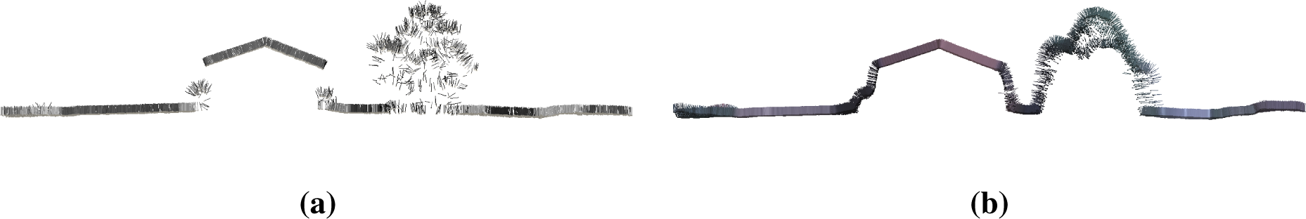


© 2013 by the authors; licensee MDPI, Basel, Switzerland This article is an open access article distributed under the terms and conditions of the Creative Commons Attribution license (http://creativecommons.org/licenses/by/3.0/).
Share and Cite
Otepka, J.; Ghuffar, S.; Waldhauser, C.; Hochreiter, R.; Pfeifer, N. Georeferenced Point Clouds: A Survey of Features and Point Cloud Management. ISPRS Int. J. Geo-Inf. 2013, 2, 1038-1065. https://doi.org/10.3390/ijgi2041038
Otepka J, Ghuffar S, Waldhauser C, Hochreiter R, Pfeifer N. Georeferenced Point Clouds: A Survey of Features and Point Cloud Management. ISPRS International Journal of Geo-Information. 2013; 2(4):1038-1065. https://doi.org/10.3390/ijgi2041038
Chicago/Turabian StyleOtepka, Johannes, Sajid Ghuffar, Christoph Waldhauser, Ronald Hochreiter, and Norbert Pfeifer. 2013. "Georeferenced Point Clouds: A Survey of Features and Point Cloud Management" ISPRS International Journal of Geo-Information 2, no. 4: 1038-1065. https://doi.org/10.3390/ijgi2041038
APA StyleOtepka, J., Ghuffar, S., Waldhauser, C., Hochreiter, R., & Pfeifer, N. (2013). Georeferenced Point Clouds: A Survey of Features and Point Cloud Management. ISPRS International Journal of Geo-Information, 2(4), 1038-1065. https://doi.org/10.3390/ijgi2041038